Optimal Planning of Dynamic Thermal Management for NANS (N-App N-Screen) Services †

Department of Computer Science and Engineering, Seoul National University, 1 Gwanak-Ro, Gwanak-Gu, Seoul 08826, Korea
*
Author to whom correspondence should be addressed.
†
This paper is an extended version of our paper published in Proceedings of the 13th International Symposium on Industrial Embedded Systems (SIES ’18), Graz, Austria, 6–8 June 2018.
Electronics 2018, 7(11), 311; https://doi.org/10.3390/electronics7110311
Submission received: 26 September 2018
/
Revised: 4 November 2018
/
Accepted: 5 November 2018
/
Published: 8 November 2018
(This article belongs to the Special Issue Challenges and Opportunities of IoT Deployments—Avoiding the Internet of Junk)
Abstract
:Existing multi-screening technologies have been limited to mirroring the current screen of the smartphone onto all the connected external display devices. In contrast, NANS (N-App N-Screen) technology is able to display different applications (N-App) on different multiple display devices (N-Screen) using only a smartphone. For such NANS services, this paper empirically shows that the thermal violation constraint is more critical than the battery life constraint. For preventing the thermal violation, the existing DTM (Dynamic Thermal Management) techniques cannot be used since they consider thermal violations as abnormal, and hence prevent them by severely throttling CPU frequencies resulting in serious QoS degradation. In NANS service scenarios it is normal to operate in high temperature ranges to continue services with acceptable QoS. Targeting such scenarios, we first propose a novel thermal prediction method specially designed for NANS services. Based on the novel thermal prediction method, we then propose a novel DTM technique called, “thermal planning” to provide sustainable NANS services with sufficiently high QoS without thermal violations.
1. Introduction
Thanks to the advance of recent display interface technologies such as wireless Miracast [1] or wired HDMI (High Definition Multimedia Interface) [2], users can connect their smartphones to external large display devices such as TVs and PC monitors. Through these display interfaces, Mirroring, i.e., a typical multi-screening technique, mirrors the current screen of the smartphone onto all the connected external display devices as shown in Figure 1a. Mirroring cannot meet the user’s needs for using the smartphone display and external displays for displaying multiple different applications. For example, it is not possible to show a mobile messenger on the smartphone display, a movie player on the TV display, and a web browser on the tablet display simultaneously.
To realize such multi-screening scenarios on smartphones, we developed NANS (N-App N-Screen) technology [3], which is now available as an open source project. NANS technology is implemented by improving Android mobile platform in such a way that multiple applications (N-App) are concurrently executed and rendered on a smartphone and their rendered images are transmitted to multiple desired displays (N-Screen) as shown in Figure 1b. The detailed description and video demonstrations of NANS technology can be found on our open source project [3]. Compared to using multiple separate devices, NANS technology has obvious advantages in terms of service continuity. With NANS technology, a user can display all the content of a smartphone, such as applications, movies, music, pictures, and personal data, on surrounding display devices without re-installing applications or copying content to those devices.
NANS technology has to overcome a big hurdle to become a commercially deployable solution. The rapid temperature increase caused by the enormous use of smartphone resources for executing and rendering multiple applications and transmitting their rendered images concurrently is problematic [4]. The rapid increase in temperature of hardware components quickly results in thermal violation that exceeds the thermal threshold limited by the chip manufacturer. The thermal violation of microprocessors is a well-known cause of increasing leakage current and lowering chip reliability [5].
To protect microprocessors from thermal violations, there have been many studies on thermal prediction-based DTM (Dynamic Thermal Management) [6,7,8,9,10,11,12,13,14,15,16] to predict the temperature and then to lower the resource usage if the predicted temperature is at risk of exceeding the thermal threshold. Since those studies consider rapid temperature increases as abnormal and rare cases, they use simple solutions despite the risk of thermal violations. For example, even a thermal prediction method with large errors above 10 °C is still acceptable since we can use it with enough thermal budget to pessimistically predict the thermal violation. The penalty by such a pessimistic thermal prediction is not that serious if a temperature increase close to the thermal threshold rarely happens. Also, based on such a pessimistic thermal prediction, rather simple solutions such as lowering the microprocessor’s frequency or shutting-down can be used in smartphones. If such cases happen rarely, it does not seriously harm the user’s quality of experience.
However, in NANS service scenarios, it is not abnormal but rather typical for smartphones to be operated at a high temperature range close to the thermal threshold. The above solutions, which treat temperature increases approaching the thermal threshold as abnormal cases, cannot be used directly [17]. For NANS services, firstly, we need a reliable thermal prediction method that works well even at high temperature ranges close to the thermal threshold. Secondly, we need a thermal management technique to carefully minimize the negative impact on the user experience, even at high temperature ranges. Considering these two points, in this paper, we propose a novel DTM especially designed for NANS services. The contributions of this paper are summarized as follows:
- Firstly, we propose a novel thermal prediction method especially designed for NANS services. For this, we extend the existing thermal model by identifying the major heat sources in NANS technology and considering the thermal interaction between these heat sources. Also, our proposed thermal prediction method additionally models our new finding—the abrupt changes of temperature, i.e., thermal jumps or drops, when changing the operating frequency of a multi-core CPU.
- Secondly, we design a novel DTM technique that provides sustainable NANS services close to but below the thermal threshold. For this, using our thermal prediction method, we jointly optimize App-Core mapping and the core frequency control such that the overall QoS of the given NANS service scenario is maximized under the thermal constraints.
The rest of the paper is organized as follows. Firstly, we present the related work in Section 2. In Section 3, we report the experimental results that show the criticality of thermal issues in NANS services. Section 4 describes our proposed thermal prediction method. In Section 5, we describe our proposed DTM technique. The experimental results are reported in Section 6. Finally, Section 7 concludes this paper.
2. Related Work
2.1. Thermal Prediction Methods for Mobile Devices
Due to the duality of thermal and electrical phenomena, the Compact Thermal Model (CTM) [18] allows us to analyze the thermal behaviors of microprocessors using electric formulas. HotSpot [19] is one of the most popular compact thermal modeling techniques for a system which consists of various hardware components. Many researchers have adapted and applied it for simulating thermal behaviors of their target systems, but only a few studies targeted mobile devices [6,7,8,9,11,12].
Xie et al. [6] proposed a CTM-based thermal model considering the thermal interaction between mobile AP (Application Processor) and battery. Dousti et al. [7] proposed a CTM-based thermal analyzer, which produces various thermal maps for major hardware components such as CPU, GPU, LCD, WiFi, 4G LTE, and flash storage in a mobile device. Also, authors in [8,9,11] used similar CTM-based thermal models for thermal prediction. Gong et al. [12] presented fine-grained thermal modeling techniques based on a directly measured power trace and the actual design information such as the floorplan and material properties.
Despite their good prediction accuracy, these CTM-based thermal prediction methods have serious problems in terms of practicality. They require an actual power measurement, but most commercial mobile devices do not have power sensors for individual hardware components to determine these values. Therefore, they are required to use the power model of each hardware component to determine the power measurements. The problem is, except for mobile AP which have time-tested power models, other hardware components do not have reasonably accurate power models. This makes it hard for commercial mobile devices to use the CTM-based thermal prediction methods in practice.
To cope with this problem, some studies proposed more practical and simple thermal prediction methods for mobile devices. Egilmez et al. [13] presented a simple run-time method for estimating skin and screen temperature only with on-device thermal sensors and performance indicators. To describe the thermal interaction between the hardware components of the mobile devices, Ferroni et al. [14] implemented a thermal prediction tool using a linear relationship between temperature difference and physical distance among hardware components. Paterna et al. [15] proposed an exponential thermal prediction method considering the ambient condition and thermal coupling between mobile AP and the WiFi chipset. These more practical thermal prediction methods are less accurate due to their oversimplified thermal models. An even bigger problem is that their prediction error increases as the thermal prediction window for long-term predictions increases, which is problematic for DTM techniques used in NANS services.
As a compromise between these two groups of studies, Mercati et al. [16] proposed a simplified CTM-based thermal prediction method using only observable operating parameters instead of actual power measurements or power models. It provides good prediction accuracy and is practically applicable since it uses only observable operating parameters of hardware components that have neither power sensors nor power models.
Our proposed thermal prediction method is based on Mercati et al.’s method [16]. Additionally, we consider display chipsets as major heat sources used for NANS technology. We also add our new finding, i.e, momentary thermal jumps and drops, which are observed when the operating frequencies of the CPU cores are changed for dynamic thermal management. Kahng et al. in a series of studies [20,21] reported a sharp increase in power consumption, i.e., power jumps, when multicore CPUs wake up from idle state. There have been no studies of thermal jumps or drops observed when changing core frequencies in active state.
2.2. Dynamic Thermal Management for Mobile Devices
There have been numerous studies about Dynamic Thermal Management (DTM) to improve the reliability and performance of microprocessors. Nevertheless, only a few studies have targeted mobile devices. Depending on whether decision making is based on thermal prediction or not, DTM can be classified into two groups: reactive DTM and proactive DTM. In reactive DTM, the decision making method is based on the current or past temperatures measured by actual thermal sensors. Kim et al. [22] monitored the current CPU temperature to stabilize the CPU frequency, voltage, and temperature. Because these reactive methods are based on current or past temperatures, they always have the risk of a thermal violation. Khdr et al. [23] limited the chip temperature below the conservatively-configured thermal threshold to avoid thermal violations. CPU throttling [24] also prevents thermal violations by stepping down the available maximum frequency whenever the CPU temperature exceeds conservatively-preset temperature levels. Although CPU throttling is the most representative reactive DTM technique which has been applied to commercial smartphones, Sahin et al. [4] pointed out that CPU throttling also causes significant QoS degradation as a result of sudden temperature increases.
In proactive DTM, decision making is based on future temperatures predicted by a thermal prediction method. Each study in [6,8,13,15,25,26] considered different heat sources, but all studies use thermal prediction methods in their proactive DTM. Das et al. [27,28] reported that their proactive run-time manager using reinforcement learning reduces thermal overheads, such as average temperature, peak temperature, and thermal cycling. The authors of [9,11] proposed DTM techniques using the power budget given by thermal prediction. Since the focus of these studies is on protecting the system from thermal threats such as thermal violation or thermal variance, they do not consider QoS at all.
To provide better QoS, several studies presented proactive DTM techniques which consider QoS characteristics of applications. Mercati et al. [16] presented a proactive DTM technique which minimizes QoS loss while preventing thermal violations. Also, Prakash et al. [29] proposed a proactive DTM technique which reduces the temperature variance while achieving high QoS for running applications. Sahin et al. in a series of studies [4,17,30,31,32] presented several run-time management techniques considering QoS requirements while slowing the temperature increase of the CPU. Since these studies consider the QoS issue targeting only a single application being displayed on a mobile device, they are not directly applicable to NANS service scenarios where multiple applications are displayed on multiple display devices.
In some studies employing DTM techniques, instead of adjusting the operating frequency to handle the CPU temperature, some employed a task migration strategy to lower the hottest core’s temperature. Sharifi et al., in a series of studies [10,33,34] assigned workloads to heterogeneous multi-core CPUs and controlled the core frequency according to the workload’s performance requirement in their proactive DTM. Kim et al. [35] used task migration in order to keep temperatures of different types of processors below the thermal threshold. Alsafrjalani et al. [36] reduced the temperature of heterogeneous multiprocessors while meeting performance and energy constraints without a priori knowledge of applications. The ideas of these studies are not appropriate for NANS service scenarios because all cores are likely to be fully used and hence have similarly high temperatures.
In contrast to the above-mentioned studies, our proposed DTM technique is specially designed for NANS service scenarios by jointly optimizing the App-Core mapping and CPU core frequency control such that the overall sum of QoSs of multiple applications is maximized without thermal violations.
3. Thermal Issue vs. Battery Issue in NANS Services
When a smartphone provides NANS services, we encounter two issues, i.e., rapid temperature increase and massive battery consumption. In order to investigate how critical these issues are in NANS services, we conducted experiments with a commercial smartphone, Google Nexus 5 [37]. The open source [38] of this smartphone enables us to apply NANS technology. Using Miracast and HDMI supported by this smartphone, two external display devices are connected to the smartphone. In this setting, we run 1-App, 2-App, and 3-App scenarios in NANS services. In the 1-App scenario, the smartphone runs only one application Trepn Profiler (a hardware usage monitor) [39] that is displayed on the local LCD of the smartphone. Trepn Profiler shows the operating frequency and use of all cores in real time. In the 2-App scenario, the smartphone runs two applications, Trepn Profiler and MX Player (a movie player) [40] that are displayed on the local LCD and the external Miracast display device. MX player plays back a short music video [41] repeatedly. In the 3-App scenario, the smartphone runs three applications, Trepn Profiler, MX Player, and Google Gallery (a photo slideshow application) [42] that are displayed on the local LCD, the external Miracast display device, and the external HDMI display device. Google Gallery plays a slideshow of 8 photos [43].
Figure 2 shows how the residual battery level decreases for the 1-App, 2-App, and 3-App scenarios of NANS services. As expected, the 2-App scenario uses more battery power than the 1-App scenario and hence the battery is exhausted much earlier at 182 min (≪380 min). Although the 3-App scenario uses more battery power than the 2-App scenario, the 3-App scenario is terminated long before the battery runs out. For the 3-App scenario, the expected battery life is 103 min as shown in the dashed line in Figure 2. Nevertheless, the NANS service is terminated at 61 s as shown in the magnified view box in the figure.
The reason for this service termination is CPU throttling, i.e., CPU frequency reduction to prevent thermal violations. Figure 3a shows the cores’ temperature increase for the 3-App scenario. Whenever the temperature reaches the predefined level, e.g., C as in Figure 3a, the CPU throttling considers the temperature increase to be abnormal and simply lowers the CPU’s frequency starting from 33 s as shown in Figure 3b. As a consequence, the execution of the three applications slow-down—the FPS (Frames Per Second) drops as in Figure 3c, and eventually the ANR (Application Not Responding) timer expires at 61 s and the service of Trepn Profiler is terminated.
Moreover, the result does not change significantly even if the App-Display mapping changes. In typical NANS services, three or more active applications, i.e., applications that continuously update the screen, are executed at the same time. Mobile platforms such as Android render and transmit the screens of all active applications at 30 FPS. So all CPU cores and display chipsets are under a full load from the start of service regardless of the App-Display mapping. This suggests that the service termination in the above 3-App scenario is not an exceptional case that occurs only for an App-Display mapping. The experimental result of the different App-Display mappings for the above 3-App scenario can be found in [44].
Our experiments show that the thermal issue in NANS services, which is expected to operate in high temperature ranges, is a more serious problem than battery life. To handle this thermal issue for NANS services, we need a new dynamic thermal management technique based on a new thermal prediction that is reliable even at high temperature ranges. In the next section, we explain our novel thermal prediction method specially designed for NANS service scenarios. Then, in Section 5, we explain our dynamic thermal management that provides sustainable NANS services under thermal constraints and minimal QoS constraints.
4. Thermal Prediction Method for NANS Services
In this section, we describe the proposed thermal prediction method especially designed for NANS services. For the proposed thermal prediction method to be effectively used for dynamic thermal management for NANS services in Section 5, it should meet the following three properties:
Property 1.
The thermal prediction should be accurate at even high temperature ranges close to the thermal threshold,
Property 2.
The thermal prediction should be possible by a simple online computation performed only with online observable quantities, and
Property 3.
The thermal prediction should be able to predict a potential thermal violation early enough so that DTM has enough time to reduce the temperature before the thermal violation actually occurs.
In the following Section 4.1, we describe our offline procedure for constructing a novel thermal model. Then, in the Section 4.2, we describe our online thermal prediction based on the offline constructed thermal model.
4.1. Offline Thermal Model Construction
4.1.1. Extension of Existing Thermal Model
To identify the major heat sources in NANS services, we use a thermal camera to capture the thermal image of the smartphone’s mainboard. Figure 4 shows thermal pictures of the mainboard surface. Comparing Figure 4a,b, we see that the mobile AP’s surface temperature in Figure 4b is higher than that in Figure 4a even if the CPU frequency is the same for the two cases. This can be explained by the thermal propagation from the Miracast chipset, whose temperature is higher in Figure 4b than that in Figure 4a. Similar observations can be made from Figure 4c,d, which are the HDMI off and on cases. To observe the temperature increase of the multi-core CPU inside the mobile AP, we measured the temperature of the CPU cores operating at the maximum frequency level with and without using display interfaces, i.e., Miracast and HDMI. Figure 5 clearly shows that the CPU core’s temperature increases more steeply when the display chipsets are in use than when they are not in use. This steep increase in the CPU core’s temperature is due to the thermal interactions between the display chipsets and the CPU cores. To meet Property 1, we have to consider the display chipsets as major heat sources and consider their thermal interactions with the CPU cores.
For these major heat sources, i.e., CPU cores and display chipsets, our proposed thermal model to predict their temperatures is based on the Compact Thermal Model (CTM) [18]. For each single hardware component that is a major heat source, CTM models its temperature change behavior as a 1-node thermal RC (Resistor–Capacitor) circuit as in Figure 6a where and are temperature and power-flow at time t, respectively and and are the thermal capacitance and thermal resistance, respectively. Thermal capacitance and thermal resistance are constants, which are determined by the hardware component’s material properties. From the well-known electro-thermal duality, the temperature differential equation is given by the following equation:
This equation says that the steady state temperature after constantly applying power-flow is proportional to and the thermal resistance . The speed of the temperature change, i.e., , is reversely proportional to the thermal capacitance .
This 1-node thermal RC circuit is extended to an n-node thermal RC network by several studies [6,7,26] to model the thermal behaviors of multiple CPU cores, LCD, WiFi chipset, and other hardware components in a smartphone device. Figure 6b shows an example of a 4-node thermal RC network where four 1-node thermal RC circuits are completely interconnected by inter-node thermal resistances, which models thermal interactions among hardware components through their interconnecting materials. For such an n-node thermal RC network, the thermal differential equation in Equation (1) is extended in a form of a temperature vector and a power-flow vector as follows:
In this equation, the temperature vector and the power-flow vector represent the temperature and the power-flow of every node-i, respectively. In addition, the inverse thermal resistance matrix.
represents the reciprocal of the intra-node thermal resistance of every node-i and the reciprocal of the inter-node thermal resistance between node-i and node-j. The thermal capacitance matrix.
on the other hand, is a diagonal matrix where the inter-node thermal capacitances are all zero.
Equation (2) can be used for thermal prediction only when all the thermal resistances and thermal capacitances are known. The two matrices are not easy to find in practice since they depend on the material properties of hardware components and their interconnections. In order to use Equation (2) for thermal prediction in practice, Sharifi et al. [10] and Bhat et al. [11] discretize the equation as follows:
To predict the temperature vector at time from the temperature vector at time t, this equation is further transformed to the following equation:
where is an all-ones vector. Then we get,
so that the problem becomes discovering the constant matrices and . [10,11] use an actual measurement-based method to collect a large number of values for , , and . Plugging the collected data into Equation (7), we have a set of and related equations. With these equations, by applying a linear regression analysis, we can then find the and that best fit the equations.
We use the same technique for the offline constructing of our thermal model for NANS services. In this paper, we explain our thermal prediction method with a test smartphone, Google Nexus 5 (LG-D821) [37] equipped with a symmetric quad-core CPU. The Miracast chipset and HDMI chipset on this smartphone provide connectivity to up to two external display devices. Please note that our methodology can be applied to other commercial smartphones with different numbers of CPU cores and display chipsets.
As discussed in Section 3, the major heat sources in NANS services are the CPU cores and display chipsets. Thus, our temperature vector is as follows:
where is the temperature of core at time t, and are the temperatures of the Miracast chipset and HDMI chipset at time t, respectively. Similarly, our power-consumption vector is as follows:
where is the power consumption of core at time t, and are the power consumption of the Miracast chipset and HDMI chipset at time t, respectively.
Now, the remaining step is to find and of Equation (7) by applying the linear regression analysis with the measurement-based data collection of our s, s, and . In this step, there are two key issues as follows:
- First, the smartphone usually has thermal sensors for each CPU core for measuring , but does not have thermal sensors for Miracast chipset and HDMI chipset. So, and cannot be measured.
- Second, while the CPU cores’ power-consumption can be indirectly measured from the core frequencies by the well-studied CPU power model, there are no such power models for the Miracast and HDMI chipsets. Thus, and cannot be measured.
To overcome the first issue, as shown in Figure 7, we attach tiny thermal sensors on top of the Miracast chipset and HDMI chipset, and connect them to Raspberry Pi through an analog-digital converter (ADC). To minimize the error caused by the ADC, we decouple the power supplied to each temperature sensor as in [45]. To reduce the effects of noise, we also use the average value of the temperatures collected for 1 s. Using such made data acquisition system, we now can measure and .
For the second issue, we use the following claim made by Mercati et al. [16]:
Claim 1.
For a hardware component, its operating parameter, i.e., the operating frequency for a CPU core and bit-rate for a display chipset, has a linear relationship with its power consumption without significant loss in accuracy.
Based on this claim, Equation (7) with the power-consumption vector can be transformed into the following equation with an operating parameter vector:
The operating parameter vector is represented as follows:
where is the operating frequency of CPU core-i at time t and and are the operating bit-rate at time t for the Miracast chipset and HDMI chipset, respectively. Please note that in Equation (7) is replaced with , which is a new constant matrix for considering the linear-relationship from the power-consumption vector to the operating-parameter vector.
With this transformation, we only need to find the and that best fits Equation (10) for a set of observed s, s, and s. For this, we first find while keeping by the following equation:
Although we cannot make exactly for minimal system operation on core , we can minimize the operating parameters’ effect by keeping . Based on this approximation, in order to collect a large data set for Equation (12), we first heat all the hardware components to 114 °C by operating them at the maximum operating parameters. Then, we cool them down by keeping . In this cooling-down phase, we read the temperature sensors on the CPU cores and display chipsets at every forming the following 300 equations:
By applying the linear regression analysis as in [10,11] to the above equations, we eventually find .
After finding , we find as follows. First, we keep in all the following experiments. Second, we operate the smartphone with an operating parameter vector and measure the temperature changes, i.e., and resulting in one equation:
We repeat this experiment 300 times by applying pseudo-randomly generated operating parameter vectors such that the entire spectrum of all the operating parameter ranges are covered. As a result, we build the following 300 equations:
where is the measurement time of the k-th experiment. By similarly applying the linear regression to these 300 equations, we eventually find that best fits them.
Now that we have found the constant matrices and , Equation (10) now becomes the formula for the online thermal prediction with online observable quantities, i.e., and , meeting Property 2.
4.1.2. Modeling of Thermal Jumps and Drops
To maintain the CPU core temperature under the thermal threshold, adjusting the CPU core frequency is a common practice. Regarding such core frequency adjustment we observe an interesting phenomenon, which we call thermal jumps and drops. Figure 8 plots the actually measured core temperatures while changing the core frequency from GHz to GHz and vice versa. When increasing the frequency from GHz to GHz, the core temperature suddenly jumps up within 300 ms. On the other hand, when decreasing the frequency from GHz to GHz, the core temperature suddenly drops.
These thermal jumps and drops have been overlooked in previous researches, since the prediction error due to the thermal jumps and drops last only one time step, , until the core temperature sensor is read again. Figure 9a shows an example plot of the core temperature including a thermal jump and drop. Figure 9b shows the predicted core temperature with a time step size of s. In this figure, the core frequency increases at time and hence the core temperature jumps within a very short time. A prediction made at time , ignoring such a thermal jump, underestimates the core temperature until the next step when the temperature sensor is actually read at time . After that, the predicted temperature is relatively accurate until time . At time when the core frequency decreases, the core temperature suddenly drops, but the prediction at time ignores the thermal drop and therefore overestimates the temperature value until the next step, , where the temperature sensor is read again.
Since the prediction error due to thermal jumps and drops lasts only one time step, , ignoring it was not a big issue in previous studies. In NANS services, to provide the highest possible QoS for multiple applications, it is normal to maintain the core temperatures in high ranges close to the thermal threshold. Even a short-term prediction error can cause a thermal violation, which can damage the chipset. DTM techniques in NANS services need a long-term thermal prediction as stated in Property 3. If the core frequency changes multiple times in the long-term prediction window, the errors due to the thermal jumps and drops accumulate each time the core frequency changes, resulting in a larger error.
For these reasons, the thermal jumps and drops need to be carefully included in the offline thermal model. Our proposed approach for this is to add a thermal offset when a core frequency changes as in Figure 9c. In order to construct a formula for the amount of thermal offset, we conducted extensive experiments. First, we set all core frequencies to GHz to minimizing the impact by thermal interaction. Then, we measured the temperature change of a core, say core-i, by its change in frequency, . For 14 levels of core frequencies between GHz and GHz, we recorded the temperature change amount of core-i for different frequency steps, . The experiments were performed when the current core temperature was C, C, C, and C. The same experiments were performed 10 times and their averages are plotted in Figure 10a. From the figure, we can note that the amount of temperature change , i.e., the thermal offset, is linearly proportional to the frequency step change, . Figure 10a also shows the linear regression results for the current temperature of C, C, C, and C. We model the thermal offset as a linear function of the step changes in frequency, :
where is the current temperature of core-i.
Also, if we plot the slopes of the lines in Figure 10a obtained by the linear regression, the slopes can be modeled as a linear function of the current core temperature as in Figure 10b. We model the slope as follows:
where and for our smartphone as in Figure 10b.
Combining Equations (16) and (17), we can finally construct a formula for the thermal offset as follows:
To combine the above thermal offsets with the temperatures of individual cores in our thermal prediction formula, i.e., Equation (10), we define . Then, we define the core-frequency change amount vector . Also, we define core-temperature vector . Using these definitions, Equation (10) is extended as follows:
where is an all-ones vector, and is the Hadamard product (i.e., entrywise product) operator of two vectors. This equation is used for our online thermal prediction including thermal jumps and drops by the core frequency changes.
4.2. Online Thermal Prediction
Based on our proposed thermal prediction formula as in Equation (19), we describe how online thermal prediction works in NANS services. We explain this for the following cases: (1) the desirable case where all hardware components are equipped with their own thermal sensors like our configuration in Figure 7 and (2) the actual case where only CPU cores are equipped with thermal sensors like current commercial smartphones.
For the first case, we can read the actual temperature of all hardware components. Thus, at time t when we conduct an online thermal prediction, we know both and . Also, all operating parameters of hardware components are readable. Thus, at time t, we know both and . If we have a plan on how to adjust CPU core frequencies at every time step s from t to , we also know and . The matrices and are already found in the offline thermal model construction. Therefore, we can directly use Equation (19) to predict the temperature vector after each time step s as follows:
Using this long-term online thermal prediction, our proposed DTM technique, which will be presented in the following section, can plan ahead for core frequency changes with enough time to decrease the temperature before the thermal violation actually happens.
For the second case, the case in which only the smartphone’s CPU cores are equipped with thermal sensors, we cannot directly observe the temperatures of the display chipsets. In this case, their temperatures can be approximately observed thanks to the following claim made by Ferroni et al. [14]:
Claim 2.
For two hardware components, their temperature difference has a linear relationship with the physical distance between them.
Based on this claim, we can approximate an estimate of the current temperature of a hardware component j not equipped with a thermal sensor, like a display chipset, from the temperature of another hardware component i that is equipped with a thermal sensor as follows:
where is the physical distance between the two hardware components and is a coefficient that describes the thermal interaction between them. Although Equation (21) brings inevitable loss of accuracy, it allows us to approximately predict the temperatures of display chipsets from the CPU cores’ temperatures. In order to use Equation (21) for indirectly observing temperatures of a display chipset, in the offline phase, we find the product term instead of separately finding and between a CPU and a display chipset. For this, our offline collected temperature data in Equation (15) are used to calculate the average differences of average CPU cores’ temperature and the display chipsets’ temperatures, i.e, Miracast chipset’s temperature and HDMI chipset’s temperature based on Ferroni et al.’s method [14]. Such calculated temperature differences are C and C, respectively and these values are used as the product terms for online indirect observation of the temperatures of the Miracast chipset and HDMI chipset from the CPU temperature.
Using this online indirect observation of Miracast and HDMI chipsets, we can conduct the long-term online thermal prediction described in Equation (20) even for the case where the display chipsets do not have their own thermal sensors like currently available commercial smartphones.
5. Proposed Thermal Planning Mechanism
Based on our long-term online thermal prediction, in this section, we describe the mechanism of our proposed DTM technique for NANS services, which jointly tackles App-Core mapping and CPU core frequency control to provide the best possible QoS under thermal constraints. Following is a description to provide intuition into how our DTM technique differs from other existing DTM techniques.
Existing mechanisms consider thermal violation as the abnormal case and use extreme measures to prevent it. CPU throttling, the most commonly used DTM technique, throttles (i.e., reduces) the core frequencies long before reaching the thermal threshold. Excessive CPU throttling is still acceptable if the smartphone normally operates in a low temperature range and CPU throttling is very rarely activated. In NANS services where the smartphone commonly operates at high temperatures, heavy use of CPU throttling is not appropriate since it significantly limits the QoS of multiple concurrent applications.
In contrast, the greedy DTM [16] does not excessively throttle the core frequencies. Instead, it throttles core frequencies only when the temperature reaches the thermal threshold. This can be understood as a greedy usage of the thermal budget for providing as large as possible QoS of applications. The greedy DTM has the following two problems:
- The greedy DTM does not consider frequency-sensitivity of different applications running on different cores. Intuitively, it would be better to reduce the frequency of a core with less frequency-sensitive applications. Regardless of applications running on those cores, greedy DTM reduces the core frequencies in the same way.
Tackling these problems, our proposed DTM technique called, “thermal planning”, leverages the following two ideas:
- Non-greedy long-term planning: Rather than the greedy usage of the thermal budget, we make a frequency change plan of the CPU cores for a long-term -window such that the current set of applications gives the largest overall QoS for the -window while preventing thermal violation during that window. Figure 11 conceptually depicts how our long-term planning can provide better overall QoS than the greedy DTM. The greedy DTM allows the largest frequencies for the largest QoS in the beginning (see dashed lines from time 0 to 9), and it makes the temperature quickly reach the thermal threshold and hence core frequency control is activated early. Thus, the overall QoS is limited as depicted by the size of the dark-grey area in Figure 11. On the other hand, our planning starts from lower frequencies and hence the QoS can be lower in the beginning. Instead, the temperature increase is slower and hence core frequency control is activated later. As a result, the overall QoS is larger as depicted by the size of the light-grey area in Figure 11.
- Apps’ frequency-QoS sensitivity consideration: Our thermal planning carefully considers the frequency-QoS characteristics of each application to near-optimally find the App-Core mapping and core frequencies. Figure 12 conceptually depicts how such consideration can provide better overall QoS than the greedy DTM. In the figure, the greedy DTM maps applications to CPU cores in the order of their launch times without considering their QoS-sensitivities. On the other hand, our thermal planning maps one frequency sensitive application to core and two frequency insensitive applications and to core and reduces ’s frequency more to prevent the thermal violation. This way, when the core frequencies are stabilized such that the core temperature is maintained right below the thermal threshold in both cases of the greedy DTM and our thermal planning, the overall sum of QoSs is larger in our thermal planning.
Since this QoS gain by the first idea can be achieved whenever the set of applications changes and when the frequencies’ behavior is stabilized, we call it a transient QoS gain. By contrast, since the QoS gain by the second idea can be achieved even after the stabilization as long as the same set of applications persists, we call it a steady QoS gain.
5.1. Overall Process of Thermal Planning
In this subsection, we overview our DTM technique that leverages the above two ideas to achieve both transient and steady QoS gains. Our DTM technique online calculates an -window thermal plan either (1) when the -window expires or (2) when the current set of applications changes. Figure 13 shows an example process. In the figure, the first -window thermal plan is calculated at . At time , the current -window expires and hence the thermal plan is recalculated. At before the current -window expires, the set of applications changes due to the launch of a new application . In this case, the current thermal plan is aborted and a new thermal plan is calculated.
An -window thermal plan established at t guides App-Core mapping and core frequency changes for the duration from t to . For this, it is calculated using the sensed temperatures and the set of applications at t. In this calculation, we first find an App-Core mapping that indicates which applications are assigned to which CPU core. Based on this mapping, we then find a sequence of core frequency changes for a prediction window using our thermal prediction method in Section 4 such that the overall QoS for the -window can be maximized without thermal violations. In Figure 13, the first thermal planning from to guides the mapping of two applications, and , to the CPU cores and guides the plan of core frequency changes. The plan consists of three frequency phases, i.e., core frequencies for , core frequencies for , and core frequencies for . The dashed line is the predicted temperature behavior for the plan, which is calculated by our thermal prediction method. It shows that the first phase core frequencies are applied until just before the predicted temperature hits the thermal threshold. Then, the second phase core frequencies are applied and so on for the duration of . Please note that the predicted temperature behavior has inevitable errors. For this reason, we continuously read the temperature sensor and use the actual temperature as the phase-transit condition rather than the phase-transit time. In the figure, the solid line shows the actual temperature. At time , we can observe earlier transit since the temperature increases faster than the predicted time, . At time , we can observe later transit since the temperature increases slower than the predicted time, . By this actual temperature based phase-transit, we can follow the pre-established thermal plan despite prediction error.
With this overall process in mind, the following subsections explain how to calculate the thermal plan, focusing on a single instance of a thermal planning problem for a given initial temperature vector of hardware components and a given set of applications.
5.2. Problem Formulation
A single instance of a -window thermal planning problem triggered at takes, as inputs, the current sensed temperature vector and the set of applications running at . Although we assume four CPU cores and two display chipsets, i.e., Miracast and HDMI in Section 3 for the sake of explanation, from now on, we will refer to C symmetric CPU cores and D display chipsets. Each core is denoted by and each display chipset is denoted by . The displays, e.g., local LCD, Miracast display, and HDMI display, that applications are displayed on are designated by the user.
Furthermore, we also assume that the QoS level of an application is given as a function of the frequency that is executed with. The QoS function is denoted by and it is given as an input by the offline QoS characterization as in [30]. The value of is normalized one relative to the maximum achievable QoS with the highest frequency level.
For such given inputs, our problem is to find (1) the App-Core mapping, represented by where if is executed on and otherwise, and (2) core ’s frequency at each time t from to . Thus, our solution space is given as follows:
where are N possible operating frequency levels.
The objective of our problem is to maximize the following weighted sum of QoS of all the applications for the duration from to , i.e.,
where is the weight of the application given by the user’s preference and is the number of applications which are mapped to core . If the number of applications is larger than the number of cores, two or more applications have to be assigned to one core. Please note that the Linux kernel uses a Completely Fair Scheduler (CFS) and hence the core frequency is equally shared by applications mapped to core . Thus, is the frequency that is effectively executed with. Thus, ’s QoS level is . According to a study by Sahin et al. [32], the QoS of an application can be defined differently depending on the characteristics of the application. Based on this method, in this paper, we categorize applications into three categories: execution-oriented applications, FPS-sensitive applications, and response-sensitive applications. The QoS of an application is defined by execution time, FPS, or response time, respectively, depending on which category it belongs to.
Please note that our system model considers both foreground and background applications regardless of the number of applications. The background applications can be classified as execution-oriented applications, and their QoS is defined as the execution time. Since background applications do not use display interfaces such as Miracast or HDMI, they simply have no effect on the operating parameters of display chipsets. In contrast, we do not consider kernel processes that are difficult to define QoS explicitly from the user’s point of view. So, out of C cores, is dedicated to kernel processes and hence we consider the other cores, i.e., for the applications’ executions.
Now, the problem of finding the optimal solution from our solution space in Equations (22) and (23) so as to maximize the objective function in Equation (24) can be formulated as follows:
While searching the solution space for our optimization, we have to meet several constraints. The first constraint in Equation (26) says that the temperature of each core at every time should not exceed the thermal threshold . Similarly, the second constraint in Equation (27) says that the temperature of each display chipset at every time should not exceed the thermal threshold . At the time when we solve the problem at time , the temperatures s and s for each time can be predicted by using our thermal prediction method in Section 4. More specifically, by Equation (20), s and s in the predicted temperature vector can be found using the initial sensed temperature vector and the planned operating parameter vectors , , ⋯, . The constraint in Equation (28) says that each application’s QoS should be guaranteed as higher than the minimum user required QoS at all times. The constraint in Equation (29) constrains that each application should be mapped to only one core out of . Furthermore, the constraint in Equation (30) relates the number of applications mapped to core , i.e., , with App-Core mapping variables .
5.3. Our Proposed Heuristic Optimization Algorithm
For the above optimization problem, the solution space is huge, i.e, , because the number of possible frequency combinations for a duration is and the number of possible App-Core mappings is . In fact, the optimization problem can be considered as a variation of the Multidimensional Multiple-choice Knapsack Problem (MMKP), which is a well-known NP-Hard combinatorial optimization problem [46]. Thus, the exhaustive search algorithm is not suitable for our online thermal planning.
Therefore, we propose an efficient heuristic algorithm, which has a remarkably reduced execution time for online execution on the smartphone but still finds a solution close to the optimal one. For this, we divide the inter-dependent problem of App-Core mapping and core-frequency control into two disjoint problems. Then, we first find the App-Core mapping using QoS-sensitivity-based bin-packing heuristic (Section 5.3.1). Then for a given App-Core mapping, we find the core frequencies changes using a most-likely neighbor search heuristic (Section 5.3.2).
5.3.1. QoS-Sensitivity Based App-Core Mapping
To efficiently find the App-Core mapping that will be used for a -window, we consider each application’s QoS sensitivity to the frequency with which the application is effectively executed. If an application is sharing a CPU core with other applications, the effective frequency of is of ’s frequency , due to the Completely Fair Scheduler (CFS). Thus, an application whose QoS is less sensitive to its effective frequency can share a CPU core with more other applications without significant QoS drop.
With this intuition in mind, we define the QoS-sensitivity of an application considering the shape of its normalized QoS function as in Figure 14. Whatever shape a normalized QoS function has, it can be characterized by three parameters , , and . The first parameter is the minimum frequency with which the application can provide the best QoS, i.e., 1.0 which can be provided by the maximum frequency . The second parameter is the minimum QoS, which is defined as QoS at the lowest core frequency that does not cause ANR (Application Not Responding) interruption for . The final parameter is the frequency with which provides .
If and are high and is low, that is, the size of the gray area called the QoS-space is small, a small decrease of frequency can make a significant QoS drop. This means that such an application’s QoS is sensitive to a frequency drop. On the other hand, if and are low and is high, that is, the size of QoS-space is large, the application’s QoS is less impacted by the frequency drop. Thus, we define the QoS-sensitivity as the inverse of the QoS-space size, which can be approximately modeled by
With such a definition of QoS-sensitivity, we sort all applications in in the descending order of QoS-sensitivity. Then, we apply the big-item-first bin-packing heuristic. The rationale behind this is that big items are hard to pack later and hence we have to pack them first. In our problem, applications who have large QoS-sensitivity are hard to map to CPU cores later without significant QoS drop. Thus, we have to map them first.
For such sorted applications, we map them to CPU cores one by one. When we map , if there is an empty core say , we map it to that empty core and make . If there is no empty core, we consider each CPU core as a potential target core and calculate the total QoS degradation that mapping to will give as follows:
The first summation is the QoS degradation of the already mapped applications due to the additional mapping of to . The second term is the QoS degradation of itself relative to its best possible QoS due to its mapping to . Out of all the potential target cores, the core with the smallest is selected as the actual mapping core of .
By repeating this mapping procedure for all applications in , we finally get the App-Core mapping that will be used for the -window.
5.3.2. Most-Likely Neighbor Search for Core Frequencies
For the App-Core mapping given by the above online algorithm, our next problem is to find a plan for controlling core frequencies that will be used for the duration of the -window. This problem also needs to be efficiently solved online on the smartphone.
To get the intuition on how to make such an efficient online algorithm, we conducted an offline exhaustive search with a high-performance desktop PC to find the optimal solutions for our optimization problem with many different NANS service scenarios. Such an offline optimal plan denoted by consists of a sequence of frequency phases for -window, i.e.,
In the sequence, each frequency phase, say the ℓ-th frequency phase , designates with which frequency each CPU core should operate, i.e., the operating frequency vector and at which temperatures of cores and display chipsets we have to transit to the next frequency phase , i.e., the transit condition temperature vector , to avoid thermal violation of any hardware component. That is,
Our major finding from those offline optimal plans is that the core frequencies do not sharply increase or decrease in between two consecutive frequency phases, say and . This observation says that by searching only one-level up and down frequencies from the previous frequency phase, it is very likely to find a near-optimal plan. Restricting our search down to these most-likely frequencies dramatically reduces the search space, which makes an online algorithm possible to find near optimal plans.
Motivated by this observation, our proposed online algorithm starts with a good initial frequency phase and searches only one-level up and down from that frequency to find the following frequency phases until the end of the -window as depicted in Figure 15. More specifically, our online algorithm determines the initial frequency phase as follows. With the initial core frequency for each core , we aim at providing the maximal QoS for all the applications mapped to . For this, each application needs to be effectively executed with or a higher frequency. For this, the core ’s frequency should be higher than
If it is lower than or equal to the maximum frequency level , it is used as ’s initial frequency. Otherwise, is used. Thus,
The collection of such computed initial frequencies for each core forms the first phase’s operating frequency vector . Then, we use our thermal prediction method with the current temperature vector sensed at and the core frequencies in to predict the future temperature vector of hardware components. From this prediction, we can find on which temperature condition , we have to change to the next frequency phase before hitting the thermal threshold of any hardware component. This initial frequency phase is depicted as the left-most circle and arrow in Figure 15.
From , we make branches for the second frequency phase considering only three options, i.e., the same, one-level up, and one-level down for each core frequency . Since the system process core is always executed with the maximum frequency level, applying three options for the remaining cores makes branches for the second frequency phase as shown in Figure 15. For each branch of , if it violates the minimum QoS requirement of any application, that is, for any with , the branch is pruned as marked by ⨂ in Figure 15. For each unpruned branch, we apply the above temperature prediction assuming the current temperature vector is . If the prediction says that it will violate the thermal threshold of any hardware component before any chance of further frequency change, the branch is also pruned as marked by ⨂ in Figure 15. Only for unpruned branches of , we compute the temperature condition that triggers the change to the next frequency phase.
We continue this until the end of the -window as in Figure 15. All the sequences of surviving branches can be feasible plans for the -window. Figure 15 shows an example case where there are three feasible plans branched from that survived until the end of the -window. For each feasible plan, we compute the sum of QoS of all the applications along the timeline from to by considering the effective frequency of each application , i.e., at each frequency phase . Out of all the feasible plans, the one whose sum of QoS is largest is chosen as our base plan denoted by
Our online algorithm further improves this base plan by repeating the rounds until no more improvement is made. This multi-round improvement of the base plan is explained in Figure 16. In the following explanation, the plan found in the n-th round is denoted by
where is the ℓ-th frequency phase of the plan.
The round-1 searches most-likely neighbors of the frequency phases of the base plan as in Figure 16. More specifically, from the first frequency phase , we make branches considering the same, one-level up, and one-level down for each core frequency in . Considering each of these branches as the initial frequency phase, we make feasible plans until the end of the -window while pruning infeasible branches in the same way we explained in Figure 15. The area surrounded by a dotted circle in Figure 16 shows two feasible plans made in this way.
In addition, we also consider other branches by assuming and generating branches for from . For each of such branches, we make feasible plans until the end of the -window in the same way. The area surrounded by a dashed circle in Figure 16 shows one such plan.
Finally, by assuming and , we also generate branches for from . For each branch, we make feasible plans until the end of the -window in the same way. The area surrounded by a solid circle in Figure 16 shows one of such plan.
Out of all such generated feasible plans, the one whose overall QoS is the largest is chosen as the round-1 plan . If its overall QoS is better than that of , we continue the round, i.e., round-2, round-3, and so on. If there is no improvement in round-(n+1), our online algorithm terminates producing the last plan, i.e, , as the best one.
6. Experimental Results
6.1. Experimental Environment
The proposed DTM technique with our thermal prediction method was implemented on a commercial smartphone, the Google Nexus 5 [37] and extensive experiments are conducted as in Figure 17. This smartphone is equipped with the Qualcomm Snapdragon 800 chipset which has a quad-core Krait 400 CPU operating at 14 frequency levels ranging from 300 MHz up to 2.26 GHz. It also has a Broadcom BCM4339 Miracast chipset and an ANX7808 HDMI chipset that provide the wireless connection to a Miracast display and the wired connection to an HDMI display. We can also use up to two virtual displays featured by the Android mobile platform 7.1.2 (Nougat) running on the smartphone. Thus, we can use up to five displays, i.e., internal LCD, external Miracast and HDMI displays, and two virtual displays.
On top of this smartphone, we modified the Android mobile platform to realize our NANS technology. For the details of our modifications, interested readers are referred to our open source NANS project [3]. With the modified Android mobile platform, we can both access and control the CPU cores’ frequencies for implementing DTM mechanisms. Also, for removing the impact from built-in power optimization techniques, we deactivate the mpdecision daemon that manages the number of active cores.
To support reproducibility of the experiments, all the experiments were conducted while the smartphone was in a thermal incubator C-IB2 [47] as shown in Figure 17. The thermal incubator can maintain an internal temperature between −5 °C and 60 °C, allowing us to test DTM techniques with a controlled ambient temperature. In our experiments, we set the ambient temperature to 20 °C which is generally known as room temperature.
6.2. Experiments on Thermal Prediction Methods
This subsection empirically justifies the accuracy of the proposed thermal prediction method. For the thermal prediction to be used to prevent the thermal violation, its accuracy in high temperature ranges is more important than in low temperature ranges. In order to emphasize the accuracy in high temperature ranges, we use an error metric called Weighted Mean Absolute Error () [48] defined as follows:
where and are the n-th measured and predicted temperatures, respectively, and N is the number of temperature samples. calculates the average of the absolute gaps between measured and predicted temperatures by giving larger weights to the temperature samples closer to the thermal threshold . Through our experiments, the thermal threshold for multi-core CPU is held as 115 °C since the CPU driver of our test smartphone shuts down the CPU at 115 °C.
With this error metric , we compare our proposed thermal prediction method with two existing methods, i.e., Bhat’s method [11] and Paterna’s method [15].
- Bhat’s method is based on the accurate Compact Thermal Model (CTM) [18]. Thus, it provides quite accurate thermal prediction when only the CPU cores are heat sources. In contrast, when display chipsets become major heat sources as the case with NANS services, their thermal impacts cannot be considered due to the lack of their CTM thermal parameters like thermal resistances and thermal capacitances.
- Paterna’s method is based on a rather simple self-designed thermal model that uses online observable operating parameters such as core frequencies and the usage of display chipsets instead of thermal resistances and thermal capacitances. Thus, it is more practical to use for thermal prediction with NANS services which considers both CPU cores and display chipsets as heat sources. In contrast, due to the model inaccuracy, its thermal prediction accuracy is limited.
Figure 18 shows the comparison results of the thermal prediction error in terms of . Figure 18a is for the 1-App scenario where only one application, i.e., Trepn Profiler (a hardware usage monitor), runs on the smartphone for 10 min while keeping CPU core frequencies at the maximum level to avoid the effects of thermal jumps and drops. During a 10 min experimental interval, every 1 s, we predict the temperatures for 1 s, 3 s, and 5 s look-ahead times as well as measure the actual temperatures at those times. Their absolute gaps between predicted and measured temperatures are averaged with weights as shown in Equation (41). In this 1-App scenario, only CPU cores are the major heat sources, not display chipsets. Thus, Bhat’s method shows the best accuracy for all of the 1 s, 3 s, and 5 s look-ahead predictions. It is because Bhat’s method accurately models the CPU cores’ thermal behaviors with CTM. On the other hand, Paterna’s method shows much larger prediction errors and the errors increase more sharply as the look-ahead interval is increased from 1 s to 5 s. This is because of the inaccuracy of the simplified thermal model of Paterna’s method. Our proposed method is also based on the accurate CTM model and hence its accuracy is comparable with Bhat’s method. A little bit larger prediction errors are experienced for our method because our method uses only observable operating parameters, not hard-to-get CTM parameters. This is necessary when considering NANS services where display chipsets become major heat sources.
Figure 18b is for the 3-App scenario where three applications, i.e., Trepn Profiler, MX Player (a movie player), and Chrome (a web browser) run on the smartphone while displaying on the local LCD, a Miracast display and an HDMI display, respectively. Again, we keep the CPU core frequencies at the maximum level to avoid the effects of thermal jumps and drops. When the core temperature reaches 114 °C, we reset the smartphone and experiment again. In this way, we collect 10 min of data including predicted temperatures and actual temperatures. In this 3-App scenario, the accuracy of Bhat’s method becomes poor since it cannot consider the thermal effects of display chipsets. Paterna’s method can consider the display chipsets and hence its accuracy becomes comparable with Bhat’s method. Nevertheless, its accuracy is still not acceptable due to its inherent model inaccuracy. Our proposed method shows much better prediction accuracy than Bhat’s method and Paterna’s method. This is because our method is based on the accurate CTM model and can also consider display chipsets by only considering observable operating parameters.
The accuracy gains of our method become more significant when there are thermal jumps and drops as shown in Figure 18c. For this graph, we use an ondemand DVFS (Dynamic Voltage and Frequency Scaling) governor that automatically changes core frequencies depending on the CPU load and hence accordingly causes thermal jumps and drops. In this case, the prediction errors of Bhat’s method and Paterna’s method become significantly poor due to the failure of these models to account for thermal jumps and drops. On the other hand, our method shows much less prediction errors since it predicts the temperatures considering thermal jumps and drops.
To see how well each prediction method detects thermal violations, we conduct another experiment. In the experiment, we run the above 3-App scenario until the thermal violation actually happens. Once the thermal violation happens, we immediately stop the service and cool down the smartphone. During this running period, at every 1 s, each prediction method predicts a 1 s look-ahead temperature and says whether thermal violation will happen (i.e., positive) or not (i.e., negative). We repeat this experiment 30 times and hence the thermal violation actually happens 30 times. Table 1 shows the result. Although Bhat’s method and Paterna’s method successfully predict the thermal violation (i.e., true positive) 23 times and 9 times, they fail to predict the thermal violation (i.e., false negative) 7 times and 21 times. It means they often underestimate the temperature in the high temperature range close to the thermal threshold. On the other hand, our method successfully predicts the thermal violation 29 times and fails only one time. This implies that the temperature underestimation by our method is much less serious in the high temperature range. For all of the three prediction methods, there are no false positive. This means that the prediction methods do not overestimate the temperature in the high temperature range close to the thermal threshold.
6.3. Experiments on Dynamic Thermal Management Techniques
In this subsection, we empirically show the effectiveness of our proposed DTM technique, called thermal planning, for NANS services. For this, we classify real-world mobile applications into three categories, (1) execution-oriented applications like a matrix multiplier; (2) FPS-sensitive applications like a movie player; and (3) response-sensitive applications like a web browser. For each category, we use three representative applications and as a result we use a total of 9 applications in our experiments. The 9 applications are listed in Table 2.
To characterize the QoS function for each application, we use different QoS metrics for each category, i.e., the execution time for execution-oriented applications, the average FPS for FPS-sensitive applications, and the response time from the user input time for response-sensitive applications. For each application, we measure its QoS metric while changing the CPU core frequency from the lowest to the highest setting. The measured QoS is normalized to the best possible QoS achievable at the highest core frequency. According to the quantifying method in [49], we find the lowest core frequency that does not cause ANR (Application Not Responding) interruption by the system and mark it as the minimum frequency. All the details of such normalized QoS functions for the 9 applications can be found in [50]. We also assume weights of 3.0 for an FPS-sensitive application, 2.0 for a response-sensitive application, and 1.0 for an execution-oriented application.
With the above 9 applications, we compare four DTM techniques, i.e., two existing DTM techniques, i.e., CPU throttling [24] and greedy DTM [16] and two new techniques, i.e, our proposed thermal planning and the exhaustive-search-based planning.
- CPU throttling is the default mechanism most commonly used in current commercial smartphones. It throttles (i.e., reduces) the CPU core frequencies step-by-step whenever the actual CPU core temperature reaches the conservatively defined level without considering the QoS of the running applications.
- Greedy DTM most aggressively runs applications with the highest possible CPU core frequency aiming at providing the best possible QoS. It reduces the CPU core frequency only when the 1 s short-term predicted temperature is about to exceed the thermal threshold. For the 1 s thermal prediction, we use our proposed thermal prediction method in order to avoid the effect by differences in the thermal prediction method.
- Our proposed thermal planning uses QoS-sensitivity based App-Core mapping and most-likely neighbor search-based core frequency planning. It uses a 60 s -window for thermal planning.
- Exhaustive-search-based planning is an unrealistic mechanism that shows the optimally achievable QoS if we have sufficient time to find the real optimal solution for our optimization problem in Section 5.2. For all combinations of applications we use in our experiments, we find offline the optimal solution by the exhaustive search on a high performance PC. In the actual online experiments, we simply apply such solutions found offline for the experimental NANS service scenarios.
To reflect realistic use cases of our NANS services, we generate a test execution sequence using the above 9 applications. For the three categories, we set the running time of applications to 1 min, 5 min, and 10 min, respectively. Alsafrjalani et al. [51] modeled the arrival time for each application using the normal distribution. According to this model, we select the applications to be newly launched every minute. The number of concurrent applications is limited to 3 to 5. The generated 30 min scenario as shown in Figure 19 covers various NANS service scenarios from 3-App scenarios to 5-App scenarios of various combinations of different category applications.
Figure 20 compares the overall QoS sum of running applications for the 30 min experiment duration. The overall QoS sum, i.e., y-axis in the figure, is a normalized value relative to the ideal QoS sum, which ideally assumes the best QoS for all the running applications for all the times with no awareness of the CPU cores’ performance limitations and thermal limitations. CPU throttling shows very poor overall QoS sum, i.e., 0.31 of the ideal QoS sum, since it starts to seriously limit the CPU core frequencies far before the thermal threshold is approached. For the 3-App and more-App scenarios, CPU throttling often causes a 5 s ANR timeout for an application and the devices ceases to continue NANS services. Greedy DTM can provide better QoS, i.e., 0.53 of the ideal since it allows executing applications with high CPU core frequencies up to the thermal threshold. Our proposed thermal planning shows even better QoS, i.e., 0.65 of the ideal, which is pretty close to the QoS, i.e., 0.67 of the ideal, by the offline exhaustive-search-based optimal planning. This result says that our proposed DTM can continue sustainable NANS services for 3-App and more-App scenarios without thermal violation while providing around 65% of the ideal QoS.
The QoS improvement of our proposed thermal planning compared with greedy DTM is two-fold; (1) non-greedy usage of the thermal budget results in a transient QoS gain and (2) the application’s QoS-sensitivity consideration makes steady a QoS gain.
To further investigate the contributions by the transient QoS gain and the steady QoS gain, in Figure 21, we conduct an experiment with all possible combinations of 3-App, 4-App, and 5-App scenarios. Since we have a total of 9 applications, we can make 84 3-App scenarios, 126 4-App scenarios, and 126 5-App scenarios. For each scenario, we run the experiment for 30 min. Throughout the 30 min experiment duration, we observe the overall QoS sum only until the temperature behavior is stabilized and count it as the transient QoS. Also, we observe the overall QoS sum after the transient duration to the end of 30 min and count it as the steady QoS.
Figure 21a shows the averages of the overall QoS sum of transient duration for 3-App, 4-App, and 5-App scenarios. For all scenarios, the average of the overall QoS sum, i.e., y-axis in the figure, is normalized to the average of the ideal QoS sum, which ideally assumes the best QoS for all the running applications for all the times without being aware of the CPU cores’ performance limitation and thermal limitation. For the 3-App scenarios, the transient QoS gain of our proposed thermal planning over greedy DTM is 14% (0.74 vs. 0.65) on average. This transient QoS gain becomes more significant for 4-App and 5-App scenarios and as a result the transient QoS gain for 5-App scenarios is 19% (0.61 vs. 0.51) on average. This implies that careful use of the thermal budget becomes more important for executing more applications at the same time.
Figure 21b shows the average of overall QoS sum of steady duration for 3-App, 4-App, and 5-App scenarios. For all of 3-App, 4-App, and 5-App scenarios, the steady QoS gains of our proposed thermal planning over greedy DTM are significant, i.e., 20% and more.
This experiment justifies that both of our two ideas, i.e., non-greedy usage of thermal budget and applications’ QoS-sensitivity consideration, play non-trivial roles for improving the QoS with the same given thermal budget.
Another interesting observation is that the QoS of our proposed thermal planning is very close to that of the offline exhaustive-search-based optimal planning. This means that our heuristics to reduce the search space does result in a large loss with regards to optimality. On the other hand, the search space reduction and hence the speed-up of finding a solution is dramatic. Table 3 shows the times taken for finding solutions. The exhaustive-search-based algorithm is executed on a high performance PC with Intel Core i7-8700 processor (6 × 3.2 GHz) and the time taken ranges from 46 min to 390 min. From this, it is clear that the exhaustive-search-based algorithm cannot be used online on the smartphone for dynamic thermal management. On the other hand, our proposed heuristic algorithm is executed on the smartphone and the time taken ranges from 57 ms to 417 ms. This time is short enough for its use online with thermal planning at a 60 s -window boundary or at changes of running applications.
7. Conclusions
To provide sustainable NANS (N-App N-Screen) services with a smartphone, this paper addresses the critical thermal issues. First, it proposes a novel thermal prediction method specially designed for NANS services. For this, we modify the existing thermal model so as to consider display chipsets as major heat sources and their thermal interactions with CPU cores. We also include the thermal jumps and drops in the thermal model, which is necessary when changing CPU core frequencies for dynamic thermal management. Our experiments show that our method significantly improves the prediction accuracy in high temperature ranges, which is important since it is normal that smartphones are operating in high temperature ranges when providing NANS services.
Second, it proposes a novel DTM technique called thermal planning. Using this method, we jointly tackle App-Core mapping and CPU core frequency control leveraging the ideas of QoS-sensitivity based App-Core mapping and non-greedy planning of CPU core frequencies. Our experiments show that our proposed DTM technique can achieve significant improvements in overall QoS for various NANS scenarios compared to existing DTM techniques.
Author Contributions
Conceptualization, O.K.; Methodology, O.K., W.J. and G.K.; Software, O.K. and W.J.; Validation, O.K. and C.-G.L.; Investigation, O.K. and G.K.; Writing—Original Draft Preparation, O.K. and C.-G.L.; Visualization, O.K. and W.J.; Supervision, C.-G.L.
Funding
This research was supported by SW Starlab Program (IITP-2015-0-00209) through IITP (Institute for Information & Communications Technology Promotion), funded by Ministry of Science and ICT.
Conflicts of Interest
The authors declare no conflict of interest.
References
- Miracast, WiFi Alliance. Available online: http://www.wi-fi.org/wi-fi-certified-miracast (accessed on 25 September 2018).
- High Definition Multimedia Interface (HDMI), HDMI Licensing, LLC. Available online: https://www.hdmi.org (accessed on 25 September 2018).
- NANS Project for Android, Real-Time Ubiquitous Systems (RUBIS) Laboratory at Seoul National University. Available online: https://doi.org/10.5281/zenodo.1476811 (accessed on 25 September 2018).
- Sahin, O.; Coskun, A.K. Providing Sustainable Performance in Thermally Constrained Mobile Devices. In Proceedings of the 14th ACM/IEEE Symposium on Embedded Systems for Real-Time Multimedia ESTIMedia’16, Pittsburgh, PA, USA, 6–7 October 2016; ACM: New York, NY, USA, 2016; pp. 72–77. [Google Scholar] [CrossRef]
- Pedram, M.; Nazarian, S. Thermal Modeling, Analysis, and Management in VLSI Circuits: Principles and Methods. Proc. IEEE 2006, 94, 1487–1501. [Google Scholar] [CrossRef] [Green Version]
- Xie, Q.; Kim, J.; Wang, Y.; Shin, D.; Chang, N.; Pedram, M. Dynamic thermal management in mobile devices considering the thermal coupling between battery and application processor. In Proceedings of the 2013 IEEE/ACM International Conference on Computer-Aided Design (ICCAD), San Jose, CA, USA, 18–21 November 2013; pp. 242–247. [Google Scholar] [CrossRef]
- Dousti, M.J.; Ghasemi-Gol, M.; Nazemi, M.; Pedram, M. ThermTap: An online power analyzer and thermal simulator for Android devices. In Proceedings of the 2015 IEEE/ACM International Symposium on Low Power Electronics and Design (ISLPED), Rome, Italy, 22–24 July 2015; pp. 341–346. [Google Scholar] [CrossRef]
- Paterna, F.; Rosing, T.V. Modeling and Mitigation of Extra-SoC Thermal Coupling Effects and Heat Transfer Variations in Mobile Devices. In Proceedings of the IEEE/ACM International Conference on Computer-Aided Design ICCAD ’15, Austin, TX, USA, 2–6 November 2015; IEEE Press: Piscataway, NJ, USA, 2015; pp. 831–838. [Google Scholar]
- Singla, G.; Kaur, G.; Unver, A.K.; Ogras, U.Y. Predictive dynamic thermal and power management for heterogeneous mobile platforms. In Proceedings of the 2015 Design, Automation Test in Europe Conference Exhibition (DATE), Grenoble, France, 9–13 March 2015; pp. 960–965. [Google Scholar] [CrossRef]
- Sharifi, S.; Krishnaswamy, D.; Rosing, T.S. PROMETHEUS: A Proactive Method for Thermal Management of Heterogeneous MPSoCs. IEEE Trans. Comput.-Aided Des. Integr. Circuits Syst. 2013, 32, 1110–1123. [Google Scholar] [CrossRef]
- Bhat, G.; Singla, G.; Unver, A.K.; Ogras, U.Y. Algorithmic Optimization of Thermal and Power Management for Heterogeneous Mobile Platforms. IEEE Trans. Very Large Scale Integr. (VLSI) Syst. 2018, 26, 544–557. [Google Scholar] [CrossRef]
- Gong, Y.H.; Yoo, J.J.; Chung, S.W. Thermal Modeling and Validation of a Real-World Mobile AP. IEEE Des. Test Comput. 2018, 35, 55–62. [Google Scholar] [CrossRef]
- Egilmez, B.; Memik, G.; Ogrenci-Memik, S.; Ergin, O. User-specific Skin Temperature-aware DVFS for Smartphones. In Proceedings of the 2015 Design, Automation & Test in Europe Conference & Exhibition DATE ’15, Grenoble, France, 9–13 March 2015; EDA Consortium: San Jose, CA, USA, 2015; pp. 1217–1220. [Google Scholar]
- Ferroni, M.; Nacci, A.A.; Turri, M.; Santambrogio, M.D.; Sciuto, D. Experimental Evaluation and Modeling of Thermal Phenomena on Mobile Devices. In Proceedings of the 2015 Euromicro Conference on Digital System Design, Madeira, Portugal, 26-28 August 2015; pp. 306–313. [Google Scholar] [CrossRef]
- Paterna, F.; Zanotelli, J.; Rosing, T.S. Ambient Variation-tolerant and Inter Components Aware Thermal Management for Mobile System on Chips. In Proceedings of the Conference on Design, Automation & Test in Europe DATE ’14, Dresden, Germany, 24–28 March 2014; European Design and Automation Association: Leuven, Belgium, 2014; pp. 1–6. [Google Scholar]
- Mercati, P.; Rosing, T.S.; Hanumaiah, V.; Kulkarni, J.; Bloch, S. User-centric joint power and thermal management for smartphones. In Proceedings of the 6th International Conference on Mobile Computing, Applications and Services, Austin, TX, USA, 6–7 November 2014; pp. 98–105. [Google Scholar] [CrossRef]
- Sahin, O.; Coskun, A.K. On the Impacts of Greedy Thermal Management in Mobile Devices. IEEE Embed. Syst. Lett. 2015, 7, 55–58. [Google Scholar] [CrossRef]
- Huang, W.; Stan, M.R.; Skadron, K.; Sankaranarayanan, K.; Ghosh, S.; Velusam, S. Compact Thermal Modeling for Temperature-aware Design. In Proceedings of the 41st Annual Design Automation Conference DAC ’04, San Diego, CA, USA, 7–11 June 2004; ACM: New York, NY, USA, 2004; pp. 878–883. [Google Scholar] [CrossRef]
- Skadron, K.; Stan, M.R.; Sankaranarayanan, K.; Huang, W.; Velusamy, S.; Tarjan, D. Temperature-aware Microarchitecture: Modeling and Implementation. ACM Trans. Archit. Code Optim. 2004, 1, 94–125. [Google Scholar] [CrossRef]
- Kahng, A.B.; Kang, S.; Rosing, T.; Strong, R. TAP: Token-based Adaptive Power Gating. In Proceedings of the 2012 ACM/IEEE International Symposium on Low Power Electronics and Design ISLPED ’12, Redondo Beach, CA, USA, 30 July–1 August 2012; ACM: New York, NY, USA, 2012; pp. 203–208. [Google Scholar] [CrossRef]
- Kahng, A.B.; Kang, S.; Rosing, T.S.; Strong, R. Many-Core Token-Based Adaptive Power Gating. IEEE Trans. Comput.-Aided Des. Integr. Circuits Syst. 2013, 32, 1288–1292. [Google Scholar] [CrossRef]
- Kim, J.M.; Kim, Y.G.; Chung, S.W. Stabilizing CPU Frequency and Voltage for Temperature-Aware DVFS in Mobile Devices. IEEE Trans. Comput. 2015, 64, 286–292. [Google Scholar] [CrossRef]
- Khdr, H.; Ebi, T.; Shafique, M.; Amrouch, H.; Henkel, J. mDTM: Multi-objective Dynamic Thermal Management for On-chip Systems. In Proceedings of the Conference on Design, Automation & Test in Europe DATE ’14, Dresden, Germany, 24–28 March 2014; European Design and Automation Association: Leuven, Belgium, 2014; pp. 1–6. [Google Scholar]
- Brooks, D.; Martonosi, M. Dynamic thermal management for high-performance microprocessors. In Proceedings of the Seventh International Symposium on High-Performance Computer Architecture (HPCA), Nuevo Leon, Mexico, 19–24 January 2001; pp. 171–182. [Google Scholar] [CrossRef]
- Yim, M.K.; Lee, K.M.; Han, T.H. Surface temperature-aware thermal management technique for mobile devices. IEICE Electron. Express 2014, 11, 20140944. [Google Scholar] [CrossRef]
- Hanumaiah, V.; Desai, D.; Gaudette, B.; Wu, C.J.; Vrudhula, S. STEAM: A Smart Temperature and Energy Aware Multicore Controller. ACM Trans. Embed. Comput. Syst. 2014, 13, 151. [Google Scholar] [CrossRef]
- Das, A.; Al-Hashimi, B.M.; Merrett, G.V. Adaptive and Hierarchical Runtime Manager for Energy-Aware Thermal Management of Embedded Systems. ACM Trans. Embed. Comput. Syst. 2016, 15, 24. [Google Scholar] [CrossRef]
- Das, A.; Merrett, G.V.; Tribastone, M.; Al-Hashimi, B.M. Workload Change Point Detection for Runtime Thermal Management of Embedded Systems. IEEE Trans. Comput.-Aided Des. Integr. Circuits Syst. 2016, 35, 1358–1371. [Google Scholar] [CrossRef]
- Prakash, A.; Amrouch, H.; Shafique, M.; Mitra, T.; Henkel, J. Improving Mobile Gaming Performance Through Cooperative CPU-GPU Thermal Management. In Proceedings of the 53rd Annual Design Automation Conference DAC ’16, Austin, TX, USA, 5–9 June 2016; ACM: New York, NY, USA, 2016; pp. 1–6. [Google Scholar] [CrossRef]
- Sahin, O.; Varghese, P.T.; Coskun, A.K. Just enough is more: Achieving sustainable performance in mobile devices under thermal limitations. In Proceedings of the 2015 IEEE/ACM International Conference on Computer-Aided Design (ICCAD), Austin, TX, USA, 2–6 November 2015; pp. 839–846. [Google Scholar] [CrossRef]
- Sahin, O.; Coskun, A.K. QScale: Thermally-efficient QoS management on heterogeneous mobile platforms. In Proceedings of the 2016 IEEE/ACM International Conference on Computer-Aided Design (ICCAD), Austin, TX, USA, 7–10 November 2016; pp. 1–8. [Google Scholar] [CrossRef]
- Sahin, O.; Thiele, L.; Coskun, A.K. MAESTRO: Autonomous QoS Management for Mobile Applications under Thermal Constraints. IEEE Trans. Comput.-Aided Des. Integr. Circuits Syst. 2018. [Google Scholar] [CrossRef]
- Sharifi, S.; Coskun, A.K.; Rosing, T.S. Hybrid dynamic energy and thermal management in heterogeneous embedded multiprocessor SoCs. In Proceedings of the 2010 15th Asia and South Pacific Design Automation Conference (ASP-DAC), Taipei, Taiwan, 18–21 January 2010; pp. 873–878. [Google Scholar] [CrossRef]
- Sharifi, S.; Ayoub, R.; Rosing, T.S. TempoMP: Integrated Prediction and Management of Temperature in Heterogeneous MPSoCs. In Proceedings of the Conference on Design, Automation and Test in Europe DATE ’12, Dresden, Germany, 12–16 March 2012; EDA Consortium: San Jose, CA, USA, 2012; pp. 593–598. [Google Scholar]
- Kim, Y.G.; Kim, M.; Kim, J.M.; Chung, S.W. M-DTM: Migration-based dynamic thermal management for heterogeneous mobile multi-core processors. In Proceedings of the 2015 Design, Automation Test in Europe Conference Exhibition (DATE), Grenoble, France, 9–13 March 2015; pp. 1533–1538. [Google Scholar]
- Alsafrjalani, M.H.; Adegbija, T. TaSaT: Thermal-Aware Scheduling and Tuning Algorithm for Heterogeneous and Configurable Embedded Systems. In Proceedings of the 2018 on Great Lakes Symposium on VLSI GLSVLSI ’18, Chicago, IL, USA, 23–25 May 2018; ACM: New York, NY, USA, 2018; pp. 75–80. [Google Scholar] [CrossRef]
- Google Nexus 5, Google Inc. Manufactured by LG Electronics. Available online: http://www.lg.com/uk/mobile-phones/lg-D821 (accessed on 25 September 2018).
- Android Open Source Project, Google Inc. Available online: https://source.android.com (accessed on 25 September 2018).
- Trepn Profiler (version 6.2), Qualcomm Innovation Center, Inc. Available online: https://developer.qualcomm.com/software/trepn-power-profiler (accessed on 25 September 2018).
- MX Player (Version 1.9.19), J2 Interactive. Available online: https://play.google.com/store/apps/details?id=com.mxtech.videoplayer.ad&hl=en (accessed on 25 September 2018).
- Idina Menzel—Let It Go, Walt Disney Records. Available online: https://doi.org/10.5281/zenodo.1477458 (accessed on 25 September 2018).
- Google Gallery in Hammerhead Factory Image Version 5.1.1 (LMT48M) for Google Nexus 5 (LG-D821), Google Inc. Available online: https://developers.google.com/android/images#hammerhead (accessed on 25 September 2018).
- Wallpapers of Google Nexus 5 (LG-D821), Google Inc. Available online: https://doi.org/10.5281/zenodo.1477461 (accessed on 25 September 2018).
- Kwon, O. Service Termination in NANS Services; Technical Article; Real-Time Ubiquitous Systems (RUBIS) Laboratory at Seoul National University: Seoul, Korea, 2018; Available online: https://doi.org/10.5281/zenodo.1476817 (accessed on 25 September 2018).
- Reeder, R. Designing Power Supplies for High Speed ADC; Technical Article; Analog Devices Inc.: Norwood, MA, USA, 2012. [Google Scholar]
- Moser, M.; Jokanovic, D.P.; Shiratori, N. An algorithm for the multidimensional multiple-choice knapsack problem. IEICE Trans. Fundam. Electron. Commun. Comput. Sci. 1997, 80, 582–589. [Google Scholar]
- Thermal Incubator C-IB2, Chang-Shin Science. Available online: http://www.changshin-lab.com/data/category/1488168310.pdf (accessed on 25 September 2018).
- Cleger-Tamayo, S.; Fernández-Luna, J.M.; Huete, J.F. On the Use of Weighted Mean Absolute Error in Recommender Systems. In Proceedings of the Workshop on Recommendation Utility Evaluation: Beyond RMSE (RUE 2012), with ACM RecSys 2012, Dublin, Ireland, 9 September 2012; pp. 24–26. [Google Scholar]
- Alsafrjalani, M.H.; Gordon-Ross, A. Quality of service-aware, scalable cache tuning algorithm in consumer-based embedded devices. In Proceedings of the International Great Lakes Symposium on VLSI (GLSVLSI), Boston, MA, USA, 18–20 May 2016; pp. 357–360. [Google Scholar] [CrossRef]
- QoS Values and QoS Functions, Real-Time Ubiquitous Systems (RUBIS) Laboratory at Seoul National University. Available online: https://doi.org/10.5281/zenodo.1476815 (accessed on 25 September 2018).
- Alsafrjalani, M.H.; Gordon-Ross, A. Scheduling and Tuning for Low Energy in Heterogeneous and Configurable Multicore Systems. Computers 2018, 7, 25. [Google Scholar] [CrossRef]
Figure 1.
Feature comparison between Mirroring and NANS (N-App N-Screen) technology.

Figure 2.
Battery lifetime in NANS (N-App N-Screen) services.

Figure 3.
Analysis of service termination on 3-App scenario of NANS (N-App N-Screen) services.

Figure 4.
Comparison of surface temperatures of mobile AP (Application Processor), Miracast chipset, and HDMI (High Definition Multimedia Interface) chipset with and without Miracast and HDMI on smartphone.
Figure 4.
Comparison of surface temperatures of mobile AP (Application Processor), Miracast chipset, and HDMI (High Definition Multimedia Interface) chipset with and without Miracast and HDMI on smartphone.

Figure 5.
Comparison of CPU core’s temperature changes with and without using display interfaces.

Figure 6.
Conventional thermal RC (Resistor–Capacitor) circuit model.

Figure 7.
The experimental configuration for offline thermal model construction.

Figure 8.
Thermal jumps and drops while adjusting the core frequency between to .

Figure 9.
Modeling of thermal jumps and drops.

Figure 10.
Result of linear regression for formula construction of thermal offset.

Figure 11.
Transient QoS gain of our thermal planning compared with the greedy DTM.

Figure 12.
Steady QoS gain of our thermal planning compared with the greedy DTM.

Figure 13.
Overall process of thermal planning.

Figure 14.
Example of QoS function and its QoS-space.

Figure 15.
Finding a base plan in most-likely neighbor search.

Figure 16.
Repeating multi rounds of most-likely neighbor search.

Figure 17.
Experimental setup.

Figure 18.
Accuracy comparison of three thermal prediction methods.

Figure 19.
Execution sequence of 9 test applications.

Figure 20.
QoS comparison in a realistic NANS service scenario.

Figure 21.
Transient and steady QoS in 3-App, 4-App, and 5-App scenarios.


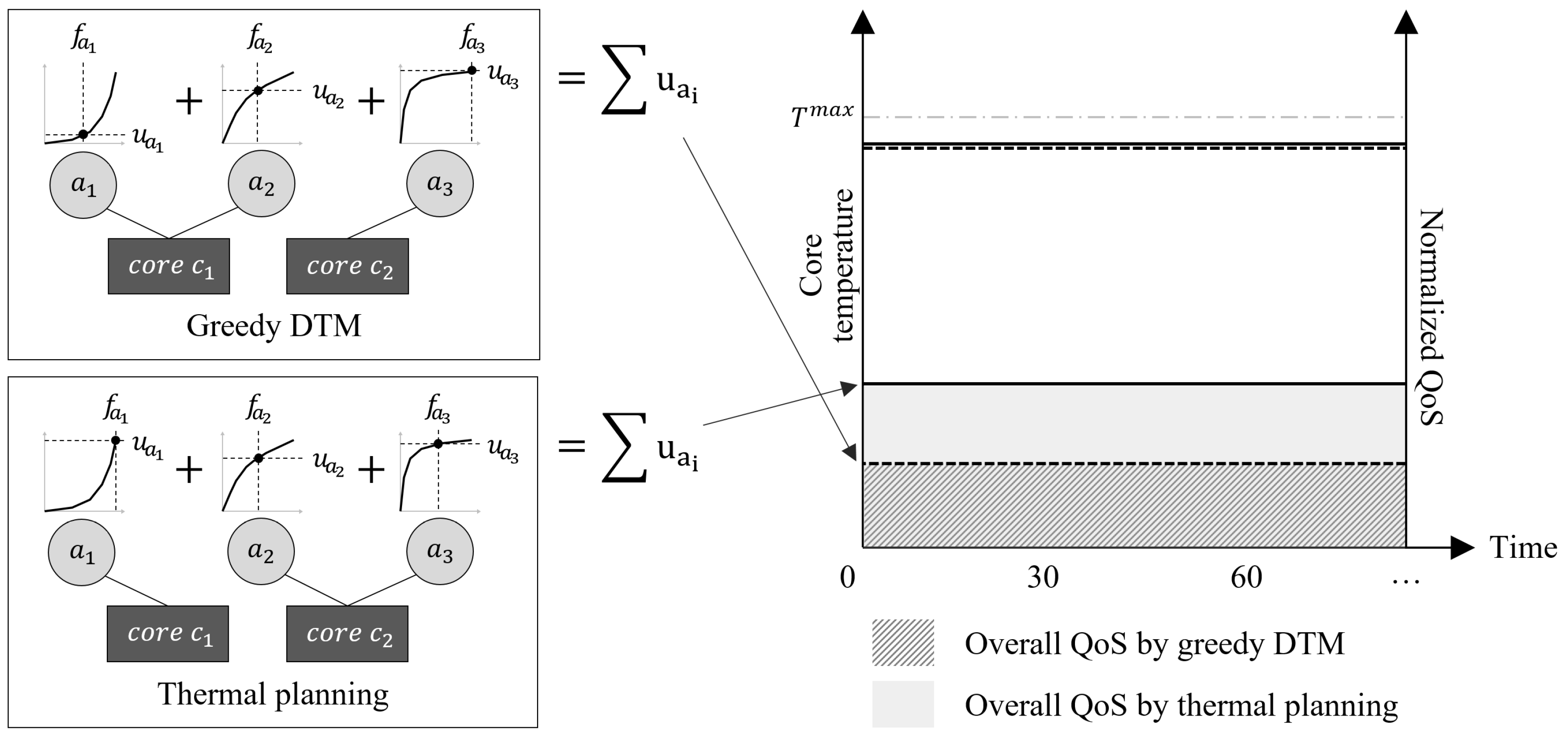
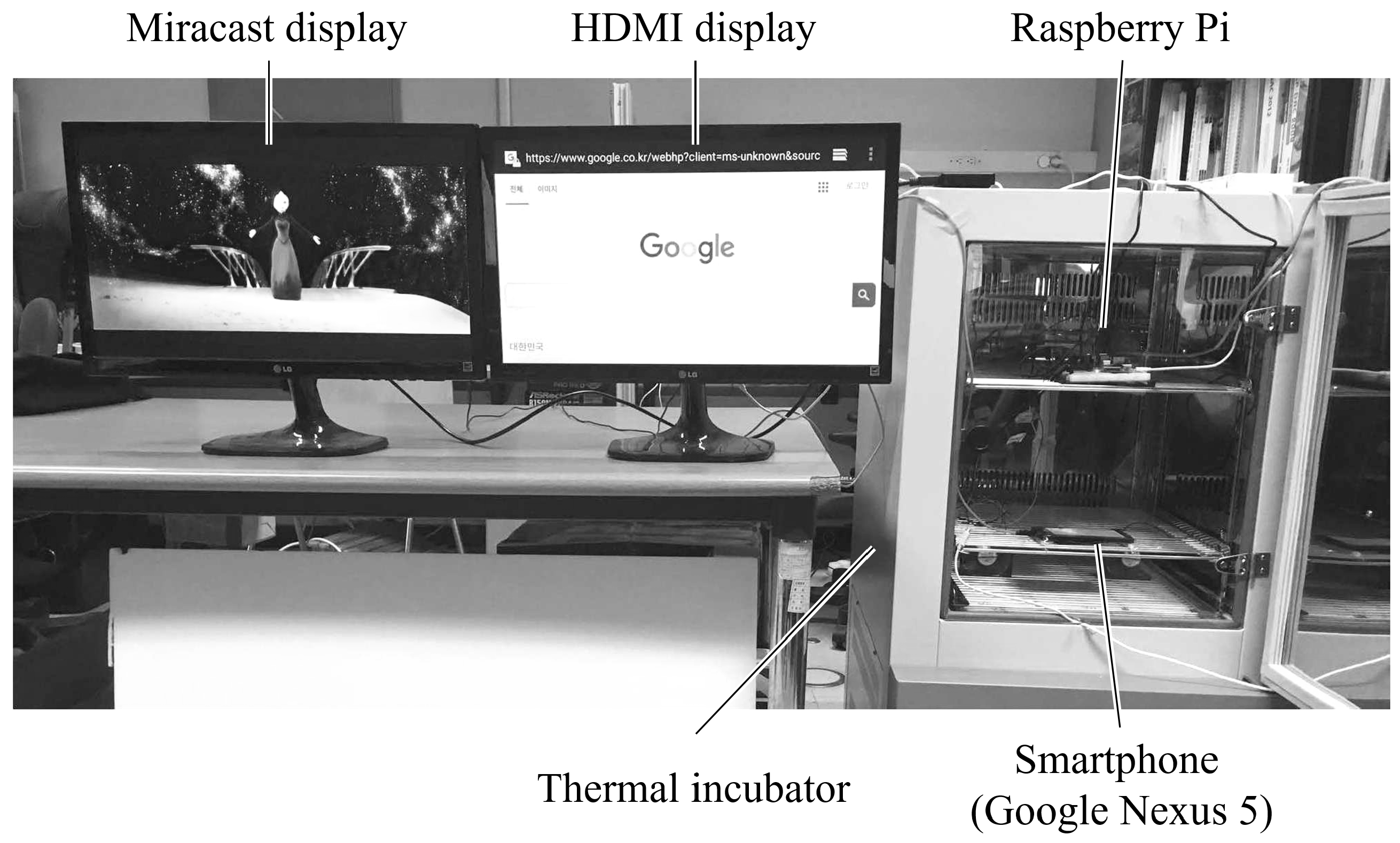
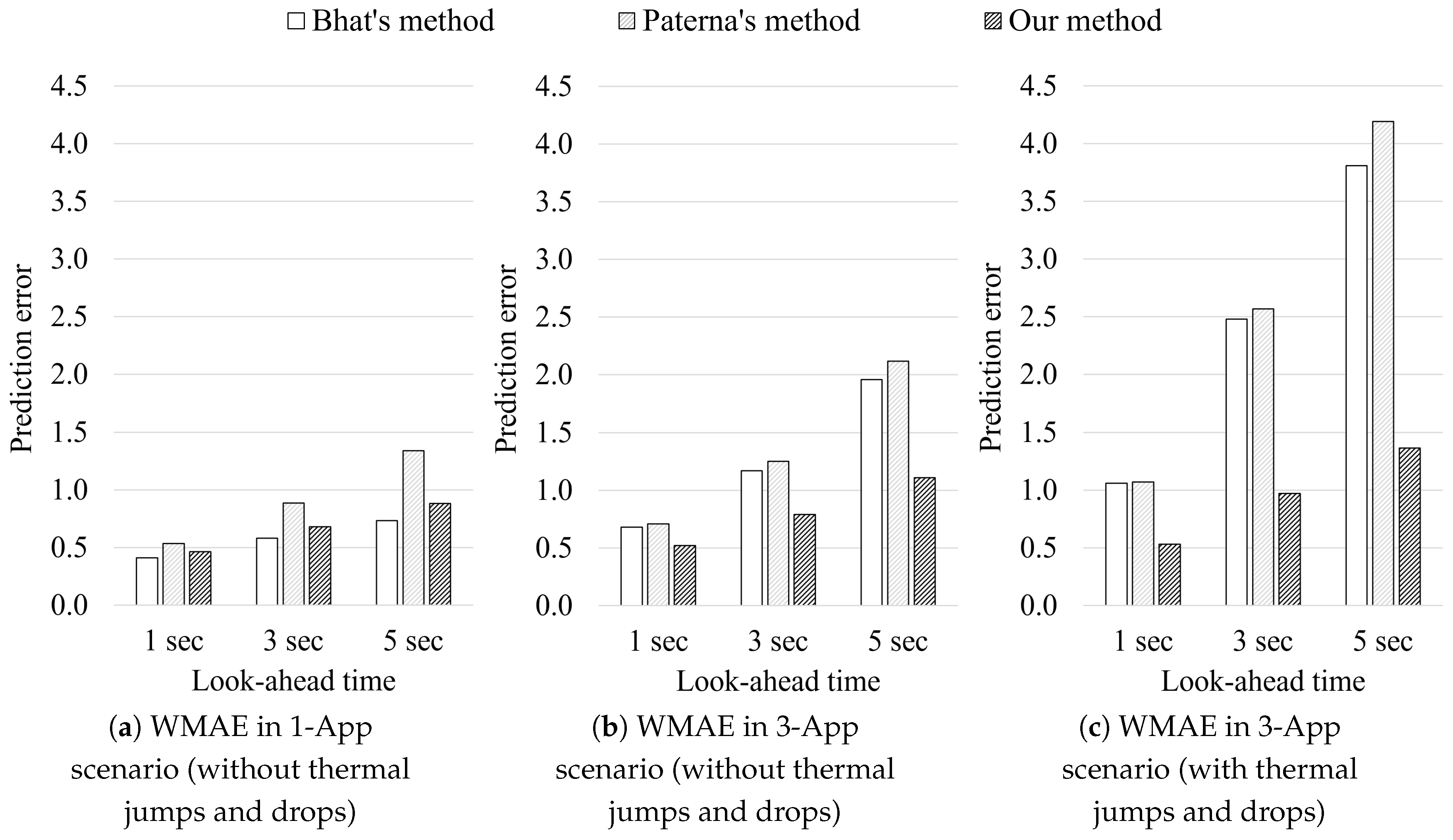
Table 1.
Comparison of detection results for 30 thermal violations.
| Type | Bhat’s Method | Paterna’s Method | Our Method |
|---|---|---|---|
| True positive | 23/30 (76.7%) | 9/30 (30.0%) | 29/30 (96.7%) |
| False positive | 0/1509 (0.0%) | 0/1509 (0.0%) | 0/1509 (0.0%) |
| True negative | 1509/1509 (100.0%) | 1509/1509 (100.0%) | 1509/1509 (100.0%) |
| False negative | 7/30 (23.3%) | 21/30 (70.0%) | 1/30 (3.3%) |
Table 2.
Categorization of the 9 applications used in our experiments.
| Category (QoS Metric) | Application | Description on QoS Metric |
|---|---|---|
| Execution-oriented (Execution time) | FFT | The time it takes to perform the FFT on randomly generated data 10,000 times |
| Matrix Multiplier | The time it takes to perform matrix multiplication on randomly generated matrices 10,000 times | |
| SHA256 | The time it takes to encrypt a randomly generated plain text with SHA256 10,000 times | |
| FPS-sensitive (FPS) | MXPlayer | FPS when the application plays a video file using hardware renderer |
| SlideShow | FPS when the application plays a slide show of randomly selected photos | |
| VLC Player | FPS when the application plays a video file using software renderer | |
| Response-sensitive (Response time) | SubwaySurf | The time it takes to load the application |
| Chrome | The page load time for http://m.naver.com | |
| The time it takes to load the application |
Table 3.
Comparison of average execution time of exhaustive-search-based algorithm and our algorithm.
Table 3.
Comparison of average execution time of exhaustive-search-based algorithm and our algorithm.
| Scenario Type | Exhaustive-Search Based Algorithm on PC | Our Algorithm on Smartphone |
|---|---|---|
| 3-App scenario | 2,818,969 ms (46 min) | 57 ms |
| 4-App scenario | 8,895,283 ms (148 min) | 120 ms |
| 5-App scenario | 23,399,420 ms (390 min) | 417 ms |
© 2018 by the authors. Licensee MDPI, Basel, Switzerland. This article is an open access article distributed under the terms and conditions of the Creative Commons Attribution (CC BY) license (http://creativecommons.org/licenses/by/4.0/).
Share and Cite
MDPI and ACS Style
Kwon, O.; Jang, W.; Kim, G.; Lee, C.-G. Optimal Planning of Dynamic Thermal Management for NANS (N-App N-Screen) Services. Electronics 2018, 7, 311. https://doi.org/10.3390/electronics7110311
AMA Style
Kwon O, Jang W, Kim G, Lee C-G. Optimal Planning of Dynamic Thermal Management for NANS (N-App N-Screen) Services. Electronics. 2018; 7(11):311. https://doi.org/10.3390/electronics7110311
Chicago/Turabian StyleKwon, Ohchul, Wonjae Jang, Giyeon Kim, and Chang-Gun Lee. 2018. "Optimal Planning of Dynamic Thermal Management for NANS (N-App N-Screen) Services" Electronics 7, no. 11: 311. https://doi.org/10.3390/electronics7110311
Note that from the first issue of 2016, this journal uses article numbers instead of page numbers. See further details here.