Multi-Object Detection in Traffic Scenes Based on Improved SSD

College of Field Engineering, PLA Army Engineering University, Nanjing 210007, China
*
Author to whom correspondence should be addressed.
Electronics 2018, 7(11), 302; https://doi.org/10.3390/electronics7110302
Submission received: 9 September 2018
/
Revised: 1 November 2018
/
Accepted: 2 November 2018
/
Published: 6 November 2018
(This article belongs to the Special Issue Machine Learning and Embedded Computing in Advanced Driver Assistance Systems (ADAS))
Abstract
:In order to solve the problem that, in complex and wide traffic scenes, the accuracy and speed of multi-object detection can hardly be balanced by the existing object detection algorithms that are based on deep learning and big data, we improve the object detection framework SSD (Single Shot Multi-box Detector) and propose a new detection framework AP-SSD (Adaptive Perceive). We design a feature extraction convolution kernel library composed of multi-shape Gabor and color Gabor and then we train and screen the optimal feature extraction convolution kernel to replace the low-level convolution kernel of the original network to improve the detection accuracy. After that, we combine the single image detection framework with convolution long-term and short-term memory networks and by using the Bottle Neck-LSTM memory layer to refine and propagate the feature mapping between frames, we realize the temporal association of network frame-level information, reduce the calculation cost, succeed in tracking and identifying the targets affected by strong interference in video and reduce the missed alarm rate and false alarm rate by adding an adaptive threshold strategy. Moreover, we design a dynamic region amplification network framework to improve the detection and recognition accuracy of low-resolution small objects. Therefore, experiments on the improved AP-SSD show that this new algorithm can achieve better detection results when small objects, multiple objects, cluttered background and large-area occlusion are involved, thus ensuring this algorithm a good engineering application prospect.
1. Introduction
Pedestrian and vehicle object detection and recognition in traffic scenes is not only an important branch of object detection technology but also the core technology in the research fields of automatic driving, robot and intelligent video surveillance, both of which highlights its significance in research [1].
The object detection algorithm based on deep learning can be applied to a variety of detection scenarios [2], mainly because of its strong comprehensiveness, activeness and capability of detecting and identifying multiple types of objects simultaneously [3,4,5,6]. Among various types of artificial neural network structures, deep convolutional networks, with powerful feature extraction capabilities, have achieved satisfactory results in visual tasks such as image recognition, image segmentation, object detection and scene classification [7].
Faster R-CNN (where R corresponds to “Region”) [8] is the best method based on deep learning R-CNN series object detection. By using VOC2007 + 2012 training set, the VOC2007 test set tests mAP to 73.2% and the object detection speed can reach 5 frames per second. Technically, the RPN [8] network and the Fast R-CNN network are combined and the proposal acquired by the RPN is directly connected to the ROI (Region of interest) pooling layer, which is a framework for implementing end-to-end object detection in the CNN network.
YOLO (You Only Look Once) [9] is a new object detection method, which is characterized by fast detection and high accuracy. Its author considers the object detection task as a regression problem for object area prediction and category prediction. This method uses a single neural network to directly predict item boundaries and class probabilities, thus rendering end-to-end item detection possible. With its detection speed fast enough, YOLO’s basic version can achieve real-time detection of 45 frames/s and the Fast-YOLO can reach 155 frames/s. In comparison with other object detection systems that exist currently, the YOLO object area has a larger positioning error but its false positive of the background prediction is better than the currently existing ones of other systems.
SSD, the abbreviation for Single Shot Multi-box Detector [7], is an object detection algorithm proposed by Wei Liu on ECCV 2016 and is one of the most-often used detection frameworks so far. In comparison with Faster-RCNN [8], it is much faster; and in comparison with YOLO [9], it has a more satisfactory accuracy mean (MAP). Generally speaking, SSD has the following main characteristics:
- (1)
- It incorporates YOLO’s innovative idea of transforming detection into regression, thus making it possible to complete network training at one time;
- (2)
- Based on the Anchor in Faster RCNN, it proposes a similar Prior box;
- (3)
- It incorporates a detection method based on the Pyramid Feature Hierarchy, with similar ideas to those of FPN.
Although SSD has achieved higher accuracy and better real-time performance on specific data sets, the training process of the model is not only time-consuming but also heavily dependent on the quality and quantity of training samples. The object is detected by the color and edge information of the image, which undermines the detection effects of those objects that do not have enough image information, particularly when small and weak objects and large-area occlusion of objects are involved. The detection efficiency of the algorithm still needs to be improved to meet the real-time requirements of equipment operation.
According to the characteristics and requirements of pedestrian and vehicle object detection tasks in complex traffic scenes, the following four improvements have been made to the traditional SSD algorithm:
(1) Inspired by the shape of the primary feature convolution kernel which is trained by the deep neural network, we take into account human visual characteristics so as to design and construct a Gabor feature convolution kernel library which is composed of multi-scale Gabor, multi-form Gabor and color Gabor. Aiming at the multi-object self-characteristics to be detected in traffic scenes, we get the optimal feature extraction Gabor convolution kernel set through training and screening and this set is to replace the low-level convolution kernel set which is used by the original feature extraction network model VGG-NET (Visual Geometry Group) for regional basic feature extraction, thus we obtain a new feature extraction network Gabor-VGGNET, which greatly enhances SSD’s ability to distinguish multi-object;
(2) In order to solve the problem that SSD has difficulty in detecting small and weak objects with low resolution in large traffic scenes, a dynamic region zoom-in network (DRZN) is proposed after we use enhanced learning and sequential search methods and consider those characteristics and requirements of object detection tasks in large traffic scenes. The network framework greatly reduces the amount of computation by down-sampling images and maintains the detection accuracy of objects with different sizes in high resolution images through dynamic region zoom-in, thus improving significantly the detection and identification accuracy of small and weak objects with low resolution and reducing the missed-alarm rate;
(3) The traditional SSD has the defect that the fixed confidence threshold is not flexible enough. Therefore, the fuzzy threshold method is used here to employ the adaptive threshold strategy so as to reduce the missed-alarm rate and the false alarm rate;
(4) In order to realize real-time video object detection on low-power mobile and embedded devices, a single-image multi-object detection framework is combined with a Long Short Term Memory (LSTM) network to form an interleaved circular convolution which realizes the temporal correlation of network frame level information by using an efficient Bottleneck-LSTM layer to refine and propagate the feature mapping between frames and greatly reduces the network computing cost. Using the timing correlation feature of LSTM and the dynamic Kalman filter algorithm, we can track and recognize the object affected by strong interference such as illumination variation and large-area occlusion.
2. Improved Feature Extraction Network Gabor-VGGnet
2.1. Gabor Convolution Kernel Design by Simulating Photoreceptive Cells
Convolutional neural net-work [10] is a special deep neural network model. Its particularity is embodied in two aspects. On the one hand, its connections between neurons are not fully connected and on the other hand, some neurons are in the same layer which means that the weights of the connections are shared (i.e., the same). Its network structure of non-full connection and weight-sharing makes it more similar to biological neural networks, which reduces the complexity of the network model and reduces the number of weights [10].
Deep convolution neural network can combine feature extraction with recognition and can be optimized continuously through back propagation, thus making feature extraction a self-learning process that avoids the limitations caused by manual feature selection. Training a certain convolution layer of the deep convolution neural network is actually training a series of filters to activate these filters’ high sensitivity to specific objects and in so doing we can recognize and detect the deep convolution neural network. The filter bank of the first convolution layer of the convolution neural network is used to detect low-order features. With the increase of convolution layer, the features detected by the corresponding filters are more complex. At the beginning of the training, the filters of the convolution layer are completely random and they will not activate any features, that is, they will not be able to detect any features [11]. Then, through the deep convolution neural network visualization toolbox “Yo shin ski/Deep-Visualization-Toolbox” [12], we can obtain the feature convolution kernels of each level by visualizing the CNN model, all of which can be shown in the following Figure 1:
The Gabor wavelet is similar to the visual stimulus response of simple cells in the human visual system. It has good characteristics in extracting the local spatial and frequency domain feature information of the object and has strong robustness to the change of the brightness and contrast of the image as well as to the change of the object attitude. Moreover, it demonstrates the most useful local features for object recognition, which is mainly why it is widely used in computer vision and texture analysis. Compared with other methods, Gabor wavelet transform can deal with fewer data to meet the real-time requirements of the system; on the other hand, wavelet transform is insensitive to light changes and can tolerate a certain degree of image rotation and deformation, both contribute to the improved robustness of the system [13].
In the airspace, a 2-dimensional Gabor filter is the product of a sinusoidal plane wave and a Gaussian kernel function. Gabor filters are self-similar, that is, all Gabor filters can be generated from expansion and rotation of a mother wavelet. Traditional Gabor filters extract relevant features in different directions in different frequency domains. However, when it is practically applied, we found that the two-dimensional Gabor function can enhance the edge and the underlying image features such as peak, valley and ridge contours. The mathematical expression of the two-dimensional Gabor function is shown in Equation (1), Equation (2) is the real part of the function and Equation (3) is the imaginary part of the function.
In the equation, x and y represent the abscissa and ordinate of this pixel, x’ = xcosθ + ysinθ, y’ = −xsinθ + ycosθ, λ1 represents the sine function wavelength; θ1 represents the direction of the kernel function; ψ1 represents the phase shift; σ2 represents the standard deviation of the Gaussian function; γ1 represents the aspect ratio of the space. The real part can smooth the image and the imaginary part can be used for edge detection. The schematic diagram of the real part of the filter is shown in Figure 2, where the left side is the real component and the right side is the imaginary component.
Traditional convolution kernels are generally rectangular or square in shape but our experiments generate the finding that the shape of the Gabor filter convolution kernel has a decisive influence on the edge enhancement effect of the Gabor filter. Each of those different-structured Gabor filters can form an optimal response to the image content that is consistent with its scale, direction, center position, phase and structure type. In order to enable the Gabor filter to extract more complex and rich edge and texture feature information, we introduce parameters k1, k2, k3, k4 and k5 to adjust the Gabor convolution verification part, as shown in Equation (4).
Figure 3 shows the partial two-dimensional Gabor filter convolution kernel constructed by Equation (4). The parameters k2, k3 and k5 determine the structure type of the convolution kernel. The parameters k1 and k4 determine the direction of the Gabor filter convolution kernel and thereby extract more complex and rich information on edge and texture feature
Compared with other visual features, color features require less computation and depend less on the viewing angle, direction and size of the image, thereby they have better robustness and lower complexity. RGB space is currently the most commonly used way to express color information. It uses the brightness of the three primary colors of red, green and blue to quantitatively express color and uses R (red), G (green) and B (blue) three-color lights to superimpose each other to realize color mixing. If the proportion of the three colors is different, the colors obtained will be different. The traditional Gabor filter is only used to extract edge, texture and other features from gray images, thus ignoring the color information that plays an important role in image object detection. Inspired by the color convolution kernel trained by the deep convolution neural network, we use the color convolution kernel trained by the neural network as a reference to construct a three-dimensional color Gabor filter through reconstruction to activate the color features of color images.
There are three different kinds of cone cells in the eye, which are sensitive to light of red, green and blue wavelengths respectively. When light waves of different wavelengths enter the eye and are projected on the retina, the brain perceives the color of the scene by analyzing the information input by each cone cell [14]. Imitating the visual mechanism of human eyes, we take a two-dimensional Gabor filter to filter the color feature detection of one color component in a three-dimensional color space, then we construct the relationship among the three color components according to the color characteristics of the object to be extracted and finally we obtain Gabor filters of the other two color components respectively. By combining these three two-dimensional filters [15,16], we can obtain a color Gabor filter too extract the specified object color features.
In Equation (5), gbR represents a two-dimensional Gabor filter of color Gabor on the R color channel and the shape of the gbR convolution kernel is determined by the above formula. gbG and gbB are two-dimensional Gabor filters of color Gabor on G and B color channels, respectively. In the acknowledged receptive field, there are four components: red, green, blue and yellow, with four receptive fields [17]. In order to imitate the perception of color by human visual cells, we use the color convolution kernel trained by neural network as a reference and summarize the mathematical relationship between each color channel by imitation and reconstruction, as is shown in Equations (6) and (7):
The constraint behind Equation (7) is the color Gabor-sensitive object color. For example, R&G indicates that the object primary color is red and green and Y represents yellow. Figure 4 shows a partial color Gabor convolution kernel:
2.2. Intelligent Screening Process for Optimal Gabor Convolution Kernel Set
In the experiment, we use vehicle objects datasets to train the SSD512 [7] model and then assess the convolution kernels’ influence on the object recognition rate when the number of convolution kernels vary. After analyzing the experimental results, we set the depth of the convolution layer to be 128 → 256 → 384 → 384 → 384 respectively in order to ensure the highest possible detection accuracy. In the human retina, there are about 6 million to 8 million cone cells and the total number of rod cells is more than 100 million. The ratio of the two is about 10:1 [14]. Therefore, we set the number of two-dimensional Gabor convolution kernels in the first layer of Gabor convolution core group to be 110 and the number of color Gabor convolution kernels to be 18. Then we use the vehicle object dataset in the KITTI dataset [15] to train several different convolution kernels and test their influence on the recognition rate. Through the experiment, we find that the two-dimensional Gabor filter convolution kernel is 3 × 3 in size, the color Gabor filter convolution kernel is 5 × 5 and when the 1 × 1 convolution kernel is added to the Inception structure of the network for dimensionality reduction, the combined filter bank can obtain better object feature sensitivity. In order to effectively improve the detection accuracy of the algorithm as a whole, it is important to construct a reasonable Gabor feature extraction convolution kernel group to extract multiple features with different degrees of discrimination. The screening process of the optimal Gabor convolution kernel group is shown in Figure 5.
First, a two-dimensional Gabor library containing various forms is constructed by means of transforming parameters from Equations (1) and (4); a color Gabor library of the same size can be constructed from Equations (6) and (7); and then a small-scale test image set containing only “people,” “riders” and “vehicles” respectively (20 for each of the three objects, 60 in total) is constructed. Convolution kernels are randomly and non-repeatedly extracted from two Gabor libraries to form convolution kernel groups; each convolution kernel group rolls up the images of the test set one by one and then corresponding feature maps can be obtained through non-maximum suppression. Then we convert the feature maps into feature vectors through pooling and input the soft max classifier, a traditional SSD detection framework that has trained with small sample data. Thus we can obtain the detection confidence of the test image object and with it we take the average of all confidence of the test set as the evaluation score for the feature extraction effectiveness of the convolution kernel group, so that we obtain the optimal convolution kernel group which is corresponding to the highest evaluation score.
The scale of Gabor library is reasonably determined by the actual number of convolution kernels in the convolution kernel group. If the scale of Gabor library is too large, then he calculation amount is too large and if it is too small, then it is not representative and the information is not comprehensive enough. The combination of m1 convolution kernels from the library with a total number n1 is shown in Equation (8)
In order to avoid the data explosion caused by too many combinations and the incompleteness of feature extraction caused by the small-sized database, we randomly divide two-dimensional Gabor convolution kernels into 2 groups each with 10 convolution kernel inside and then divide color Gabor convolution kernels into 2 groups each with 18 convolution kernel inside. The scale of the constructed Gabor library is 180 convolution kernels
3. Improvement of Small and Low-Resolution Object Detection Problem
The SSD adopts the feature pyramid structure for detection and has good detection accuracy for small and weak objects. However, the detection effect for low-resolution and weak objects in complex and large traffic scenarios is still not ideal [7].
In order to solve the problem that the existing SSD is difficult to detect small and weak objects with low resolution in complex large scenes, this paper proposes a dynamic region zoom-in network (DRZN), which reduces the calculation of object detection by down-sampling the images of high resolution large scenes while maintaining the detection accuracy of small and weak objects with low resolution in high resolution images through dynamic region zoom and the effect of improving the detection and recognition accuracy is obvious. The detection is performed in a coarse-to-fine manner. First, the down-sampled version of the image is detected and then the areas identified as likely to improve the detection accuracy are sequentially enlarged to higher resolution versions and then detected. The method is based on enhanced learning and consists of an amplification precision gain regression network [16] (R-net) and a Zoom-in region selection algorithm. The former learns the correlation between coarse detection and fine detection and predicts the precision gain after region amplification and the latter performs learning and predicts the result before it dynamically selects regions to be amplified.
First, the down-sampled version of the image is roughly detected in order to reduce the amount of computation and to improve the operation efficiency. Then, the regions where low-resolution small objects may exist are sequentially selected for amplification and for analysis to ensure the recognition accuracy of the low-resolution small objects. We use the reinforcement learning method to model the amplification reward in terms of detection accuracy and calculation efficiency and then we dynamically select a series of regions to be amplified to high resolution for analysis. Reinforcement learning (RL) is a branch of machine learning. Compared with the typical problems generated from supervised-learning and unsupervised-learning of machine learning, the biggest feature of reinforcement learning is learning from interaction. In the interaction between agent and environment, agent learns knowledge continuously as it is motivated by the reward or punishment obtained and adapts to the environment more. The RL learning paradigm is very similar to our human learning process and therefore RL is regarded as an important way to achieve universal AI.
RL is a popular mechanism for learning sequential search policies, as it allows models to consider the effect of a sequence of actions rather than individual ones. The current machine learning algorithms can be divided into three types: supervised learning, unsupervised learning and reinforcement learning.
In many other machine-learning algorithms, the learner is just learning how to do, while RL can learn which action to choose so as to get the maximum reward in a specific situation. In many scenarios, the current action will not only affect the current rewards but also affect the subsequent status and a series of rewards.
The three most important characteristics of RL are:
- (1)
- It is usually a closed-loop form;
- (2)
- It does not directly indicate which actions to choose;
- (3)
- A series of actions and reward signals will affect the action that follows. Existing works have proposed methods to apply RL in cost sensitive settings. We follow the approach and treat the reward function as a linear combination of accuracy and cost.
The overall framework of the algorithm is shown in Figure 6.
The algorithm mainly consists of two mechanisms: (1) the first one is to learn the statistical relationship between the coarse detector and the fine detector, so as to predict which areas need to be amplified with the given output of the coarse detector; (2) The second mechanism is to analyze the sequence of regions at high resolution when the coarse detector output and the region that needs to be analyzed by the fine detector are already given.
The strategy proposed and used in this paper can be expressed as a Markov decision process [17]. At each step, the system first observes the current state, estimates the potential cost-perceived rewards for different actions and selects actions with the greatest long-term cost-perceived rewards. The elements include: action, state set, cost-aware reward.
Action. The algorithm analyzes regions with high magnification returns in high resolution. Here, the action refers specifically to the selection of an area to be analyzed with high resolution. Each action can be represented by a vector , among which represents the location of the specified area and indicates the size of the specified area. In each step, the algorithm make assessment of a set of potential actions (list of rectangular regions) based on potential long-term rewards.
State set. It represents the encoding of two types of information: the prediction accuracy gain of the area to be analyzed and the history of the area that has been analyzed with high resolution (the same area should not be amplified by multiple times). We design an amplification precision gain regression network (R-net) to learn the information accuracy gain map (AG map) as a representation of the state. The AG map has the same width and height as the input image. The value of each pixel in the AG map is an estimation of how much detection accuracy can be improved by including that pixel in the input image. Therefore, the AG map provides a detection accuracy gain for selecting different actions. After the action is taken, the value corresponding to the selected region in the AG map is correspondingly reduced, so the AG map can dynamically record the action history.
Cost-aware reward. The state encodes the prediction accuracy gain when the amplification of every image sub-region is involved. In order to maintain high precision with a limited amount of computation, we define a loss-return function, as Equation (9) shows. Given the state and action, the loss-reward function scores each action (zoom area) by considering cost increments and precision improvements.
Here, k in the action indicates that the object k is included in the region selected by the action, and indicates the object detection score for the same object coarse detector and fine detector and is the corresponding object real label. The variable represents the total number of pixels in the selected area, representing the total number of pixels in the input image. The first term in the formula indicates an increase in detection accuracy. The second term indicates the cost of amplification. The balance between accuracy and calculation is controlled by parameters.
The Amplified Precision Gain Regression Network (R-Net) predicts the precision gain of amplification over a particular region based on the coarse detection results. R-Net trains on the coarse and fine test data pairs so that it can observe how they relate to each other in order to learn the appropriate precision gain relationship [7].
The two SSDs are trained respectively on a high resolution fine image training set and on a low resolution coarse image training set and then it is used as coarse and fine detectors respectively. We apply two pre-trained detectors to a set of training images and obtain two sets of image detection results: low resolution detection in down-sampled images and high resolution detection in high resolution versions of each image. Here, d is the detection bounding box, p is the probability of being the object and f is the corresponding detected feature vector. We use the superscripts h (High) and l (Low) to represent high resolution and low resolution (down-sampled) images.
In order to enable the model to differentiate whether or not the high-resolution detection can improve the overall detection result, we introduce a matching layer to correlate the detection results produced by the two detectors. In this layer, if we find that the possible object in the down-sampled image and the possible object in the high resolution image have a sufficiently large intersection (), then the definitions of i and j correspond with each other. We match the rough detection scheme and the fine detection scheme according to the rules and thus generate a set of correspondence between them [7].
Given a set of correspondences , we can estimate the amplification accuracy gain of the coarse detection. The detector can only handle objects within a certain range, so applying the detector to a high resolution image does not necessary produce the best accuracy. For example, if the detector is primarily trained on a small object dataset, the detection accuracy of the detector for larger objects is not high. Therefore, we use to measure which test result (rough or fine) is closer to the fact and in the equation is a measure of the real tag. When the high resolution score is closer to the basic fact than the low resolution score, the function indicates that the object is worth zooming in. Otherwise, applying a coarse detector on the down-sampled image may result in higher precision, so we should avoid zooming in on the object. We use the correlation regression (CR) layer to estimate the amplification accuracy gain of the object K, such as Equation (10).
Here, ϕ represents the regression function and W1 represents the parameter set. The output of this layer is the estimated accuracy gain. The CR layer consists of two fully connected layers, with 4096 cells in the first layer and only 1 output cell in the second layer.
An AG map (Accuracy Gain map) can be generated based on the learning accuracy gain of each object. We assume that each pixel within the candidate frame has an equal contribution to its accuracy gain. Therefore, the AG map generated is:
In Equation (11), indicates that the point is within the bounding box , indicates the number of pixels contained in . Is a constant and indicates the estimated parameters of the CR layer. The AG map is used as a state representation, which naturally contains information about the quality of the rough detection. After zooming in and detecting the area, all values in the area are set to be 0 so as to prevent future scaling in the same area. The R-net structure of the amplification precision gain regression network is shown in Figure 7.
Through R-net we obtain the AG map and the value of each pixel in the AG map is an estimate of how much detection accuracy can be improved by including that pixel in the input image. Therefore, the AG map provides a detection accuracy gain for the selection of different actions. After the action is taken, the value corresponding to the selected region in the AG map is correspondingly reduced, so the AG map can dynamically record the action history. According to AG map, we propose a dynamic zooming region selection algorithm. The specific algorithm flow is shown in Figure 8.
Firstly, we divide the AG map into equal-area rectangular regions according to the 8 × 8 grid, count the sum of the pixel values in each rectangle, set the threshold and select the regional center block. The 3 × 3 rectangles that center on the center block of each region constitute the enlarged screening area. If an enlarged screening area has several rectangular regions that satisfy the threshold value of the pixel value, then the one with the largest pixel value is taken as the center of the region. If the center of the region is taken on the side of the large square, the 3 × 3 is formed by adding blank squares of the same size. In the enlargement and screening area, we take the central point of enlarged screening area as the center. Then four prediction bound boxes with different ratios of length, width and breadth are constructed and the best enlargement area bounding box can be selected after we compare the structural indicators (pixel values, ratios) of each prediction bounding box.
The total pixel value sumpxi in the rectangular area rtgi in the grid-divided AG map is shown in Equation (12).
Here, the pxj represents the pixel value of the jth pixel in the rtgi region. The larger the sumpxi value, the larger the amplification gain of the rectangular region rtgi and the region with high magnification gain is taken as the center to make it correspond to the human eye’s processing of the block domain. We adaptively select the pixel value threshold by the second-order difference method to complete the initial screening of the regional center block. The second-order difference can represent the magnitude of the change in the discrete array and can be used to determine the threshold in a set of pixel values. By detecting an AG map, 64 candidate regions are obtained by default. Finally, each candidate region obtains an overall pixel value sumpxi for indicating the amplification gain. Therefore, a total of 64 × 1 arrays can be obtained and elements less than 0.1 are discarded. To have no object, get an n × 1 array C. Let the function of estimating the slope of the sumpxi from decreasing by f (g), see Equation (13).
Then, take the Ck as the sumpxi threshold of the AG map image and this Ck is obtained when f (Ck) takes the maximum value.
In order to reduce the calculation amount of area enlargement and fine detection, to effectively improve the efficiency and real-time of the algorithm and to ensure the better tolerance of the selected area, we form an enlarged screening area with 3 × 3 rectangles centering on each regional central block. If the same zoom-in filter area has multiple rectangular areas that satisfy the pixel value threshold condition, the one with the largest pixel value is taken as the center of the area.
We use the center point of the enlarged screening area as the center position to predict the prediction bounding boxes of six fixed sizes according to different aspect ratios. The area of the enlarged screening area is SZ. The area of each predicted bounding box is shown in Equation (14).
Here, smin = 0.1 × SZ, smax = 0.7 × SZ, m = 5. We give different aspect ratios for different prediction bounding boxes, such as Equation (15).
In the equation, W and H respectively indicate the width and length of the bounding box. Then, the width and length of the bounding box are predicted to be , respectively. When ar = 1, there is also a prediction bounding box with a scale of 6, that is, , so there are a total number of 6 prediction bounding boxes. For any bounding box, bl, we calculate the total pixel value in the box sumpxi, such as Equation (16).
W and L represent the width and length of the box respectively. The proportion P of pixels with high amplification income in the region bl is shown in Equation (18):
Pn1 represents the total number of pixels in the bl region with pixel gains (pixel values with pixel values greater than 0.1) and Pn2 represents the total number of pixel points in the bl region. That is, for each prediction bounding box, bl has a feature vector (x, y, sumpxi, W, L, P) and x and y respectively represent the abscissa and ordinate of the center point of bl.
We use a manually calibrated training sample to train a Logistic classifier [18] to evaluate the frame selection effect of each prediction bounding box. We classify the evaluation results into two categories: a prediction bounding box that satisfies the amplification requirements and a prediction bounding box that does not meet the amplification requirements.
For the input prediction bounding box, bl (x, y, sumpxi, W, L, P), Logistic classifier introduces weight parameter θ = (θ1, θ2, …, θ6), then weights the attributes in bl to obtain θTbl and then it introduces a logistic function (sigmoid function) to get the function hθ(bl), as is shown in Equation (19):
Thus, we get the estimation function , as is shown in Equation (20):
It means the probability that the label is y when the test sample bl and the parameter θ are determined.
After evaluating the frame selection effect of each prediction bounding box by Logistic classifier, we can obtain a corresponding frame selection evaluation score for each prediction bounding box and then perform a non-maximum value suppression to obtain the final prediction as the final Enlarged bounding box.
After completing the selection of the enlarging bounding box, we set all the pixel values in the enlarged screening area to 0 so as to avoid the inefficiency caused by repeated selection. Then we update the corresponding area of the AG map and detect whether the AG map has been highly enlarged profit area for detection (whether the total value of the AG map pixel is 0) has been detected; if yes, then we complete the detection, if no, then we continue to repeat the detection process.
Before the original image of the obtained fine detection candidate region is sent to the fine detector for detection, the bilinear interpolation is first performed to be enlarged to the minimum size of the candidate detection region of fine detector detection (This paper sets the minimum candidate region to be 10 × 10).
4. Confidence Determination by Adaptive Threshold
In the final stage of SSD classification, we use Soft-max to classify the candidate region which will obtain the confidence level (i.e., the probability of belonging to each category) belonging to each category. When the confidence level belonging to a certain class is higher than the set threshold, the candidate region is used. It is judged as the object of this kind and if the same candidate area has multiple categories whose confidence level is higher than the threshold, the highest one is taken [19]. Aiming at the insufficiency of SSD to detect the fixed confidence threshold, the fuzzy adaptive threshold method [20] is used to make adjustment to the adaptive threshold strategy so as to reduce the missed alarm rate and false alarm rate.
The fuzzy degree is determined by the fuzzy rate function. When the fuzzy rate is the lowest, the segmentation effect is the best. Among them, the fuzzy rate is related to the membership function and the basic idea of fuzzy mathematics is the idea of membership degree [18]. By default, N candidate regions obtained by detecting an image are sent to SSD and finally M confidence levels are obtained for each candidate region to represent M categories. So N arrays of M × 1 size can be obtained altogether. The maximum value in each array is taken out and sorted from large to small and the values less than 0.1 among them are discarded (if all the n values are less than 0.1, it is determined that there is no object), resulting in an array C of n × 1. μ(x) is the membership function and μ(Ck) is the membership of the region in the array C where the confidence level is Ck. The ambiguity rate γ(C) of array C is the ambiguity measure parameter for array C. Here h(Ck) represents the number of elements in the array C whose confidence is Ck and the ambiguity rate γ(C) of the array C is defined in Equation (21).
In this equation, the ambiguity rate γ(C) of the array C depends on the membership function μ(x).
Then μ(x) is determined by the window width c = 2∆q and the parameter q. Once the window width is selected, γ(C) is only related to the parameter q. The solution process of the fuzzy threshold method is to preset the window width and the coefficient is often set to be 0.3. By changing q to make the membership function μ(x) slide over the confidence interval [C0, Cn−1], the blur rate curve is obtained by calculating the blur rate γq(C), the valley point of the curve is q that makes γq(C) get a minimum value, which is the adaptive threshold value.
5. Video Multi-Object Detection Technology Based on Recurrent Neural Network
This section examines strategies for building video detection models by increasing time perception while the operating speed and low computational resource consumption are both ensured. Video image data contains a variety of time cues that can be expanded to achieve more accurate and stable object detection than a single image. Therefore, the detection result information from the earlier frame can be used to refine the prediction result at the current frame. Since the network can detect objects in different states across frames, the network prediction results will also have higher confidence as the training time progresses, thus effectively reducing the instability in single image object detection.
In order to realize real-time video object detection on low-power mobile and embedded devices, a single-image multi-object detection framework is combined with a Long Short Term Memory (LSTM) network to form an interleaved circular volume. The product structure, by using an efficient Bottleneck-LSTM layer [21] to refine and propagate the feature mapping between frames, achieves the temporal correlation of network frame-level information and greatly reduces the network computing cost. By using the timing correlation feature of LSTM and the dynamic Kalman filter algorithm [22], we can track and recognize the object affected by strong illumination and large-area occlusion in the video is realized.
The Recurrent Neural Network (RNN) solves this problem better. They are networks with loops that allow information to persist. One of the advantages of RNN is that they can relate previous information to current tasks, such as using previous video frames to help detect current video frame [23]. Long-Short Term Memory (LSTM) is a special RNN designed to avoid long-term dependencies. A method of combining convolutional LSTMs into a single image detection framework is proposed as a means of propagating frame level information across time. However, the simple integration of LSTMs leads to a large amount of computation and prevents the network from running in real time. To solve this problem, a Bottleneck-LSTM was introduced, which uses the features of deep separable convolution and Bottleneck design principles to reduce computational costs. Figure 9 shows the network structure of the LSTM-SSD. Multiple convolutional LSTM layers are inserted into the network, each of which propagates and refines the feature map according to a certain proportion.
A layer of Conv-LSTM in the network receives the feature map of its previous Conv-LSTM and then we form a new feature map by combining the current map obtained in the above process with the one transmitted from the previous frame and then we predicts the detection result and transmits the feature map to the following Conv-LSTM and convolution layer. The output of Conv-LSTM will replace all the previous feature maps in all subsequent calculations and continue the detection task. However, the simple integration of LSTMs can lead to a large amount of computation and thus prevents the network from running in real time. To solve this problem, we introduce a Bottleneck-LSTM that takes advantage of its deep separable convolution as well as of the Bottleneck design principles to reduce computational costs.
The video data is regarded as a sequence V composed of multiple frames of images, The task of the algorithm is to obtain the frame-level detection result D, , Dk represents the detection result of the image frame Ik, which includes the position of a series of detection frames and the recognition confidence of each object. We consider constructing an online learning mechanism so that the detection result Dk can be predicted and corrected by the image frame Ik−1, such as Equation (23)
Here refers to the vector of feature maps which describes the image of the kth frame of the video; represents an AG map describing the image of the kth frame of the video. We can construct a neural network with m layer LSTM convolution layer to approximately realize this function. This neural network takes each feature map and amplification precision enhancement map AGt−1 in the feature map vector st−1 as the input of LSTM convolution layer and thus we can obtain the corresponding feature map vector st and amplification precision enhancement map AGt. If we want to get the detection result of the whole video, we only need to run each frame of image sequentially through the network.
When applied to video sequences, the LSTM state can be understood as a feature representing timing. LSTM can then refine its input using timing features at each timing step and meanwhile it can extract additional time information from the input and updating its status. This refinement pattern can be applied by placing LSTM convolution layers immediately on any intermediate feature map. The feature map is used as the input to LSTM and the output of LSTM will replace the previous feature map in all subsequent calculations. The single frame image object detector can be defined by a function G (It) = Dt, which will be used to construct a composite network with m LSTM layers. These LSTM convolution layers can be considered as dividing the layer of function G into m + 1 suitable sub-networks , then such as Equation (24)
The “” represents the Hadamard product. We also define any layer of LSTM convolutional layer into a function.
In Equation (25), M and M+ are feature maps of the same dimension. Then we calculate the formula according to the timing as Equation (26):
Figure 10 depicts the input and output of the entire model when video is processed.
Because multiple gates need to be computed in a single forward channel, LSTMs have high requirements for computing resources, which greatly affects the overall efficiency of the network. To solve this problem, a series of changes have been introduced to make LSTMs compatible with the purpose of real-time moving object detection.
First, we need to consider adjusting the dimensions of LSTM. By extending the channel width multiplier αδ defined in Reference [22], we can have better control over the network structure. The original width multiplier is a super parameter used to scale the channel size of each layer rather than uniformly applying this multiplier to all layers. Three new parameters αbase, αssd and αlstm are introduced to control the channel sizes of different parts of the network. Any given layer in a basic mobile network with N output channels is modified to have Nαbase basic output channels, while αssd is applied to all SSD feature maps and αlstm is applied to LSTM layers. Here we set αbase = α, αssd = 0.5α, αlstm = 0.25α and then the output of each LSTM is a quarter of the input size, which greatly reduces the calculation required.
At the same time, the efficiency of traditional LSTM is greatly improved by adopting a new Bottleneck-LSTM [22], such as Equation (27).
Here, xt and ht−1 are the input feature maps; φ(x) = ReLU(x) and ReLU indicates the Rectified Linear Unit activation. represents a deep separable convolution with weight W which come into being after the input channels of X and j, as well as the output channels of k are all input. The benefits of this modification are twofold: first, the use of bottleneck feature mapping reduces the computation within the gate and is thereby superior to standard LSTMs in all practical scenarios; second, the Bottleneck-LSTM is deeper than the standard LSTM and the deeper model is better than the wider and shallower one.
Strong interference phenomena such as occlusion, illumination and shadow in complex traffic scenes may cause loss of object appearance information, which may cause object omissions in the detection process. The well-trained convolutional neural network can cope with a certain degree of interference but it cannot cope with the strong interference of large-area occlusion and the object image information is seriously missing. In this paper, a spatiotemporal context strategy is proposed to obtain useful a priori information from previous detection results to reasonably predict a small number of candidate regions and increase the probability of the object being detected.
This paper chooses Kalman filter [24] as a tool to transfer object information between the previous frame and the current frame and combines the object detection task to design the Kalman filter model. indicates the detection result of the image frame using the detector without filtering; indicates the detection result of the image frame using the detector without filtering; x, y, a, b and d are the coordinates and width of the upper left corner of the circumscribed rectangle of an object t of the kth frame respectively, c is the object confidence and d is the category to which the object belongs. The predicted value of the detection result Dk+1 of the (k + 1)th frame of the video can be obtained through LSTM. However, there are errors caused by noise and other factors in the prediction process and so if the prediction result is not corrected, the error will be infinitely amplified during the video detection process due to the iterative process. In order to avoid that, the prediction value of LSTM is corrected by taking the initial detection result of the video frame k + 1 as the measurement value, that is to say, the estimation value of the detection result of the video frame k + 1 is obtained by means of “prediction + measurement feedback.” The estimated value filtering equation of the system is Equation (28):
The measurement equation of the system is such as Equation (29):
The prediction error covariance matrix equation is such as Equation (30):
The Kalman gain equation is such as Equation (31):
The modified error covariance matrix equation is such as Equation (32):
A is a state transition matrix, H1 is an observation matrix and wk is a state noise, vk is an observation noise, both of the two kinds of noise are Gaussian white noise. Both state noise wk and observed noise vk are Gaussian white noise.
The initial values of and are and respectively. is the state vector of the detection result of the first frame in which the object t appears, which is passed to the second frame as the estimated value of the first frame for filtering, with the five change values initialized to 0. Starting from the second frame when the object t appears, the predicted value and the estimated value of the current frame are taken as the two candidate regions of the frame image and pooling features are extracted along with the candidate regions extracted by SSD. When the frame detection is finished, the result is sent to the next frame for filtering as the filter value of the frame. When there are multiple objects, they are filtered separately and when the number of objects increases, the corresponding number of filters is added. In addition, this paper sets to cancel the filter [10] when the candidate region that corresponds to the ten continuous frames of a certain object is not used as the detection result.
The improved overall detection algorithm framework process is shown in Figure 11, which consists of three major network structures: Dynamic Region Zoom-in Network (yellow border mark), LSTM & Dynamic Klaman filter (green border mark), Adaptive Gabor SSD Detector (red border mark).
- (1)
- Input a single frame image of the video to be detected, down-sample the image to obtain a low resolution version and reduce the amount of calculation;
- (2)
- The predicted AG map transmitted by DRZN combined with the LSTM network is used to sequentially select and amplify the object region that needs to be detected at high resolution and the Adaptive Gabor SSD Detector is combined with the predicted Feature map transmitted by the LSTM network for object detection and recognition. Thus we obtain the result R1 and the resolution of detected areas is set to be 0 in the original image with low resolution;
- (3)
- Input the remaining low-resolution image into the Adaptive Gabor SSD Detector and combine the predicted feature maps transmitted by the LSTM network to perform object detection and identification and thereby we obtain the result R2;
- (4)
- Merging the R1 and R2 detection results to obtain the initial detection result R3;
- (5)
- Obtaining the prediction detection result R4 of the current frame through the LSTM network and combining the initial detection result R3 and the prediction detection result R4 by Dynamic Klaman filter to obtain the final detection recognition result R5;
- (6)
- Input the AG map generated in the current frame detection process, the Feature maps of each layer and the detection result R5 into the LSTM network to guide the detection result of the next frame.
6. Experimental Analysis
6.1. Experimental Basic Conditions and Data Sets
This article uses the DELL Precision R7910 (AWR7910) graphics workstation with Intel Xeon E5-2603 v2 (1.8 GHz/10 M) and NVIDIA Quadro K620 GPU accelerated computing. The SSD is based on the deep learning framework Caffe. Caffe supports parallel computing between CPU and GPU, enabling computationally intensive deep learning to be completed in the short term.
We conducted experiments on the traffic scene dataset [25] (Web dataset) and KITTI dataset collected by YFCC100M. The KITTI dataset, co-founded by the Karlsruhe Institute of Technology in Germany and the Toyota Institute of Technology in the United States, is the largest data collection for computer vision algorithms in the world’s largest autopilot scenario. It is used to evaluate the performance of computer vision technology such as vehicle (motor vehicle, non-motor vehicle, pedestrian, etc.) detection, object tracking and road segmentation in the vehicle environment. KITTI contains real-world image data from scenes such as urban, rural and highways, with up to 15 vehicles and 30 pedestrians per image, with varying degrees of occlusion. In the test set, 100 low-resolution small objects (images with a small object size smaller than 10 × 10) were selected to form a low-resolution small object test set of the KITTI data set.
The YFCC100M dataset contains nearly 100 million images along with abstracts, titles and tags. To better demonstrate our approach, we collected 1000 higher resolution test images from the YFCC100M dataset. Images are collected by searching for the keywords “pedestrians,” “roads” and “vehicles.” For this dataset, we annotate all objects with at least 16 pixel width and less than 50% occlusion. The image is rescaled to 2000 pixels on the longer side to fit our GPU memory.
Usually the object detection data set has only one rectangular edge frame for representing the position of the object. In order to detect the object of large-area partial occlusion and to learn from the idea of deformable component model, this paper proposes a local labeling strategy which is to mark some parts of the object with a rectangular frame. Since the local occlusion of the object is generally short during the object motion, the local annotation should not be used too much. Otherwise, the normal object without occlusion will have a higher local detection score and the overall object is not greatly suppressed due to the lower detection score. Exclusion situation. Half of the images from each category in the image are selected as test set 1 and the remaining half of the images are used as training proof sets (where the ratio of the training set to the verification set is 4:1). The proportion of the local annotation of the training set is about 5% and the test set does not use local annotation. In the test set, 100 low-resolution small objects (images with a small object size less than 10 × 10) were selected to form a low-resolution small object test set of the WD data set. In the experiment we normalized all image sizes to 320 × 320.
6.2. Experimental Parameter Settings
This paper selects SSD512 [26] in the SSD series to make improvement. SSD512 provides deep convolutional neural network models of large, medium and small scales. We select the medium-sized VGG_CNN_M_1024 model as the basic model and changes the parameters related to the number of object categories. (The original model needs to identify 20 categories of objects and this article has only 3 categories).
The selection of hyperparameters in convolutional neural networks is a key factor affecting the recognition rate. In order to select appropriate hyperparameters, most researchers rely on empirical tests on all data sets to determine the value of hyperparameters based on the recognition results. The method is time-consuming and laborious in the case of a complex data model with a large amount of data and the efficiency is extremely low. Therefore, in order to optimize the tuning process and quickly select the optimal value of adaptive pooled error correction, a small sample data set (200 images) was produced, which greatly saved time and improved the efficiency of parameter adjusting the value selecting. The parameter selection process is shown in Figure 12.
In the extraction of small samples, both the number of categories of the population and the proportion of each category in the population should be considered and the stratified sampling in the probability sampling method can well take care of these two points. Therefore, according to the extraction rule, the small sample data set can represent the original data set to a certain extent and the optimal hyperparameter obtained by the small sample data set training can adapt to the original data set to a certain extent. With small sample tuning, the threshold is set to 0.1 (the default setting is 0.7) when the adaptive threshold is not used; the number of candidate regions left by non-maximum suppression in all experiments is set to 100 (the default setting is 300). Other settings remain the same as default and all subsequent experiments are based on the above settings. For LSTM, we expand the LSTM to 10 steps and train in a 10-frame sequence with a channel width multiplier and a model learning rate of 0.003.
6.3. Evaluation Indicators
Object detection needs to achieve both object localization and object recognition. By comparing the Intersection over Union (IOU) and the size of the threshold, the accuracy of the object positioning is determined. The correctness of object recognition is determined by comparison of confidence score and threshold value. The above two steps comprehensively determine whether the object detection is correct and finally transform the detection problem of multi-category objects into the binary problem: “For a certain kind of object, the detection is correct or wrong,” so that the confusion matrix can be constructed and the accuracy of the model can be evaluated by using a series of indicators of object classification [22].
In the discrimination of multi-object classifier, the number of classes of objects is set as n. The discrimination of single object still follows four possibilities that each hypothesis has two results, namely, suppose represents an object j and select hypothesis is true. In any experimental problem of binary hypothesis, four possibilities should be considered when making judgment:
(a) is assumed to be true and evaluated to be ; (b) is assumed to be true and discriminated as ; (c) is assumed to be true and discriminated as ; (d) is assumed to be true and discriminated as .
(a) and (d) select the object j correctly; (b) is named the first type of error, also called the false alarms (alarmed when there is no such object); (c) is called a type ii error and is called misreporting (where there is an object and misjudgment is no object).In addition, in the multi-object recognition, object is identified as the error discrimination of object .
If the probability density functions of the object in the discrimination domain and are and respectively, then there are:
False alarm rate such as Equation (33):
Leakage alarm rate such as Equation (34):
Detection rate such as Equation (35):
Check error rate such as Equation (36):
In multi-object classification, we are concerned with the recognition effect of the existing objects and the recognition rate generally refers to the detection rate. From the definition, we can clearly know that the sum of false alarm rate, detection rate, missed alarm rate and error detection rate is 1. In the actual calculation, the recognition rate is calculated first and then the false alarm rate and false alarm rate are calculated. For multi-object recognition, the false alarm rate accumulated in a certain period of time should be calculated. For the data set, we use the averaging method to calculate the overall false alarm rate, missing alarm rate, detection rate and error detection rate.
Deep learning adjusts the weight of the neural network through the back propagation of the error to achieve the purpose of modeling. The number of back-propagation iterations is gradually increased from tens of thousands of times to hundreds of thousands of times, until the training error tends to converge. Finally, the model is evaluated by the average accuracy of the computational model (average precision, AP) and the average accuracy of all categories (mean AP, m AP). The AP measures the accuracy of the detection algorithm from both the recall rate and the accuracy rate. The AP is the most intuitive standard for evaluating the accuracy of a depth detection model and can be used to analyze the detection of a single category, mAP is the average of APs of each category and the higher the mAP, the higher the overall performance of the model in all categories [19].
6.4. Experimental Design
First, each strategy is combined with SSD512 separately and corresponding comparison experiments are carried out to show the function of each strategy. Then we combine all the strategies with SSD512 to make an overall assessment of the final improved algorithm.
First, we train the original SSD 512 with the training set and record this model as M0. Then a new feature extraction network Gabor-VGGnet strategy is added to the M0 to generate the model M1. An adaptive threshold strategy is added to M0 so as to generate model M2. After that, a dynamic local area enlargement strategy is employed on the basis of M0 to generate a model M3. Based on M0, a moving video object detection improvement strategy based on time-aware feature mapping is added to generate model M4. Finally, M0 is combined with all strategies to generate model M5. Finally, all of the M0, M1, M2, M4 and M5 are tested and compared by using the two database test sets. Moreover, to highlight the low-resolution small object detection, M0 and M3 are tested and compared by using the small object test set.
In addition, this paper selects Faster R-CNN, SSD series and YOLO series detection framework as the deep learning comparison algorithm and compares the detection effect on Web Dataset and KITTI dataset with M5. The Faster R-CNN, SSD Series and YOLO Series detection frameworks use the default parameter settings in the official code published by the author and perform training in the same training set of M5. What’s more, we make test with the common test set in the Web Dataset and KITTI datasets.
6.5. Validation of Each Improvement Strategy
The experimental results are shown in Table 1 and the detection results of the common test sets of the models M0, M1, M2, M4 and M5 on the KITTI and WD data sets are compared as follows:
In the KITTI data set, the AP of various object detections increases by 19~25%, the mAP increases by about 21.76%, the false alarm rate decreases by 15.02% and the detection rate increases by 40.15%, just as what we can see from the M0 and M5 test results through comparison. The missed alarm rate decreases by 12.21% and the false detection rate decreases by 12.92%. In the WD dataset, the AP of various object detections increases by 21~23%, the mAP increases by 18.37% and the false alarm rate decreases by 11.99%. The rate increases by 32.22%, the missed alarm rate decreases by 8.07% and the false detection rate decreases by 11.12%. The improvement of various indicators is obvious, indicating that the overall strategy of this paper is effective in making up for the defects of SSD512.
We compare the M0 and M1 test results in the table so as to find that, in the KITTI data set, the AP of all kinds of object detection increases by 11~14%, the mAP increases by 12.59%, the false alarm rate decreases by 3.73%, the detection rate increases by 16.06%, the missing alarm rate decreases by 1.43% and the false detection rate decreases by 10.9%.In the data set of WD, AP of all kinds of object detection increases by 10~13%, mAP increases by about 12.2%, false alarm rate decreases by 0.3%, detection rate increases by 12.59%, missing alarm rate decreases by 2.1% and false detection rate decreases by 10.19%. Based on M0, M1 model is obtained by adding a new feature extraction network Gabor-VGGnet. By comparing the test results of the two databases with M0, we can find that, compared with M0, M1’s object recognition accuracy has been improved greatly and its multi-object error-detection rate reduces significantly, suggesting that a new feature extraction network Gabor-VGGnet, in comparison with the original one, can have more differentiation in terms of the object feature after training.
We compare the M0 and M2 test results in the table so as to find that, in the KITTI data set, the AP of various object tests increases by 1~4%, the mAP increases by about 2.67%, the false alarm rate decreases by 7.90%, the detection rate increases by 16.52%, the missing alarm rate decreases by 6.05% and the error detection rate decreases by 2.57%. In the WD data set, the AP of various object detection increases by 1~3%, the mAP increases by about 1.62%, the false alarm rate decreases by 4.08%, the detection rate increases by 13.62%, the missing alarm rate decreases by 6.89% and the false detection rate decreases by 2.65%. M2 model is based on M0 after the adaptive threshold strategy is trained. Through the comparison of the two databases with M0, we can find that the multiple objective detection rate has been improved, the multiple object detection false alarm rate and missed-alarm rate decreases significantly, showing that the adaptive threshold policy plays a role to differ the real objective with low confidence level from the false objective with high confidence level and thereby it can effectively reduce the missed-alarm rate false alarm rate of SSD512 when multi-object detection is involved.
We compare the M0 and M4 test results in the table so as to find that, in the KITTI data set, the AP of all kinds of object detection increased by 9~15%, the mAP increased by about 11.44%, the false alarm rate decreased by 10.68%, the detection rate increased by 22.93%, the missing alarm rate decreased by 7.65% and the false detection rate decreased by 4.6%.In the WD data set, AP of all kinds of object detection increased by 1~3%, mAP increased by about 2.97%, false alarm rate decreased by 3.01%, detection rate increased by 12.33%, missing alarm rate decreased by 6.19% and error detection rate decreased by 3.13%.M4 model is based on M0 to join the mobile video object detection based on time perception feature mapping improvement strategy training, through the test results on two databases and M0 comparison we can find that the M4 compared with M0, multiple objective to improve the detection rate of larger, more object detection false alarm rate and missing alarm rate decreased significantly, the recognition of the object average recognition accuracy and precision also won a larger increase. Moreover, since WD dataset is a static image dataset, the spatial-temporal context policy cannot be effective and the improvement effect is not as significant as that in the video dataset KITTI. It is shown that the improved strategy of moving video object detection based on time perception feature map can effectively reduce the leakage and false alarm rate of SSD512 for multi-object detection in video and greatly improve the accuracy of object recognition.
In order to further verify that the M4 model has learned the temporal continuity of the video and is robust in terms of occlusion and other interference, we create artificial occlusion on the single frame image in the KITTI video dataset for testing. For the true detection frame of each object in the image, we design artificial occlusion according to the object occlusion rate . For the object real detection frame of size , a region of size is randomly selected in the detection frame and all pixel values in the region are taken as 0, thus forming artificial occlusion. The normal test set in the KITTI video data set is randomly selected for every 50 frames so as to construct the artificial occlusion and then the anti-occlusion robustness test set is constructed. M0 and M4 are tested on this test set and the object occlusion rate is Pz = 0.25, Pz = 0.5, Pz = 0.75, Pz = 0.1. The test results are shown in Table 2:
Based on the table above, we compare the different mAP and detection rate Pd of M0 and M4 when different object occlusion rates are involved and thus find out that our method is superior to the single-frame SSD method when it comes to the occlusion of noise data, indicating that our network has learned the video time continuity and that it can use time clues to achieve robustness in face of occlusion noise.
Table 3 compares the detection effects of the models M0 and M3 on the KITTI and WD data sets on the low-resolution small object test set.
We compare the M0 and M3 test results in the table so as to find that, in the KITTI data set, AP for various object detection increases by 49–64%, MAP increases by about 57.86%, false alarm rate decreases by 22.3%, detection rate increases by 50.34%, missed alarm rate decreases by 19.26% and false alarm rate decreases by 8.78%. In WD data set, AP of various object detection increases by 44–57%, MAP increases by 51.68%, false alarm rate decreases by 22.24%, detection rate increases by 45.58%, missed alarm rate decreases by 15.63% and false alarm rate decreases by 6.71%. The M3 model is based on M0 and it is obtained after we add dynamic local area amplification strategy. By comparing the test results of low-resolution small object test sets on two databases, we can find that, M3, compared with M0, has greatly improved the recognition accuracy and detection rate of those objects with multiple-objective, low-resolution and small size. Thus its false detection rate, false alarm rate and missed alarm rate have significantly decreased, indicating the effectiveness of dynamic local area amplification strategy for the detection and recognition of multiple-objective, low-resolution and small-size objects. Because it is difficult to identify the category of low-resolution weak objects, the false detection rate of M3 is mostly caused by wrong classifications. However, the high false detection rate of M0 is usually caused when multi-object is involved, thus indicating that while SSD 512 deep convolutional network is extracting features layer by layer and it causes serious information loss for low-resolution weak objects.
Figure 13 verifies the effectiveness of R-NET gain effect evaluation in M3 model. The blue-font number in the first line indicates the confidence that the red box is the object. C represents the detection result of the coarse detector and F represents the detection result of the fine detector. The red font number represents the precision gain of R-NET. Positive and negative values are normalized to [0, 1] and [−1, 0]. By comparison, we can find that r-net gives a lower precision gain score for areas where coarse detection is good enough or better than fine detection (column 1 and column 2) and it gives a higher precision gain score for areas where fine detection is much better than coarse detection (column 3).
6.6. Compare Experiments with Other Detection Algorithms
In addition, this paper selected the detection framework of Faster R-CNN, DSOD300 (Deeply Supervised Object Detector) [27], YOLOv2 544 [28] in the YOLO series detection framework and the improved SSD model DSSD (Deconvolutional Single Shot Detector) [29] as the comparison algorithm of deep learning, so that we can compare their effects with those of M5 on the Web Dataset and KITTI Dataset. The parameter setting used here are the default one that has been published by the author in the official code. We do the training in the same training set as M5, then do the test by using the normal test set of the Web Dataset and KITTI datasets. The detection and recognition effects are shown in Table 4, where FPS represents the speed and frame rate of the algorithm.
Comparing with the detection results of M5 and other deep learning comparison algorithms in the above table, we find that, in the KITTI data set, the AP of various object recognition increases by 9~16%, while the mAP increases by about 14~21% and the detection rate increases by 21~36%. In WD data set, AP of various object recognition increases by 7~11%, mAP increases by about 13~16% and detection rate increases by 11~35%. Although the detection and recognition rate is not as good as DSOD300, DSSD513, YOLOv2 544 and other detection algorithms, FPS can also reach 32 frames/s and basically meet the real-time requirements. The detection effects of M5 model are shown in Figure 14.
In summary, the M5 model is not only higher than other algorithms in terms of detection accuracy and recognition accuracy but also achieves a detection rate of 32 frames/s. It proves that the algorithm can achieve accuracy and real-time balance, which is fast and good. The performance is obviously superior to other deep learning comparison algorithms and thus has a strong application prospect.
7. Conclusions
In order to solve the problem that in complex large traffic scenes, we can hardly balance between the accuracy and real-time performance when we use existing object detection algorithms based on big data and depth learning, this paper improves the object detection framework SSD based on depth learning and then proposes a new multi-object detection framework AP-SSD, which is dedicated to multi-object detection in complex large traffic scenes.
Through testing on the specified data set, we find that, compared with other object detection frameworks based on depth learning, this new multi-object detection framework can enable the average accuracy (AP) of various object recognition to increase by 9–16%, the average accuracy (mAP) to increase by about 14–21%, the multi-object detection rate to increase by 21–36% and the detection and recognition rate to reach 32 frames/s, which basically meets the real-time requirements and is far more robust than other object detection algorithms. Thus it achieves the balance between the accuracy of the algorithm and the running rate and thus providing examples and new ideas for the application of deep learning in specific object detection. In addition, experiments also show that the improved AP-SSD can obtain better detection results when weak objects, multi-object, messy backgrounds, illumination changes, blurs, large-area occlusion and so forth, are involved. Therefore, it makes the video multi-object detection to be of high engineering application value.
Author Contributions
X.W.: Conceptualization; Data curation; Project administration; Writing—original draft; Methodology; Validation; Visualization. X.H. (Xia Hua): Conceptualization; Formal analysis; Investigation; Methodology; Project administration; Software; Validation; Visualization; Writing—original draft. F.X.: Formal analysis; Investigation; Methodology; Validation; Visualization; Writing—original draft. Y.L.: Writing—original draft; Software; Investigation. X.H. (Xiaodong Hu): Writing—original draft; Software; Investigation. P.S.: Investigation.
Funding
This work was supported in part by the China National Key Research and Development Program (No. 2016YFC0802904), National Natural Science Foundation of China (61671470), Natural Science Foundation of Jiangsu Province (BK20161470), 62nd batch of funded projects of China Postdoctoral Science Foundation (No. 2017M623423).
Conflicts of Interest
The authors declare no conflict of interest.
References
- Ye, T.; Wang, B.; Song, P.; Li, J. Automatic Railway Traffic Object Detection System Using Feature Fusion Refine Neural Network under Shunting Mode. Sensors 2018, 18, 1916. [Google Scholar] [CrossRef] [PubMed]
- Lecun, Y.; Bengio, Y.; Hinton, G. Deep learning. Nature 2015, 521, 436. [Google Scholar] [CrossRef] [PubMed]
- Han, J.; Zhang, D.; Cheng, G.; Liu, N.; Xu, D. Advanced Deep-Learning Techniques for Salient and Category-Specific Object Detection: A. Survey. IEEE Signal Process. Mag. 2018, 35, 84–100. [Google Scholar] [CrossRef]
- Xu, X.; Li, Y.; Wu, G.; Luo, J. Multi-modal Deep Feature Learning for RGB-D Object Detection. Pattern Recognit. 2017, 72, 300–313. [Google Scholar] [CrossRef]
- Ranjan, R.; Sankaranarayanan, S.; Bansal, A.; Bodla, N.; Chen, J.C.; Patel, V.M.; Castillo, C.D.; Chellappa, R. Deep Learning for Understanding Faces: Machines May Be Just as Good, or Better, than Humans. IEEE Signal Process. Mag. 2018, 35, 66–83. [Google Scholar] [CrossRef]
- Chin, T.W.; Yu, C.L.; Halpern, M.; Genc, H.; Tsao, S.L.; Reddi, V.J. Domain-Specific Approximation for Object Detection. IEEE Micro 2018, 38, 31–40. [Google Scholar] [CrossRef]
- Liu, W.; Anguelov, D.; Erhan, D.; Szegedy, C.; Reed, S.; Fu, C.Y.; Berg, A.C. SSD: Single Shot MultiBox Detector. In European Conference on Computer Vision; Springer: Cham, Switzerland, 2016; pp. 21–37. [Google Scholar]
- Ren, S.; He, K.; Girshick, R.; Sun, J. Faster R-CNN: Towards Real-Time Object Detection with Region Proposal Networks. IEEE Trans. Pattern Anal. Mach. Intell. 2017, 39, 1137–1149. [Google Scholar] [CrossRef] [PubMed] [Green Version]
- Redmon, J.; Divvala, S.; Girshick, R.; Farhadi, A. You Only Look Once: Unified, Real-Time Object Detection. In Proceedings of the IEEE Conferences on Computer Vision and Pattern Recognition, Las Vegas, NV, USA, 27–30 June 2016; pp. 779–788. [Google Scholar]
- Moeskops, P.; Viergever, M.A.; Mendrik, A.M.; de Vries, L.S.; Benders, M.J.; Išgum, I. Automatic segmentation of MR brain images with a convolutional neural network. IEEE Trans. Med. Imaging 2017, 35, 1252–1261. [Google Scholar] [CrossRef] [PubMed]
- Jin, K.H.; McCann, M.T.; Froustey, E.; Unser, M. Deep Convolutional Neural Network for Inverse Problems in Imaging. IEEE Trans. Image Process. 2017, 26, 4509–4522. [Google Scholar] [CrossRef] [PubMed]
- Zeiler, M.D.; Fergus, R. Visualizing and Understanding Convolutional Networks. In Computer Vision—ECCV 2014; Springer: New York, NY, USA, 2014; pp. 818–833. [Google Scholar]
- Luan, S.; Chen, C.; Zhang, B.; Han, J.; Liu, J. Gabor Convolutional Networks. IEEE Trans. Image Process. 2018, 27, 3457–4366. [Google Scholar] [CrossRef] [PubMed]
- Keil, A.; Stolarova, M.; Moratti, S.; Ray, W.J. Adaptation in human visual cortex as a mechanism for rapid discrimination of aversive stimuli. Neuroimage 2007, 36, 472–479. [Google Scholar] [CrossRef] [PubMed] [Green Version]
- Geiger, A.; Lenz, P.; Stiller, C.; Urtasun, R. Vision meets robotics: The KITTI dataset. Int. J. Robot. Res. 2013, 32, 1231–1237. [Google Scholar] [CrossRef] [Green Version]
- Gao, M.; Yu, R.; Li, A.; Morariu, V.I.; Davis, L.S. Dynamic Zoom-in Network for Fast Object Detection in Large Images. In Proceedings of the IEEE Conference on Computer Vision and Pattern Recognition (CVPR), Honolulu, HI, USA, 21–26 July 2017. [Google Scholar]
- Chen, D.; Trivedi, K.S. Optimization for condition-based maintenance with semi-Markov decision process. Reliab. Eng. Syst. Saf. 2005, 90, 25–29. [Google Scholar] [CrossRef]
- AndrewCucchiara. Applied Logistic Regression. Technometrics 2013, 34, 358–359. [Google Scholar]
- Feng, X.Y.; Mei, W.; Hu, D.S. Aerial Object Detection Based on Improved Faster R-CNN. Acta Opt. Sin. 2018, 38, 0615004. [Google Scholar] [CrossRef]
- Barhoumi, W.; Bakkay, M.C.; Zargouba, E. Automated photo-consistency test for voxel colouring based on fuzzy adaptive hysteresis thresholding. IET Image Process. 2013, 7, 713–724. [Google Scholar] [CrossRef]
- Hanson, J.; Yang, Y.; Paliwal, K.; Zhou, Y. Improving protein disorder prediction by deep bidirectional long short-term memory recurrent neural networks. Bioinformatics 2017, 33, 685–692. [Google Scholar] [CrossRef] [PubMed]
- Liu, M.; Zhu, M. Mobile Video Object Detection with Temporally-Aware Feature Maps. arXiv, 2017; arXiv:1711.06368. [Google Scholar]
- Su, B.; Lu, S. Accurate Recognition of Words in Scenes without Character Segmentation using Recurrent Neural Network. Pattern Recognit. 2017, 63, 397–405. [Google Scholar] [CrossRef]
- Zorzi, M. Robust Kalman Filtering under Model Perturbations. IEEE Trans. Autom. Control 2017, 62, 2902–2907. [Google Scholar] [CrossRef]
- Thomee, B.; Shamma, D.A.; Friedland, G.; Elizalde, B.; Ni, K.; Poland, D.; Borth, D.; Li, L.J. YFCC100M: The new data in multimedia research. Commun. ACM 2016, 59, 64–73. [Google Scholar] [CrossRef]
- Wang, Y.; Wang, C.; Zhang, H.; Zhang, C.; Fu, Q. Combing Single Shot Multibox Detector with transfer learning for ship detection using Chinese Gaofen-3 images. In Proceedings of the IEEE Progress in Electromagnetics Research Symposium-Fall, Singapore, 19–22 November 2017; pp. 712–716. [Google Scholar]
- Shen, Z.; Liu, Z.; Li, J.; Jiang, Y.G.; Chen, Y.; Xue, X. DSOD: Learning Deeply Supervised Object Detectors from Scratch. IEEE Comput. Soc. 2017, 3, 1937–1945. [Google Scholar]
- Zhang, J.; Huang, M.; Jin, X.; Li, X. A Real-Time Chinese Traffic Sign Detection Algorithm Based on Modified YOLOv2. Algorithms 2017, 10, 127. [Google Scholar] [CrossRef]
- Fu, C.Y.; Liu, W.; Ranga, A.; Tyagi, A.; Berg, A.C. DSSD: Deconvolutional Single Shot Detector. arXiv, 2017; arXiv:1701.06659. [Google Scholar]
Figure 1.
Convolution kernel of different rank features extracted by convolution neural network (CNN) model.
Figure 1.
Convolution kernel of different rank features extracted by convolution neural network (CNN) model.
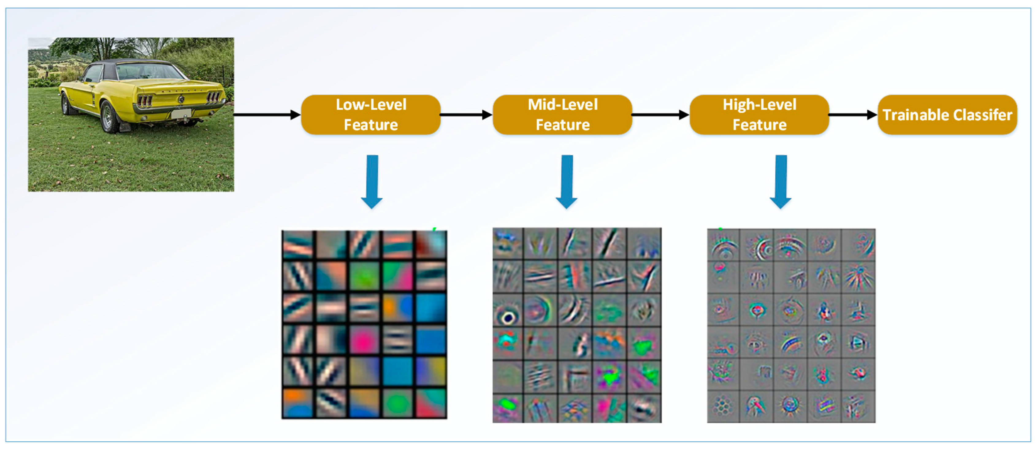
Figure 2.
3D schematic diagram of Gabor filter.

Figure 3.
Convolution kernel of two dimensional Gabor filters with various shapes.

Figure 4.
Three-dimensional color Gabor filter convolution kernel.

Figure 5.
Intelligent screening process for optimal Gabor convolution kernel set.

Figure 6.
Network Architecture of Dynamic Region Enlargement Algorithm.

Figure 7.
R-Net network framework.

Figure 8.
Dynamic zoom area selection process.

Figure 9.
Mobile video object detection framework based on time-aware feature mapping.

Figure 10.
Schematic diagram of the model processing video input and output.

Figure 11.
Overall framework of the improved detection algorithm.

Figure 12.
Small sample tuning parameters flow chart.

Figure 13.
R-net amplification precision gain effect.

Figure 14.
M5 model test results example.


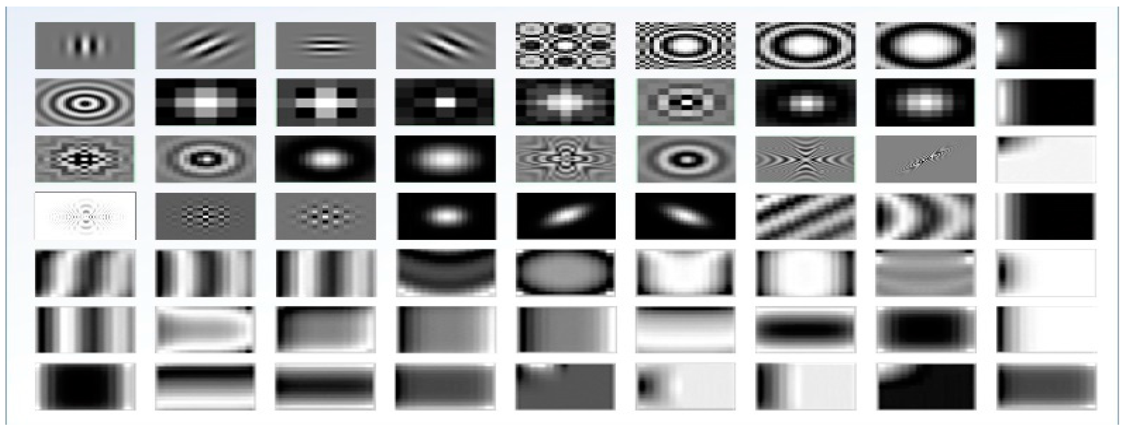
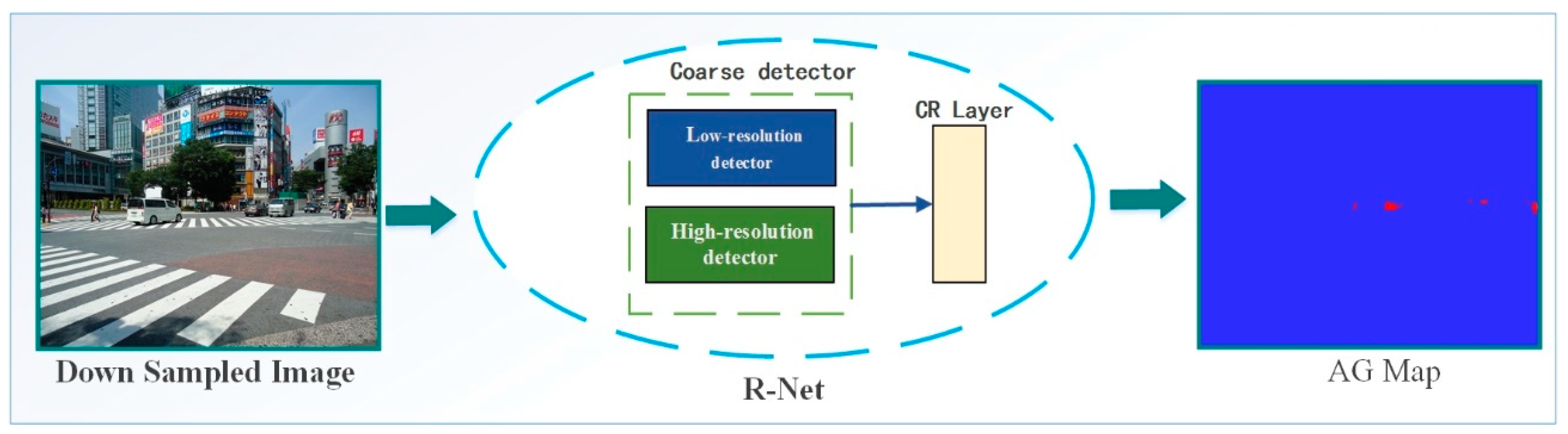
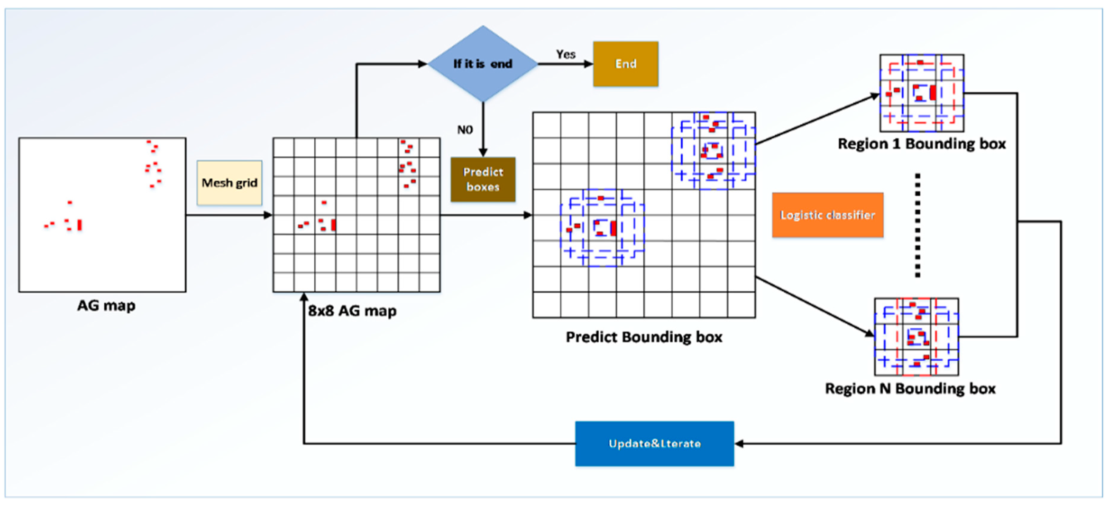
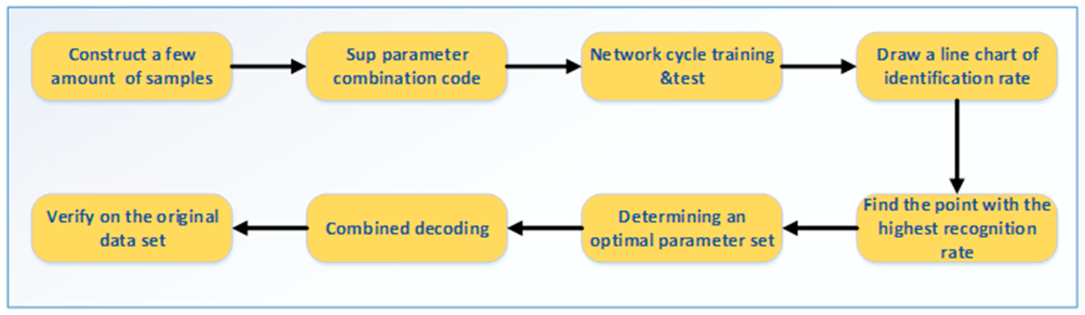
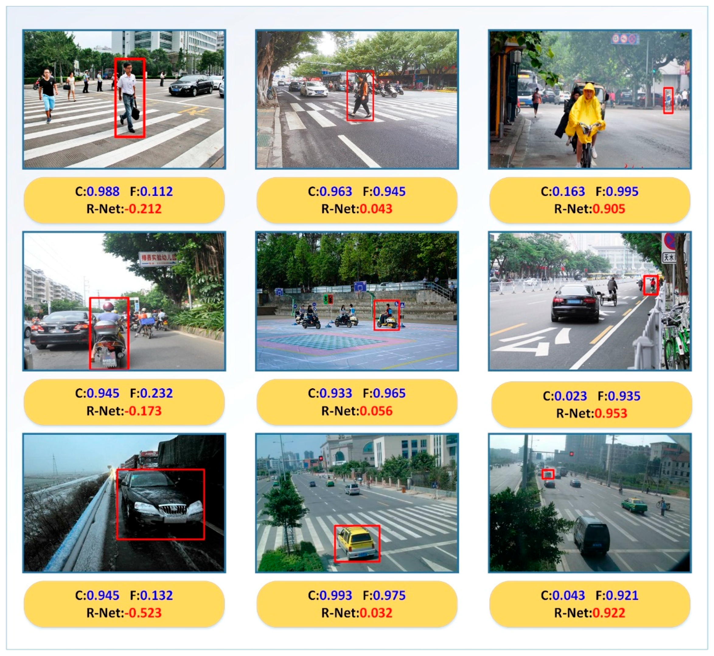
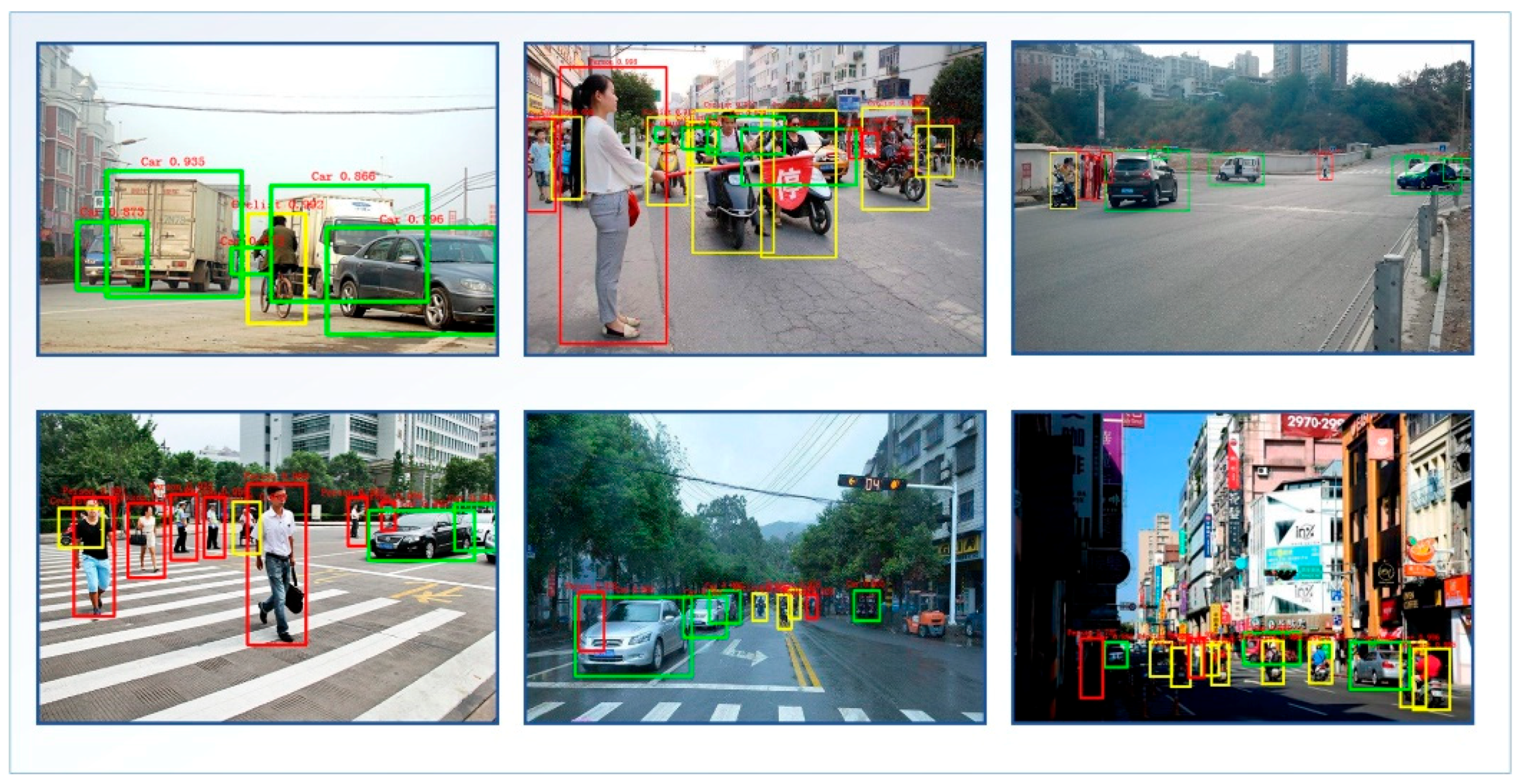
Table 1.
Comparison of each model identification and detection effect.
| Model | Dataset | AP (%) | mAP (%) | Pf (%) | Pm (%) | Pd (%) | Pe (%) | ||
|---|---|---|---|---|---|---|---|---|---|
| Person | Car | Cyclist | |||||||
| M0 | KITTI | 73.36 | 71.53 | 65.32 | 70.07 | 20.21 | 19.34 | 41.32 | 19.13 |
| WD | 71.59 | 69.63 | 62.75 | 67.99 | 19.25 | 21.38 | 38.83 | 20.54 | |
| M1 | KITTI | 87.53 | 82.16 | 78.28 | 82.66 | 16.48 | 17.91 | 57.38 | 8.23 |
| WD | 85.64 | 80.59 | 74.34 | 80.19 | 18.95 | 19.28 | 51.42 | 10.35 | |
| M2 | KITTI | 77.18 | 72.35 | 68.69 | 72.74 | 12.31 | 13.29 | 57.84 | 16.56 |
| WD | 73.52 | 70.45 | 64.83 | 69.61 | 15.17 | 14.49 | 52.45 | 17.89 | |
| M4 | KITTI | 88.42 | 81.73 | 74.38 | 81.51 | 9.53 | 11.69 | 64.25 | 14.53 |
| WD | 74.92 | 72.34 | 65.63 | 70.96 | 16.24 | 15.19 | 51.16 | 17.41 | |
| M5 | KITTI | 92.42 | 92.23 | 90.85 | 91.83 | 5.19 | 7.13 | 81.47 | 6.21 |
| WD | 88.46 | 87.38 | 83.24 | 86.36 | 8.26 | 11.27 | 71.05 | 9.42 | |
Table 2.
M4 anti-occlusion interference verification.
| Model | Evaluation Metric | Pz = 0.25 | Pz = 0.5 | Pz = 0.75 | Pz = 0.1 |
|---|---|---|---|---|---|
| M0 | mAP (%) | 53.36 | 41.24 | 22.15 | 12.89 |
| Pd (%) | 33.58 | 21.56 | 12.33 | 4.25 | |
| M4 | mAP (%) | 74.28 | 66.82 | 59.79 | 51.58 |
| Pd (%) | 60.35 | 55.62 | 51.16 | 42.39 |
Table 3.
Low-resolution small object detection effect verification.
| Model | Dataset | AP (%) | mAP (%) | Pf (%) | Pm (%) | Pd (%) | Pe (%) | ||
|---|---|---|---|---|---|---|---|---|---|
| Person | Car | Cyclist | |||||||
| M0 | KITTI | 13.63 | 19.38 | 9.73 | 14.25 | 33.12 | 29.43 | 10.14 | 27.31 |
| WD | 8.59 | 16.33 | 8.53 | 11.15 | 34.15 | 30.48 | 6.45 | 28.92 | |
| M3 | KITTI | 77.45 | 80.19 | 58.68 | 72.11 | 10.82 | 10.17 | 60.48 | 18.53 |
| WD | 65.62 | 70.49 | 52.37 | 62.83 | 11.91 | 14.85 | 52.03 | 21.21 | |
Table 4.
Comparison of detection and recognition effects of other algorithms.
| Method | Dataset | AP (%) | mAP (%) | Pd (%) | FPS | ||
|---|---|---|---|---|---|---|---|
| Person | Car | Cyclist | |||||
| Faster R-CNN | KITTI | 83.26 | 74.13 | 75.42 | 77.61 | 45.22 | 13.15 |
| WD | 81.49 | 71.33 | 68.65 | 73.82 | 36.63 | 11.64 | |
| DSOD300 | KITTI | 77.43 | 72.26 | 68.38 | 72.69 | 58.68 | 58.23 |
| WD | 70.73 | 69.39 | 67.04 | 69.05 | 52.32 | 50.35 | |
| DSSD513 | KITTI | 75.46 | 69.53 | 68.34 | 71.11 | 59.42 | 46.34 |
| WD | 72.19 | 68.83 | 66.45 | 69.16 | 49.79 | 39.38 | |
| YOLOv2 544 | KITTI | 79.43 | 71.25 | 67.32 | 72.66 | 60.82 | 56.74 |
| WD | 73.29 | 69.63 | 68.85 | 70.59 | 54.86 | 49.28 | |
| M5 | KITTI | 92.42 | 92.23 | 90.85 | 91.83 | 81.47 | 31.86 |
| WD | 88.46 | 87.38 | 83.24 | 86.36 | 71.05 | 19.83 | |
© 2018 by the authors. Licensee MDPI, Basel, Switzerland. This article is an open access article distributed under the terms and conditions of the Creative Commons Attribution (CC BY) license (http://creativecommons.org/licenses/by/4.0/).
Share and Cite
MDPI and ACS Style
Wang, X.; Hua, X.; Xiao, F.; Li, Y.; Hu, X.; Sun, P. Multi-Object Detection in Traffic Scenes Based on Improved SSD. Electronics 2018, 7, 302. https://doi.org/10.3390/electronics7110302
AMA Style
Wang X, Hua X, Xiao F, Li Y, Hu X, Sun P. Multi-Object Detection in Traffic Scenes Based on Improved SSD. Electronics. 2018; 7(11):302. https://doi.org/10.3390/electronics7110302
Chicago/Turabian StyleWang, Xinqing, Xia Hua, Feng Xiao, Yuyang Li, Xiaodong Hu, and Pengyu Sun. 2018. "Multi-Object Detection in Traffic Scenes Based on Improved SSD" Electronics 7, no. 11: 302. https://doi.org/10.3390/electronics7110302
Note that from the first issue of 2016, this journal uses article numbers instead of page numbers. See further details here.