Real-Time Road Lane Detection in Urban Areas Using LiDAR Data


1
Department of Software Convergence, Kyung Hee University, Yongin 17104, Korea
2
Department of Computer Science and Engineering, Kyung Hee University, Yongin 17104, Korea
*
Author to whom correspondence should be addressed.
Electronics 2018, 7(11), 276; https://doi.org/10.3390/electronics7110276
Submission received: 6 September 2018
/
Revised: 14 October 2018
/
Accepted: 24 October 2018
/
Published: 26 October 2018
(This article belongs to the Special Issue Machine Learning and Embedded Computing in Advanced Driver Assistance Systems (ADAS))
Abstract
:The generation of digital maps with lane-level resolution is rapidly becoming a necessity, as semi- or fully-autonomous driving vehicles are now commercially available. In this paper, we present a practical real-time working prototype for road lane detection using LiDAR data, which can be further extended to automatic lane-level map generation. Conventional lane detection methods are limited to simple road conditions and are not suitable for complex urban roads with various road signs on the ground. Given a 3D point cloud scanned by a 3D LiDAR sensor, we categorized the points of the drivable region and distinguished the points of the road signs on the ground. Then, we developed an expectation-maximization method to detect parallel lines and update the 3D line parameters in real time, as the probe vehicle equipped with the LiDAR sensor moved forward. The detected and recorded line parameters were integrated to build a lane-level digital map with the help of a GPS/INS sensor. The proposed system was tested to generate accurate lane-level maps of two complex urban routes. The experimental results showed that the proposed system was fast and practical in terms of effectively detecting road lines and generating lane-level maps.
1. Introduction
Autonomous driving vehicles with various levels of automation from semi-autonomous driving technologies such as adaptive cruise control (ACC) and lane-keeping assist systems (LKAS) to fully-autonomous driving vehicles are now commercially available on the market. While conventional digital maps for car navigation are made for human drivers and have road-level resolution, map providers are now focusing on generating digital maps with a relatively high resolution. The presence of lane-level digital maps reduces the burden of capacity and eventually the cost of each autonomous driving vehicle.
Using conventional digital maps with road-level resolution, an individual autonomous driving vehicle carries excessive burden to fully understand its surroundings to make a decision. For example, if the vehicle has to turn right at the next junction, it needs to figure out the total number of lanes on the road and the lane that the vehicle is currently in in order to move to the rightmost lane safely before reaching the junction. However, if a lane-level map were provided to the vehicle, the path planning process would become considerably simpler and safer so that the individual vehicle would be less obligated to be equipped with very expensive sensors and processors.
Unlike the road-level digital map generation process, a large part of which is automated, the process of generating a lane-level digital map usually requires manual work at many stages. Lane detection on an urban road is more difficult because of multiple lanes, diverse road signs on the ground and complex lane variations at the junctions.
In the case of road-level map generation, it is important to reflect the direction and the curvature of the road accurately, as well as the existence of ramps and overpasses. Lane-level map generation requires more details; therefore, the individual lanes must be correctly acquired via accurate road line detection followed by appropriate parameterization. If the road is simple and has only a couple of lanes with no road signs on the ground other than the road lines, the generation of a road-level map and a lane-level map will not be very different. However, a complex boulevard in an urban area has multiple lanes and various road signs mixed with road lines. In this case, fast and accurate road line detection becomes an important issue in lane-level map generation.
Many of the conventional road line detection methods using LiDAR data about a decade ago focused on detecting only two lines on each side of the vehicle, in order to reduce the unintended lane departures of an autonomous driving vehicle [1,2]. Kammel and Pitzer [3] proposed a LiDAR-based lane marker detection method, but the purpose of the algorithm was the robust estimation and correction of an offset between the provided map and the real lane on which the autonomous vehicle was traveling. As the road was rather simple, lane markers were assumed to be either the painted road lines or the curbs with some height. Jordan et al. [4] compared LiDAR-based and camera-based lane detection methods and summarized that the LiDAR-based methods detect an increase in the reflectivity of the lane markings when compared to the road surface reflectivity.
More recently, Hata and Wolf [5] detected road markings and curbs by using a 32-channel LiDAR, but the method was tested on a simple two-lane ring track, while road markings other than lines were not distinguished because the purpose of the algorithm was the localization of the vehicle. Yan et al. [6] proposed a mobile mapping system using LiDAR. All road markings including the road lines were precisely extracted to generate a high-definition point-cloud map; however, the markings were not categorized, and the lines were not parameterized for use as a lane-level digital map.
In this paper, we present a practical real-time working prototype for road lane detection in an urban area using LiDAR data. The proposed method is a fully-automated process to detect road lanes on complex urban roads with multiple lanes and diverse road signs on the ground such as arrows with different directions and stop signs. The following are the main contributions of this paper:
- Multiple lanes are detected simultaneously including the lane on which the vehicle is currently.
- Road lines are distinguished from other road markings on complex urban roads.
- Road lines are represented as uniformly-distributed 3D points to be easily used for further applications, such as road curvature calculation and lane-level map generation.
- Lane-level digital map generation by accumulating the detected road lanes is presented as an application of the proposed method.
2. Related Work
Several methods for road map generation have been developed thus far. One of the traditional methods is to use satellite images or aerial images [7,8,9]. One satellite/aerial image can cover a large area, and the road map can be generated automatically by using adequate image processing. However, up-to-date satellite images are not always available to the general public, and aerial images are expensive to update. Even though the camera resolution is rapidly increasing, it is still too limited to facilitate the generation of a lane-level map from satellite/aerial images. Moreover, as the images are two-dimensional, it is not possible to build a 3D map out of satellite/aerial images.
To build a road map without access to the satellite data or an airplane, in many studies, researchers have installed a GPS sensor on a probe vehicle and recorded its positioning information as the vehicle moves on the road [10,11,12,13,14]. This is an intuitive method of building a road map, and the accuracy of the resulting road map will depend on the accuracy of the GPS sensor. In contrast, as the GPS sensor records only the position of the vehicle, the vehicle has to pass multiple lanes one by one to generate a lane-level map. The generation of a lane-level map for a route takes a considerable amount of time and effort if the route contains many lanes. Moreover, it is difficult for a human driver to drive the vehicle on the exact center of the lane as the GPS sensor records its positions.
To resolve these shortcomings, map providers nowadays install various perception sensors on the map-making vehicles. The most popular sensor is a camera [15,16]. The use of cameras can provide the information of multiple lanes from a single frontal or an all-around view of the vehicle. The vehicle is no longer forced to be driven on the center of the lane if the GPS sensor and the cameras are calibrated. A 2D or a 3D LiDAR sensor provides the 3D information of its surroundings in real time. Although 3D information can be obtained using multiple cameras, the use of a 3D LiDAR sensor is increasing with a significant decrease in the cost of the sensor [16,17,18,19,20].
After processing the acquired data, various methods can be used to represent the generated lane-level road maps. Several researchers have studied how to represent road maps efficiently while maintaining their high usability in practical applications such as autonomous driving. Several studies have been conducted on the representation of a lane-level road map using polygons [21,22,23,24], clothoids [14,25], splines [26,27,28,29] and piecewise polynomials [30].
Instead of a particular representation, we simply represent the detected lines by using densely- and uniformly-distributed 3D points along the detected road lines. As lane-level maps used for autonomous driving do not have a global standard to represent the road lines, there are pros and cons to choosing any of the representations mentioned above, and it is inevitable to need to transform a certain representation to another to calculate road characteristics such as the curvature or the tangent of the road. Therefore, because of the computational advantage with little burden for storage, we represent the detected road lines using densely- and uniformly-distributed 3D points along the line, which can easily be processed to any other representations for further application.
Finally, it is worth mentioning a few more studies on road detection using LiDAR in recent years. Clode et al. [31] presented a method for automatic road detection from airborne laser scanner (ALS) data. The test data were collected from Fairfield in Sydney, Australia, with an approximate point density of one point per in the area of 2 km × 2 km. The method classified road or non-road using height and intensity information of ALS data. Later, Clode et al. [32] proposed a more mature method for road/non-road classification using the same dataset, including road vectorization with appropriate parameters such as centerline, orientation and width.
Zhang [33] presented road and road edge (curb) detection method using a 2D LiDAR sensor, which was demonstrated in a prototype vehicle in the DARPA Urban Challenge 2007. A forward down-looking 2D LiDAR sensor was equipped on the front-top of the vehicle, and the elevation information of the range data was used to detect the lowest smooth surface as the drivable region and curbs as road edges. Han et al. [34] presented a road boundary and obstacle detection method for the 2010 Autonomous Vehicle Competition in Korea using a downward-looking 2D LiDAR. The method detected drivable region and obstacles on the road boundary such as curbs, bushes, traffic cones and vehicles. Both methods [33,34] were successfully demonstrated through competition participation; however, the road condition in the test fields was limited to two lanes, and the road lanes were not detected. Yuan et al. [35] presented a road detection and corner extraction method using a 3D LiDAR for robot navigation on the pavement. The test fields were narrow sidewalks surrounded by bushes or buildings, which were distinguished by corner extraction from range data.
Fernandes et al. [36] proposed a road detection method using 3D LiDAR data. The authors projected 3D LiDAR points on a 2D reference image plane and upsampled the points to generate dense height maps. The method detected road surface, which is the drivable region, from the dense height maps surrounded by road boundaries with elevation such as curbs or parked vehicles. Caltagirone et al. [37] proposed a 3D LiDAR-based road detection method using fully-convolutional neural networks (FCN). The FCN was designed for a pixel-wise semantic segmentation task in the point cloud top-view images. The proposed system carried out road segmentation in real time. While both methods [36,37] were successfully tested using the KITTI road benchmark [38], only the drivable region was detected, and road lanes were not distinguished.
3. Proposed System
The proposed method detects the drivable region and road lines from LiDAR data in stages. The LiDAR data are assumed to be scanned from a spinning multi-channel LiDAR sensor installed on top of a vehicle while driving on the urban road.
3.1. Overview
A spinning multi-channel LiDAR sensor spins 5–20 times in a second to densely scan its surroundings with the same number of scanlines as the number of channels. Usually, it scans up to 100 m, which is sufficiently far for a moving vehicle to detect any object in advance and take appropriate action in time. However, a sensor with less than 16 channels may have limited vertical resolution to recognize an object located more than 30 m away.
As we aimed to detect road lines on the ground rather than vertical obstacles by using LiDAR data, we were less obligated to process LiDAR points far away from the sensor. Therefore, it was reasonable to exclude the LiDAR points scanned far away from the sensor with limited resolution. The proposed strategy processed the LiDAR points inside a certain perimeter with an appropriate vertical resolution to be accurately categorized. The detected road lines were later accumulated with the help of a GPS/INS sensor for digital map generation.
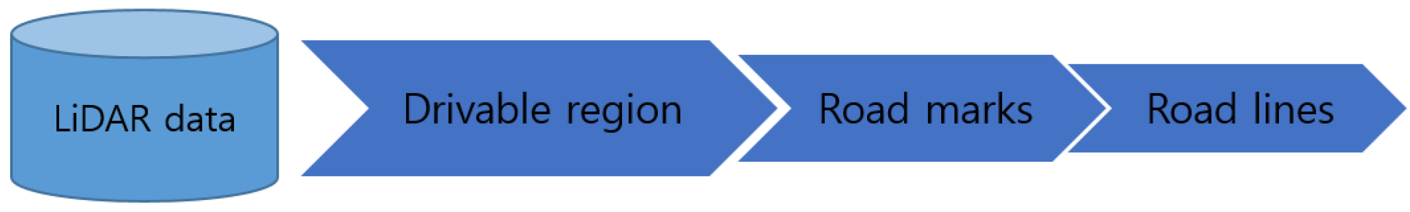
We processed the three stages of LiDAR point categorization for road lane detection as illustrated in Figure 1. First, we differentiated the LiDAR points of the drivable region on the ground from the points scanned inside a certain perimeter from the sensor. We assumed that the vehicle was currently on the road and examined the vertical slope between the LiDAR points of the adjacent channels in the radial direction. If the slope was smaller than a certain threshold, the point was categorized as the drivable region until an obstacle was faced. Then, among the points categorized as the drivable region, we distinguished the points of road marks by their intensity. A LiDAR point carried an intensity value, as well as its 3D location, which depended on the reflexibility of the scanned surface. The paint used for the road marks usually had higher reflexibility than the asphalt or cement on the road. Therefore, the points of the road marks could easily be categorized from the points of the drivable region by using the intensity.
The final stage of distinguishing road lines from the points categorized as road marks was a difficult problem. Previous works circumvented the issue by detecting the road lines of the simple roads having at most two lanes with few road signs on the ground. In this case, road line detection became as simple as categorizing the LiDAR points with a high intensity from the points of the drivable region. However, diverse road marks such as arrows, stop signs and the names of different destinations of individual lanes frequently appeared on the urban roads. It was difficult to distinguish them from the road lines because road marks and road lines usually had the same reflexibility to the LiDAR scan.
3.2. LiDAR Point Categorization
A multi-channel LiDAR sensor carries multiple laser scanners, as many as the number of its channels. They are usually installed vertically inside the sensor. Each laser scanner emits and receives light to measure the distance for each channel. In order to scan the entire surroundings of the sensor, a mirror inside the sensor spins rapidly to scan 360.
We categorized the LiDAR points inside a certain perimeter from the sensor as the drivable region by calculating the slope between the points in the radial direction from the sensor. When a spinning multi-channel LiDAR horizontally scanned 360 with multiple laser emitters vertically installed on the sensor, the points of multiple channels scanned at the same instance formed a ray from the sensor. For example, Velodyne HDL-32E horizontally scanned 360 in 0.1 s with 32 lasers. Each channel scanned approximately 2100 points per spin; therefore, approximately six points were densely positioned in each degree angle. Furthermore, 32 points scanned at the same time formed a ray from the sensor. If we considered the point nearest to the sensor as Channel Number 0 and the the point furthest from the sensor as Channel Number 31, we could calculate the slope between two points of the adjacent channels from Channels 0–31 as follows:
where a and b indicate the adjacent channels and x, y and z indicate the 3D coordinates of each LiDAR point in the right, forward and up directions from the sensor, respectively. When the slope s of the ground became greater than a certain threshold (i.e., we empirically set the value to 0.15), we assumed that there was a vertical obstacle on the ground and categorized the points on the same ray beyond this channel as not drivable.
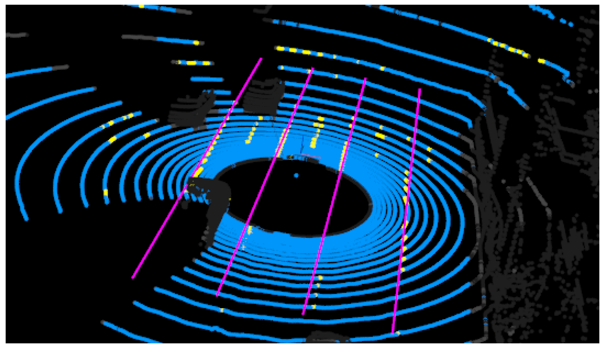
This method effectively detected sudden vertical slope changes on the road such as the curb between the road and the sidewalk or vertical obstacles such as the median strip, beacons or other vehicles. The method successfully categorized speed bumps or small potholes as the drivable regions. An example of drivable region detection is shown in Figure 2. Gray points indicate the given 3D LiDAR points, whereas blue points indicate the points categorized as the drivable region.
Once the points of the drivable region were discriminated, we distinguished the points of road marks by using the LiDAR point intensity. The signs and lines on the road were usually painted with conspicuous colors such as white or yellow. The intensity of the points scanned at the road marks was easily distinguishable from the intensity of the points scanned at the asphalt or cement on the ground. The LiDAR point intensity of the road marks was usually considerably higher. In Figure 2, the yellow points indicate the detected road marks on the ground.
3.3. Road Line Detection
To detect the road lines out of various road marks having similar LiDAR intensities, we searched for a set of parallel lines separated by the interval of the lane width. The lane width was initially set as 3.4 m, but the value was updated during the detection process.
Given a set of LiDAR points categorized as road marks, we aimed to estimate L sets of line parameters. We modeled each road line in 3D as:
where is a vector parallel to the line, is a point on the line and t is a real number.
For initialization, we initialized sets of lines with the interval of half of the initial lane width to separate the road marks from the road lines effectively, where K is the number of candidates to detect L lines. Assuming that the location of the sensor was the origin and the sensor was facing front, all the line parameters were initialized as follows:
This initialization indicates that all the lines are parallel to the y-axis and lie on the ground two meters below the sensor. Note that the and z axes point in the right, forward and up directions, respectively. The values for the lines were initialized to be separated with intervals of w, where w is the initial lane width set as .
After initialization, we updated the value of each line with the assumption that the LiDAR points for the line were stably found when the vehicle moved forward, whereas the points for the other road marks were discontinued. We designed an iterative expectation-maximization (EM) algorithm to determine reliable sets of line parameters. For each iteration, we assigned each LiDAR point to its nearest line by calculating the point-line distance. After the assignment, we updated for each line to be the average of the x-coordinate values of the assigned points. This process was very simple and fast. We repeated the process 100 times for each spin of the LiDAR.
Finally, we selected L reliable sets of line parameters out of the updated sets after the EM-algorithm. For each line k, we calculated the number of assigned points for each line and the standard deviation of the y-coordinate values of the assigned points. showed the level of distribution of the points in the direction of the y-axis. of the cluster of a line tended to be larger than that of the cluster of other road marks. From the cluster having the largest , we selected the line parameters as a reliable set if was larger than a certain threshold. As the line was expected to be continued from the last spin, we also checked if the current line was continued from one of the detected lines from the last spin. That is, we calculated the minimum difference between with the values of the detected lines from the last spin and considered it as the same line when the minimum difference was below a certain threshold. After selecting L sets of reliable line parameters, we ended the line selection process.
As a result, the detected L sets of line parameters were updated at every spin of the LiDAR. The lines were stably detected, while the vehicle changed lanes or went through curved roads. Algorithm 1 summarizes the proposed road line detection process.
3.4. Lane-Level Digital Map Generation
Nowadays, most of the map-making cars are equipped with a GPS/INS sensor, which provides the current GPS location of the vehicle, as well as the rotation matrix from the sensor coordinate to the world coordinate. The world coordinate generally refers to the north-east-down (NED) coordinate. Provided that the GPS/INS sensor was calibrated with the LiDAR sensor, we transferred the estimated parameter of the detected road lines to the world coordinates for each spin of the LiDAR.
We used the current position in terms of the latitude and longitude along with the altitude provided by the GPS/INS sensor, as well as the rotation matrix that transformed the sensor coordinate frame to the local NED coordinate in real time. No additional method was used to post-process the positioning data. The latitude and longitude values were converted to the UTM coordinate to obtain the position values in meters. As the estimated parameter was the x-coordinate value in the sensor coordinate frame, it was transformed to a position in the world coordinates by multiplying the rotation matrix and then adding the current sensor position in UTM.
| Algorithm 1: Road line detection. |
 |
We filtered out the duplicate dots, which were estimated while the vehicle stopped or moved very slowly. Then, we simply connected the dots to build the lane-level digital map. For qualitative evaluation, we overlapped the final lane-level digital map with the satellite images.
4. Results
4.1. Data Acquisition
The data to evaluate the proposed road lane detection method were collected using a vehicle equipped with a 32-channel 3D LiDAR (Velodyne HDR-32E). For the lane-level map generation, we used a GPS/INS sensor (Ekinox-D). Velodyne HDR-32E has 32 laser scanners with a horizontal field-of-view of 360 a vertical field-of-view of 40 and an angular resolution of 1.33. We set the rotation rate to be 10 Hz and gathered approximately 69,000 points per spin in 0.1 s. Ekinox-D is an inertial navigation system with an integrated dual antenna GNSS receiver that provides highly accurate 6D vehicle poses. It combines an inertial measurement unit (IMU) and runs an enhanced on-board extended Kalman filter (EKF) to fuse real-time inertial data with internal GNSS information. The sensor embeds a GNSS receiver, capable of centimeter-scale accuracy by using an RTK solution [39,40]. The vehicle was driven at a normal speed, from 0–60 km/h, depending on the traffic situation. All experiments were carried out on a PC with a 3.40-GHz i7-6800K CPU.
The dataset was collected along two different routes in the cities of Seongnam and Incheon, South Korea, which are the 10th and the third largest cities in the country with a population of nearly one million and three million, respectively. Route 1 is an expressway with sidewalks in the city of Seongnam. It is approximately 7 km in round trip and contains junctions, crosswalks, ramps and a tunnel. The number of lanes changes from one to three on one side of the road. Because of a wide separation area at the center of the road, we only processed one side of the road of the current driving direction first and then processed the other side on the way back. Route 2 travels along the major boulevard in the city of Incheon with a length of approximately 2 km in round trip. The route contains junctions, crosswalks and various road marks on the ground.
4.2. Qualitative Results
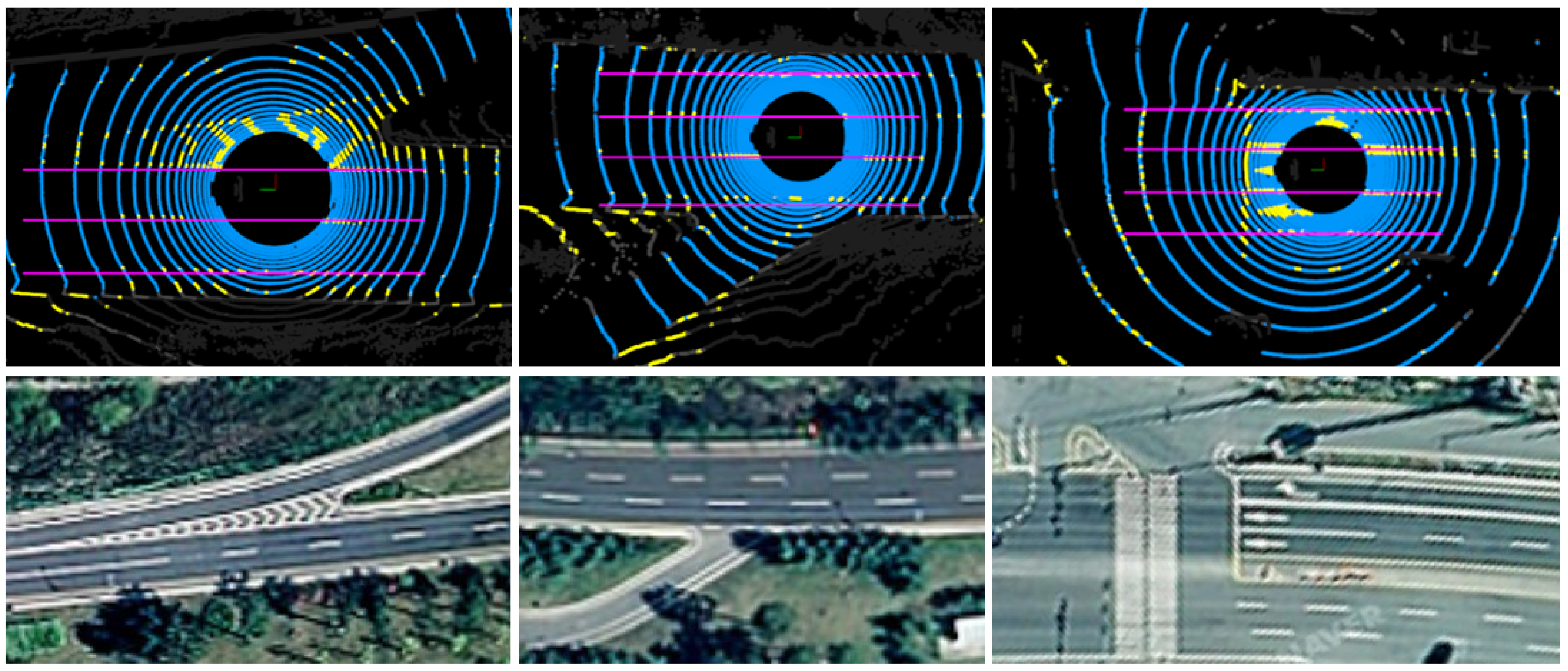
Both Route 1 and Route 2 were modeled using densely- and uniformly-distributed 3D points on the road lines. Figure 3 shows three different examples of drivable region categorization and road line detection with two or three lanes on the road in the presence of ramps or junctions. Gray points indicate the given 3D point cloud scanned by a 3D LiDAR; blue points indicate the drivable region; yellow points indicate the road marks on the ground; and magenta lines are the final results of the road line detection at each spin of the LiDAR sensor.
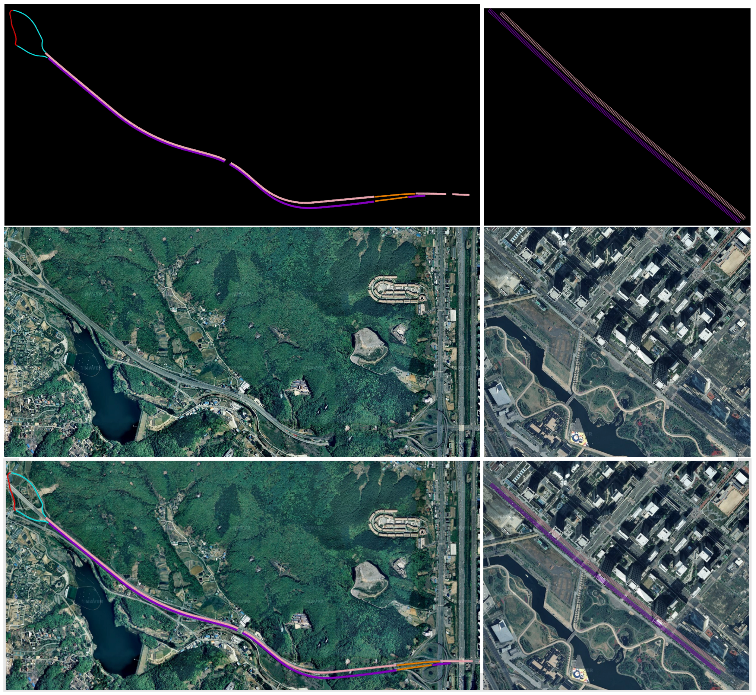
The detected road line was parameterized, and its parameters were recorded as a 3D point on the line in the NED coordinate with the help of a GPS/INS sensor. Figure 4 shows the result of the 3D lane-level map of Route 1 and Route 2 generated by connecting these 3D points, as well as the corresponding satellite images for a reference. In Figure 4, pink and magenta lines indicate three-lane regions in opposite directions. Orange lines indicate two-lane regions, and cyan lines indicate one-lane regions where the vehicle was driving on the ramp to get off or to get on the main driveway. The red line is an off-road region with no official road line on the ground. We added the red line manually just to show the entire route. The disconnected parts indicate junctions with crosswalks and stop lines. As the road lines were disconnected at the junctions, the resulting map lines were disconnected, as well.
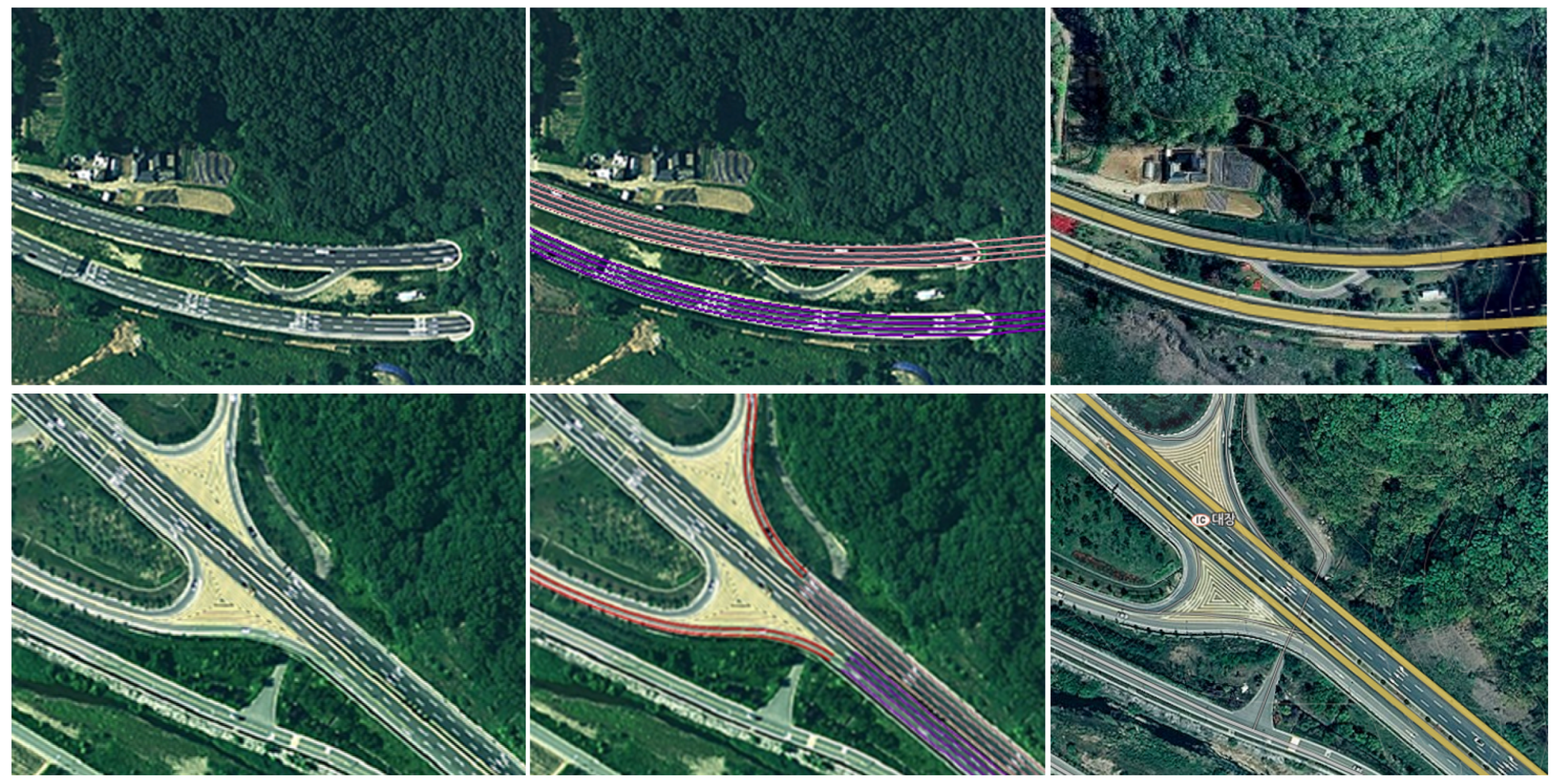
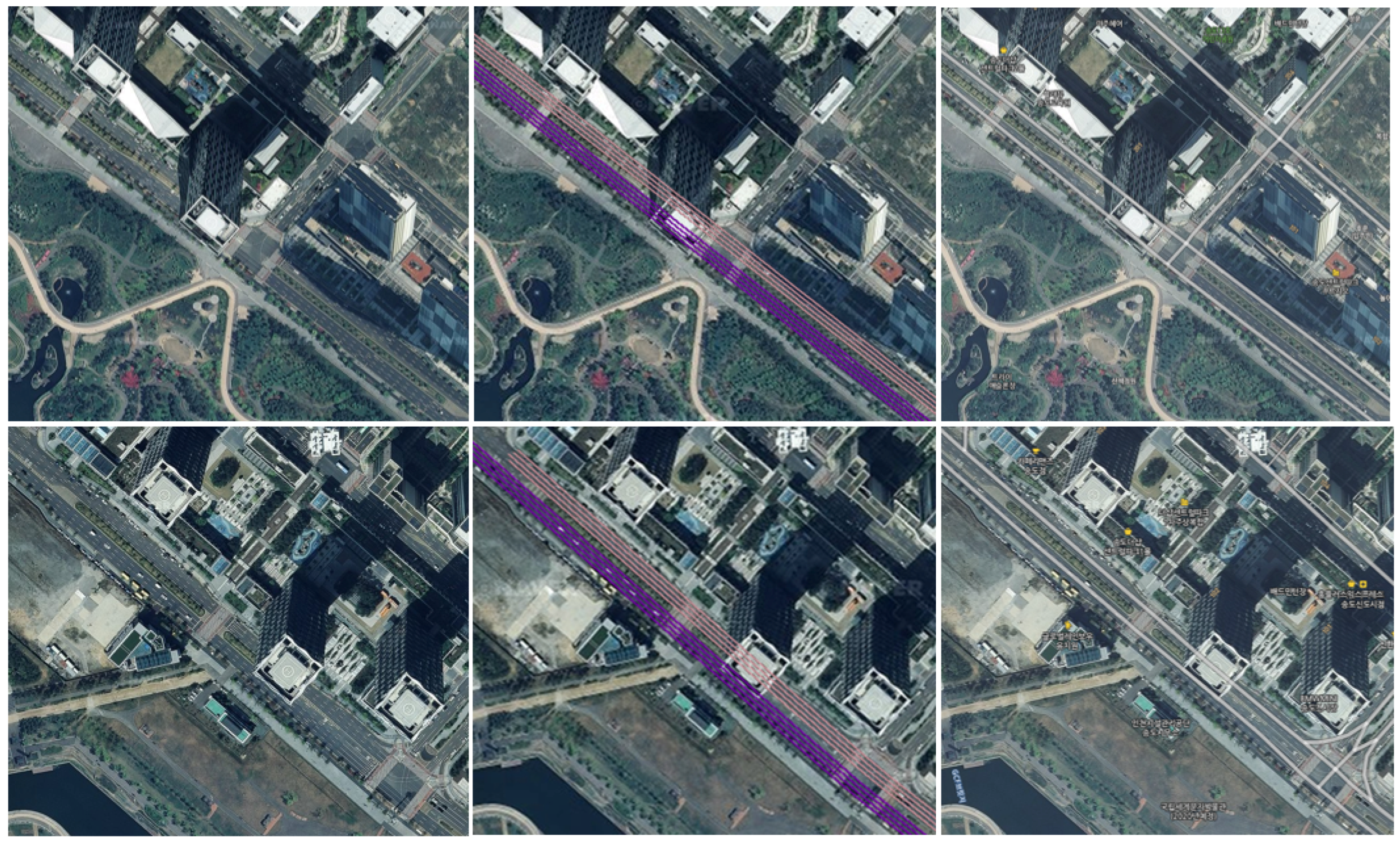
As it was difficult to evaluate the accuracy of the generated lane-level map quantitatively, we overlaid the resulting lane-level map on the satellite image provided by Naver Map [41] for the qualitative evaluation. Figure 5 and Figure 6 show the lane-level maps overlapped with the corresponding satellite images of Route 1 and Route 2 in magnified views, respectively. The left column shows the satellite images, the middle column the resulting lane-level map overlapped with the satellite images and the right column the existing road-level map provided by Naver Map [41]. We observed that the detected road lanes of the generated map were accurately synchronized with the road lanes in the satellite images.
A comparison of the overall routes and the corresponding satellite images in Figure 4 revealed that the lanes were accurately detected and well represented by connecting the 3D points obtained from the line parameters. Although Route 2 was short and looked simple, it was a challenging route with heavy traffic and complex road signs on the ground. Moreover, many tall buildings interrupted the GPS signals and made it more difficult to generate a lane-level map without the use of perception sensors. Note that the resulting lanes were accurately overlapped with the road lines in the satellite images, whereas the existing road-level map roughly represented the wide road in the macroscale, as shown in Figure 6.
In order to evaluate the consistency of the detected road lines with the existing road-level map, we extracted the middle line from the road-level map provided by Naver Map [41] and calculated the point-line distance from our final 3D point representation of the detected road lines. As our representation existed for multiple lanes and a road-level map provided only one line, the mean distance varied for each line, but the standard deviation remained small, which showed that our result was consistent with the road-level map. The standard deviation for Route 1 was relatively large because the middle line extracted from the road-level map of Route 1 fluctuated from Line 2 to Line 3. Route 2 was rather straight, so the middle line of the road-level map of Route 2 was relatively consistent near Line 3 (towards the northwest) and between Line 2 and Line 3 (towards the southeast). Therefore, the standard deviation remained very small, less than 10 cm. Note that as the reference (road-level map) did not provide the ground-truth road line position, Table 1 does not show the absolute performance of the proposed method, but provides some clues of the consistency of our road line detection results with the existing road-level map.
5. Discussion and Conclusions
5.1. Limitations and Future Work
There are several limitations to our system, which need to be addressed before a full solution for the given issue can be developed. The proposed method aimed for lane-level map generation by using the detected road lines rather than immediate lane keeping during autonomous driving as an application. Therefore, we did not consider heavy weather conditions, which might degrade the 3D LiDAR sensor input. When the purpose was mapping, we could simply choose a good weather day to scan the road, whereas this can be a critical limitation when the method is applied for road lane detection for a lane keeping system. When used for lane keeping in bad weather, the proposed method might be simplified to detect only two road lines on each side of the current vehicle, and the input data could be compensated by other perception sensors, such as cameras.
While it is one of the strengths that the proposed method was tested on complex urban roads, this can also indicate that the method was difficult to apply to unpaved roads. Roads with drastic slopes and severe curvatures in mountainous areas could be challenging and might require some different empirical threshold values for the proposed method.
Finally, while vehicles crossing road lines as they changed lanes during driving were never a critical problem for the proposed algorithm, it was difficult to detect the road lines beneath the parked cars on the side, completely obscuring the road lines. As the undetected road line was usually the rightmost line in this case, this issue could be alleviated by knowing the total number of lines to be detected beforehand. If we have prior knowledge that there should be another line to be detected, we can adjust the algorithm to detect the rightmost line using less input data observed between the parked cars.
Potential future work would depend on a further application of the proposed road lane detection method. For example, if we aim to extend the proposed method for use in a lane-keeping assist system for autonomous driving vehicles, we should focus on improving the detection accuracy of the two lines on each side of the vehicle under various weather and lighting conditions. To extend the proposed method toward fully-automated lane-level map generation, we should test the method under various road conditions, such as unpaved roads, mountainous roads with severe slope and curvature, crowded urban roads and roads with noisy GPS signals.
5.2. Conclusions
In this paper, we presented a simple and practical real-time working prototype for road lane detection in an urban area by using 3D LiDAR points. The overall system consisted of two subsystems, including point categorization and road line detection. Given the 3D LiDAR point cloud, we categorized the points of the drivable region and distinguished the points of the road signs on the ground. Then, we presented an expectation-maximization process to detect and update the 3D line parameters in real time. The detected road lines were represented as densely- and uniformly-distributed 3D points on the lines with the help of a GPS/INS sensor and integrated to generate a lane-level digital map. The proposed system was tested to generate the lane-level maps of two complex urban routes in the cities of Seongnam and Incheon, South Korea. The accuracy of the resulting lane-level map was evaluated by comparing with the corresponding satellite images.
Author Contributions
Conceptualization, J.J.; Methodology, J.J.; Software, J.J.; Validation, S.-H.B.; Writing—Original Draft, J.J.; Writing—Review & Editing, S.-H.B.
Funding
This research was funded by Kyung Hee University (KHU-20170718) and the National Research Foundation of Korea (NRF-2017R1C1B5075945).
Acknowledgments
This work was partially implemented when the first author was with Naver Labs.
Conflicts of Interest
The authors declare no conflict of interest.
Abbreviations
The following abbreviations are used in this manuscript:
| 2D | Two-dimensional |
| 3D | Three-dimensional |
| LiDAR | Light detection and ranging |
| GPS | Global positioning system |
| INS | Inertial navigation system |
| GNSS | Global navigation satellite system |
| RTK | Real-time kinematic |
| UTM | Universal Transverse Mercator |
| PC | Personal computer |
| CPU | Central processing unit |
References
- Reyher, A.; Joos, A.; Winner, H. A lidar-based approach for near range lane detection. In Proceedings of the IEEE Intelligent Vehicle Symposium, Las Vegas, NV, USA, 6–8 June 2005; pp. 147–152. [Google Scholar]
- Lindner, P.; Richter, E.; Wanielik, G.; Takagi, K.; Isogai, A. Multi-Channel Lidar Processing for Lane Detection and Estimation. In Proceedings of the 12th International IEEE Conference on Intelligent Transportation Systems, St. Louis, MO, USA, 3–7 October 2009; pp. 202–207. [Google Scholar]
- Kammel, S.; Pitzer, B. Lidar-based lane marker detection and mapping. In Proceedings of the 2008 IEEE Intelligent Vehicles Symposium, Eindhoven, The Netherlands, 4–6 June 2008; pp. 1137–1142. [Google Scholar]
- Jordan, B.; Rose, C.; Bevly, D. A Comparative Study of Lidar and Camera-based Lane Departure Warning Systems. In Proceedings of the ION GNSS 2011, Portland, OR, USA, 20–23 September 2011. [Google Scholar]
- Hata, A.; Wolf, D. Road marking detection using LIDAR reflective intensity data and its application to vehicle localization. In Proceedings of the International IEEE Conference on Intelligent Transportation Systems (ITSC), Qingdao, China, 8–11 October 2014. [Google Scholar]
- Yan, L.; Liu, H.; Tan, J.; Li, Z.; Xie, H.; Chen, C. Scan Line Based Road Marking Extraction from Mobile LiDAR Point Clouds. Sensors 2016, 16, 903. [Google Scholar] [CrossRef] [PubMed]
- Amo, M.; Martinez, F.; Torre, M. Road extraction from aerial images using a region competition algorithm. IEEE Trans. Image Process. 2006, 15, 1192–1201. [Google Scholar] [CrossRef] [PubMed]
- Hu, J.; Razdan, A.; Femiani, J.; Cui, M.; Wonka, P. Road network extraction and intersection detection from aerial images by tracking road footprints. IEEE Trans. Geosci. Remote Sens. 2007, 45, 4144–4157. [Google Scholar] [CrossRef]
- Seo, Y.-W.; Urmson, C.; Wettergreen, D. Exploiting publicly available cartographic resources for aerial image analysis. In Proceedings of the International Conference on Advances in Geographic Information Systems, Redondo Beach, CA, USA, 7–9 November 2012; pp. 109–118. [Google Scholar]
- Rogers, S. Creating and evaluating highly accurate maps with probe vehicles. In Proceedings of the IEEE Intelligent Transportation Systems, Dearborn, MI, USA, 1–3 October 2000; pp. 125–130. [Google Scholar] [Green Version]
- Qi, H.; Moore, J. Direct Kalman filtering approach for GPS/INS integration. IEEE Trans. Aerosp. Electron. Syst. 2002, 38, 687–693. [Google Scholar]
- Schroedl, S.; Wagstaff, K.; Rogers, S.; Langley, P.; Wilson, C. Mining GPS traces for map refinement. Data Min. Knowl. Discovery 2004, 9, 59–87. [Google Scholar] [CrossRef]
- Caron, F.; Duflos, E.; Pomorski, D.; Vanheeghe, P. GPS/IMU data fusion using multisensor Kalman filtering: introduction of contextual aspects. Inf. Fusion 2006, 7, 221–230. [Google Scholar] [CrossRef]
- Betaille, D.; Toledo-Moreo, R. Creating enhanced maps for lane-level vehicle navigation. IEEE Trans. Intell. Transp. Syst. 2010, 11, 786–798. [Google Scholar] [CrossRef]
- Ziegler, J.; Dang, T.; Franke, U.; Lategahn, H.; Bender, P.; Schreiber, M.; Strauss, T.; Appenrod, N.; Keller, G.G.; Kaus, E.; et al. Making Bertha Drive—An autonomous journey on a historic route. IEEE Intell. Transp. Syst. Mag. 2014, 6, 8–20. [Google Scholar] [CrossRef]
- Roh, H.; Jeong, J.; Cho, Y.; Kim, A. Accurate Mobile Urban Mapping via Digital Map-Based SLAM. Sensors 2016, 16, 1315. [Google Scholar] [CrossRef] [PubMed]
- Boyko, A.; Funkhouser, T. Extracting road from dense point clouds in large scale urban environment. ISPRS J. Photogramm. Remote Sens. 2011, 66, S2–S12. [Google Scholar] [CrossRef]
- Mancini, A.; Frontoni, E.; Zingaretti, P. Automatic road object extraction from mobile mapping systems. In Proceedings of the IEEE/ASME International Conference on Mechatronic and Embedded Systems and Applications, Suzhou, China, 8–10 July 2012; pp. 281–286. [Google Scholar]
- Guan, H.; Li, J.; Yu, Y.; Wang, C.; Chapman, N.; Yang, B. Using mobile laser scanning data for automated extraction of road markings. ISPRS J. Photogramm. Remote Sens. 2014, 87, 93–107. [Google Scholar] [CrossRef]
- Joshi, A.; James, M.R. Generation of accurate lane-level maps from coarse prior maps and lidar. IEEE Intell. Transp. Syst. Mag. 2015, 7, 19–29. [Google Scholar] [CrossRef]
- Safra, E.; Kanza, Y.; Sagiv, Y.; Doytsher, Y. Efficient integration of road maps. In Proceedings of the 14th annual ACM International Symposium on Advances in Geographic Information Systems, Arlington, VA, USA, 10–11 November 2006; pp. 59–66. [Google Scholar]
- Haklay, M.; Weber, P. OpenStreetMap: User-generated street maps. IEEE Pervasive Comput. 2008, 7, 12–18. [Google Scholar] [CrossRef]
- Vatavu, A.; Danescu, R.; Nedevschi, S. Environment perception using dynamic polylines and particle based occupancy grids. In Proceedings of the IEEE 7th International Conference on Intelligent Computer Communication and Processing, Cluj-Napoca, Romania, 25–27 August 2011; pp. 239–244. [Google Scholar]
- Sivaraman, S.; Trivedi, M.M. Dynamic probabilistic drivability maps for lane change and merge driver assistance. IEEE Trans. Intell. Transp. Syst. 2014, 15, 2063–2073. [Google Scholar] [CrossRef]
- Gikas, V.; Stratakos, J. A novel geodetic engineering method for accurate and automated road/railway centerline geometry extraction based on the bearing diagram and fractal behavior. IEEE Trans. Intell. Transp. Syst. 2012, 13, 115–126. [Google Scholar] [CrossRef]
- Schindler, A.; Maier, G.; Pangerl, S. Exploiting arc splines for digital maps. In Proceedings of the 14th International IEEE Conference on Intelligent Transportation Systems, Washington, DC, USA, 5–7 October 2011; pp. 1–6. [Google Scholar]
- Schindler, A.; Maier, G.; Janda, F. Generation of high precision digital maps using circular arc splines. In Proceedings of the IEEE Intelligent Vehicles Symposium, Alcala de Henares, Spain, 3–7 June 2012; pp. 246–251. [Google Scholar]
- Brummer, S.; Janda, F.; Maier, G.; Schindler, A. Evaluation of a mapping strategy based on smooth arc splines for different road types. In Proceedings of the 16th International IEEE Conference on Intelligent Transportation Systems, The Hague, The Netherlands, 6–9 October 2013; pp. 160–165. [Google Scholar]
- Jo, K.; Sunwoo, M. Generation of a precise roadway map for autonomous cars. IEEE Trans. Intell. Transp. Syst. 2014, 15, 925–937. [Google Scholar] [CrossRef]
- Gwon, G.-P.; Hur, W.-S.; Kim, S.-W.; Seo, S.-W. Generation of a Precise and efficient lane-level road map for intelligent vehicle systems. IEEE Trans. Veh. Technol. 2017, 66, 4517–4533. [Google Scholar] [CrossRef]
- Clode, S.; Kootsookos, P.J.; Rottensteiner, F. The automatic extraction of roads from LIDAR data. In Proceedings of the XXth ISPRS Congress Technical Commission III, Istanbul, Turkey, 12–23 July 2004; pp. 231–236. [Google Scholar]
- Clode, S.; Rottensteiner, F.; Kootsookos, P.J.; Zelniker, E. Detection and vectorization of roads from lidar data. Photogramm. Eng. Remote Sens. 2007, 73, 517–535. [Google Scholar] [CrossRef]
- Zhang, W. LIDAR-based road and road-edge detection. In Proceedings of the IEEE Intelligent Vehicles Symposium, San Diego, CA, USA, 21–24 June 2010; pp. 845–848. [Google Scholar]
- Han, J.; Kim, D.; Lee, M.; Sunwoo, M. Enhanced road boundary and obstacle detection using a downward-looking LIDAR sensor. IEEE Trans. Veh. Technol. 2012, 61, 971–985. [Google Scholar] [CrossRef]
- Yuan, X.; Zhao, C.-X.; Zhang, H.-F. Road detection and corner extraction using high definition Lidar. Inf. Technol. J. 2010, 9, 1022–1030. [Google Scholar]
- Fernandes, R.; Premebida, C.; Peixoto, P.; Wolf, D.; Nunes, U. Road detection using high resolution lidar. In Proceedings of the IEEE Vehicle Power and Propulsion Conference, Coimbra, Portugal, 27–30 October 2014. [Google Scholar]
- Caltagirone, L.; Scheidegger, S.; Svensson, L.; Wahde, M. Fast LIDAR-based road detection using fully convolutional neural networks. In Proceedings of the IEEE Intelligent Vehicles Symposium, Los Angeles, CA, USA, 11–14 June 2017; pp. 1019–1024. [Google Scholar]
- Fritsch, J.; Kuehnl, T.; Geiger, A. A new performance measure and evaluation benchmark for road detection algorithms. In Proceedings of the International Conference on Intelligent Transportation Systems, The Hague, The Netherlands, 6–9 October 2013; pp. 1693–1700. [Google Scholar]
- EKINOXUM 1.3.1 Ekinox AHRS & INS. Tactical Grade MEMS Inertial Sensors, User Manual; SBG Systems: Rueil-Malmaison, France, 2015. [Google Scholar]
- Teunissen, P.; Montenbruck, O. (Eds.) Handbook of Global Navigation Satellite Systems; Springer: Cham, Switzerland, 2017; ISBN 978-3-319-42926-7. [Google Scholar]
- Naver Map. Available online: https://map.naver.com (accessed on 1 July 2018).
Figure 1.
LiDAR point categorization.

Figure 2.
Example of LiDAR point categorization and the road line detection result. Blue points indicate the drivable region, yellow points the road marks including road lines and the magenta lines the detected road lines.
Figure 2.
Example of LiDAR point categorization and the road line detection result. Blue points indicate the drivable region, yellow points the road marks including road lines and the magenta lines the detected road lines.

Figure 3.
Three different examples of drivable region categorization and road line detection with two or three lanes on the road in the presence of ramps on the right or left (left, middle) and at the junction (right). The figures below show the satellite images of the same scene for better understanding.

Figure 4.
Result of the lane-level digital map and the corresponding satellite images of Route 1 (left) and Route 2 (right). Magnified views are provided below.
Figure 4.
Result of the lane-level digital map and the corresponding satellite images of Route 1 (left) and Route 2 (right). Magnified views are provided below.

Figure 5.
Detected road lanes on Route 1 are accumulated to build a lane-level digital map with the help of a GPS/INS sensor. The left column shows the satellite images, the middle column the resulting lane-level map overlapped with the satellite images and the right column the existing road-level map provided by Naver Map [41].

Figure 6.
More results of the detected road lanes on Route 2 are accumulated to generate a lane-level digital map with the help of a GPS/INS sensor. The left column shows the satellite images, the middle column the resulting lane-level map overlapped with the satellite images and the right column the existing road-level map provided by Naver Map [41].


Table 1.
Consistency evaluation with the commercial road-level map [41].
Table 1.
Consistency evaluation with the commercial road-level map [41].
| Route 1 | Mean (m) | St.Dev. (m) | Route 2 | Mean (m) | St.Dev. (m) |
|---|---|---|---|---|---|
| Line 1 (West) | 4.724 | 1.684 | Line 1 (Northwest) | 7.621 | 0.079 |
| Line 2 (West) | 1.332 | 1.692 | Line 2 (Northwest) | 4.226 | 0.083 |
| Line 3 (West) | 2.089 | 1.685 | Line 3 (Northwest) | 0.824 | 0.078 |
| Line 4 (West) | 4.717 | 1.693 | Line 4 (Northwest) | 2.572 | 0.075 |
| Line 1 (East) | 6.264 | 1.676 | Line 1 (Southeast) | 4.900 | 0.079 |
| Line 2 (East) | 2.868 | 1.674 | Line 2 (Southeast) | 1.491 | 0.084 |
| Line 3 (East) | 0.547 | 1.690 | Line 3 (Southeast) | 1.899 | 0.087 |
| Line 4 (East) | 3.933 | 1.683 | Line 4 (Southeast) | 5.288 | 0.084 |
© 2018 by the authors. Licensee MDPI, Basel, Switzerland. This article is an open access article distributed under the terms and conditions of the Creative Commons Attribution (CC BY) license (http://creativecommons.org/licenses/by/4.0/).
Share and Cite
MDPI and ACS Style
Jung, J.; Bae, S.-H. Real-Time Road Lane Detection in Urban Areas Using LiDAR Data. Electronics 2018, 7, 276. https://doi.org/10.3390/electronics7110276
AMA Style
Jung J, Bae S-H. Real-Time Road Lane Detection in Urban Areas Using LiDAR Data. Electronics. 2018; 7(11):276. https://doi.org/10.3390/electronics7110276
Chicago/Turabian StyleJung, Jiyoung, and Sung-Ho Bae. 2018. "Real-Time Road Lane Detection in Urban Areas Using LiDAR Data" Electronics 7, no. 11: 276. https://doi.org/10.3390/electronics7110276
Note that from the first issue of 2016, this journal uses article numbers instead of page numbers. See further details here.