Reactive Planning of Autonomous Vehicles for Traffic Scenarios

Abstract

Autonomous vehicles operate in real time traffic scenarios and aim to reach their destination from their source in the most efficient manner possible. Research in mobile robotics provides a variety of sophisticated means with which to plan the path of these vehicles. Conversely professional human drivers usually drive using instinctive means, which enables them to reach their goal almost optimally whilst still obeying all traffic laws. In this paper we propose the use of fuzzy logic for novel motion planning. The planner is generated using an evolutionary algorithm which resembles the learning stage of professional drivers. Whether to overtake or not, is a decision which affects one’s driving and the decision is made using some deliberation. We further extend the approach to perform decision making regarding overtaking for all vehicles. Further we coordinate the motion of the vehicles at a traffic crossing to avoid any potential jam or collision. Experimental results prove that by using this approach we have been able to make the vehicles move in an optimal manner in a variety of scenarios.

1. Introduction

Automation in vehicles is in increasing demand because of the advantages of safety, efficiency and human ease. A fully autonomous vehicle [1] makes all decisions by itself, thus completely eliminating humans from the driving cycle. Autonomous vehicles also have the ability to communicate to other autonomous vehicles on the road [2] and with the transportation infrastructure [3] for coordination and increased transportation efficiency. The problem of trajectory planning for autonomous vehicles deals with decision making regarding obstacle avoidance and coordination between the vehicles. In traffic scenarios a vehicle at any instance of time has a limited view of the world around. Traffic is though real time in nature which the planning algorithm must react to. This puts a focus on the use of reactive planning techniques.

Conventional planning techniques for autonomous vehicles assume the road to be divided into lanes. Such traffic is called organized traffic. However traffic in many countries follows an unorganized pattern, where the vehicles can drive in-between lanes. Traffic flow in such circumstances can be much better when vehicles vary considerably in terms of sizes and speeds. A difference in size enables many vehicles to co-occupy a lane thus resulting in a higher traffic bandwidth. Diversity in speeds leads to the urgent necessity for a very fast vehicle to overtake a very slow vehicle on the road, which can be facilitated if the slow vehicle can navigate in-between lanes to allow for an earlier overtaking procedure. Consider Indian traffic as an example [4,5] where speed and size diversity varies alarmingly. Unorganized patterns and constant overtaking are, as a result, commonly visible.

With such a generalized definition of traffic operating without lanes, the problem of trajectory planning of vehicles may be broadly seen as a problem of motion planning of a mobile robot [6]. Considering the presence of other vehicles, it is more generally a multi-robot path planning problem [7,8].

Most roads which can comfortably accommodate 2–3 vehicles in everyday traffic are relatively narrow. Roads may be one-way, or two-way in which case half the road is usually for inbound traffic and the other half for outbound traffic. This study is particularly aimed at such roads. Narrow roads like this pose a serious problem for vehicles. To simplify planning in the stated scenario, we make an analogy with the natural driving of professional drivers. These drivers always tend to drive instinctively. Some deliberative decision making may though be required in deciding whether to overtake or not, and how to avoid some obstacles. Drivers usually learn the skills to drive, which may be particular to the vehicle and the region. In the same manner the element of learning may be beneficial for autonomous vehicles as well.

The key contributions of this paper are: (i) Design of a Fuzzy Inference System for the navigation of vehicles in unorganized traffic; (ii) Design of a decision making module for heuristically deciding the feasibility of overtaking; (iii) Design of an evolutionary technique for the optimization of such a fuzzy system; (iv) Using the designed fuzzy system enabling vehicles to travel over a crossing by introducing a virtual barricade.

2. Related Research

This work is partly motivated by our own previous research in this domain. Kala and Warwick [9] computed all possible ways of obstacle avoidance and this was optimized using the notion of an elastic strip. Kala and Warwick [10] formulated a discrete set of behaviors where each behavior computed a short trajectory for the immediate movement of the vehicle. Both these approaches were somewhat deliberative in nature. The motivation here is to build a purely reactive planning technique.

Some works exist for motion planning for autonomous vehicles without lanes. Gehrig and Stein [11] used the notion of elastic bands attached to the vehicle being followed to showcase vehicle following behavior. Similarly Chu et al. [12] used different possibilities in the construction of some candidate paths out of which the best path was used for the actual vehicle navigation. These works were aimed at showcasing limited vehicular behaviors however. Much work exists for the navigation and planning of vehicles operating in the presence of lanes. Specifically Naranjo et al. [13] used a fuzzy controller for the motion of the vehicle while overtaking. Different rules were designed for each lane change and during overtaking. Onieva et al. [14] optimized a fuzzy controller using an iterative generic algorithm. Frese and Beyerer [15] implemented cooperative overtaking between vehicles using a variety of techniques including mixed integer programming, tree search, elastic bands, random priorities and optimized priorities.

Kuwata et al. [16] solved the problem of kinodynamic planning of the vehicle, generating control sequences as output, using Rapidly-exploring Random Trees (RRT). The generation of the RRT was biased towards the center of the road. This was a part of the autonomous vehicle developed by MIT [17]. In a similar work Anderson et al. [18] used constrained Delaunay triangulation to plan the motion of a vehicle, making the vehicle avoid both the static and dynamic obstacles with large separations. Most of the works plan the vehicle trajectories with the constraints of predefined lanes. The distances from lanes and other vehicles can be used for decision making and navigation of the vehicle regarding lane changes and lane-keeping. Schubert et al. [19,20] modelled an automaton to decide between lane changes and lane keeping. The automaton worked on the distance between the vehicles and lane boundaries as input. Similar work exists in [21,22]. These travel decisions however only hold for organized traffic.

Significant research has been done in the domain of mobile robotics, especially using fuzzy and other reactive methods. Kala et al. [23] designed a fuzzy inference system for navigation of a mobile robot at a finer level, while the A* algorithm was used for coarser level planning. Similarly Sgorbissa and Zaccaria [24] used Voronoi graphs for coarser planning and potential fields for finer level control. They identified movements which could possibly lead to the robot getting trapped based on the coarser path. Selekwa et al. [25] also used fuzzy systems for robot motion. They designed each behavior as a different fuzzy system while the outputs of all the systems were integrated for the robot’s motion. Motlagh et al. [26] used fuzzy cognitive maps to enable the system learn the required fuzzy rules. Kala et al. [27] embedded neurons in the workspace in a 2-layer hierarchy for processing of information giving a near-real time trajectory.

Artificial Potential Fields is another popular method for reactive planning. Baxter et al. [28,29] used the approach to plan the movement of multiple robots that could share potential values to correct each other’s environment perceptions. The method has been applied in conjunction with fuzzy logic using a variety of techniques, creating hybrid potential-fuzzy planners [30,31].

A direct implementation of the reactive methods of mobile robots is not possible in traffic scenarios since the traffic scenarios are associated with a narrowly bound road structure, unlike a widely bounded or even unbounded mobile robotics map. Overtaking and vehicle following behaviors are largely absent in mobile robots, while these constitute dominant behaviors in the dynamics of vehicles. This paper attempts to address this gap and hence to open possibilities for the design of reactive techniques using all possible methods.

3. Problem Description

The basic problem is planning the motion of a number of autonomous vehicles. Let the vehicle V_i have a start position (say S_i) and a goal (say G_i). The complete map consists of a number of roads which intersect at crossings. The complete route of the vehicle consists of a series of roads/crossings that it must follow in strict order. The route can therefore be characterized by Dijkstra’s algorithm, on the basis of knowing the road network map. At any instance of time t let the vehicle V_i be at position L_i and oriented at an angle θ_i. Let the linear speed of the vehicle be v_i (≤ v^max_i) and angular speed be ω_i (≤ ω^max_i), where v^max_i and ω^max_i are the maximum linear and angular speeds respectively. 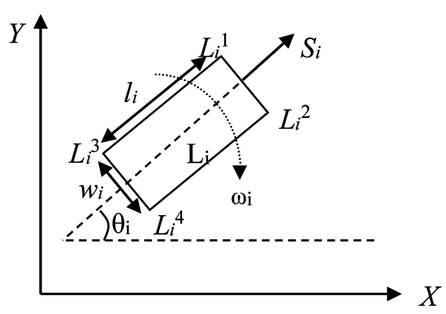The linear speed is acceleration controlled with the maximum acceleration/deceleration of a^max_i. The orientation is controlled by the angular speed. The speed setting, as specified by the algorithm, is assumed to be fast and precise. Fuzzy systems can handle imprecision and take corrective actions to combat any uncertainties. Hence the general navigation of the vehicle will not be affected by the uncertainties in speed setting. However the decision of whether to overtake or not, assumes precise speed settings under a small threshold. The vehicle is assumed to be rectangular of dimensions l_i × w_i with four corners denoted by: front-left L_i¹, front-right L_i², rear-left L_i³ and rear-right L_i⁴. The various notations have been summarized in Figure 1.

Figure 1. Basic notations of the vehicle.

Figure 1. Basic notations of the vehicle.

The basic problem is to plan the immediate movement of the vehicles involved. It is expected that each vehicle maintains some minimal distances from both other vehicles and obstacles from the front and side. The maintenance of a safety distance ensures that a vehicle would have sufficient time to come to a halt or move to another lane in case the vehicle in front suddenly stops. The safety distance of front d_f and side d_s may be given by Equation (1).

d_f = c₁ v_i²
d_s = c₂ v_i²

(1)

Here c₁, c₂ are constants, c₁ > c₂. Assume that the autonomous vehicle sees an obstacle in front which cannot be avoided. In such a case the emergency braking module of the autonomous vehicle will be activated, leaving the operation of the standard planning module. Assuming a maximum deceleration of a^max_i, the distance required for the vehicle to stop while operating at the speed of v_i is v_i²/2 a^max_i. This distance is not realizable due to reaction time, imperfect deceleration, uncertainties in sensing and actuation, etc. Hence the term is discounted by a factor. The discounted term along with the maximum acceleration constitute the term c₁. Even though there is no “side acceleration” of a vehicle and even though obstacles to the side never actually collide with the vehicle, there is a chance that an obstacle to the side may in fact be a road boundary which may exhibit a gradual curve and thus ultimately come ahead of the vehicle. A similar projection is hence applied to obstacles to the side.

We further assume that the same road is used for both inbound and outbound traffic with (in general) half the road for each side. It is assumed that the “left side” driving rule is followed. However the road may not have physical barriers separating the two sides and it is possible to partly occupy the wrong side of the road in order to perform an overtaking procedure.

The fuzzy system largely requires the positions and velocities of the vehicles around, and primarily if the vehicles are in the close vicinity. The perception systems onboard can perceive the position and speed information of the surrounding vehicles clearly, even though the uncertainties may be very high for those vehicles which are far away. The reactive methodology is itself best to deal with the uncertainties, as only the immediate motion of the vehicles is decided based on the current percepts. As the vehicle gets closer to any obstacles, speed and position information gets clearer, and correspondingly better collision-avoidance actions are made.

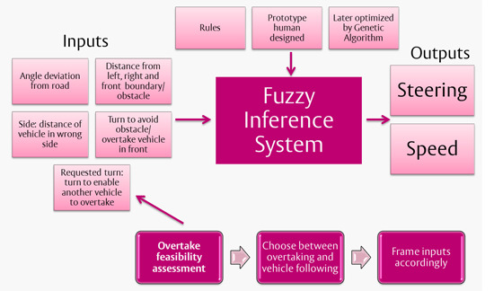
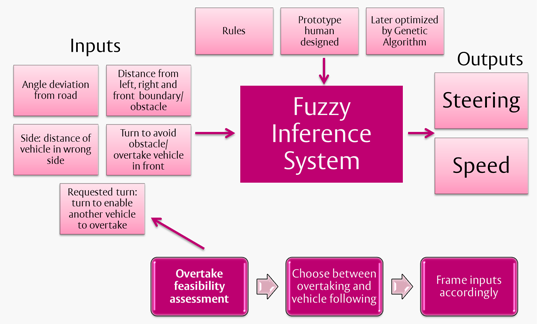
4. Fuzzy Inference System

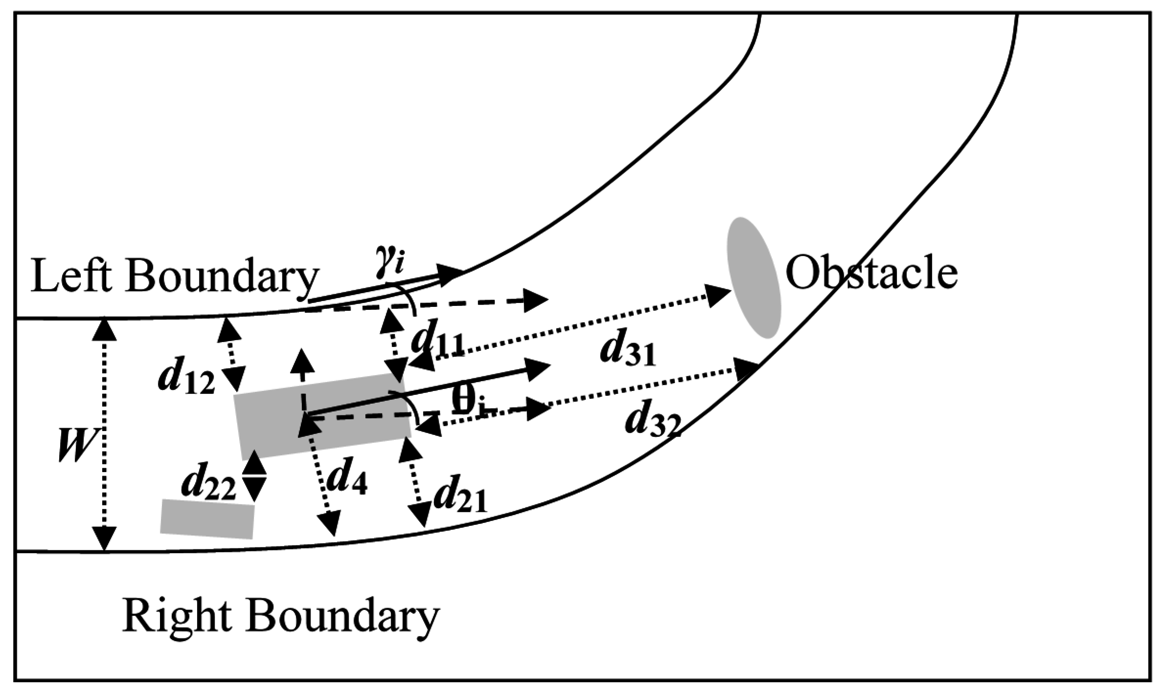
The fuzzy system is given the immediate scenario, for which it tries to plan the immediate movement of the vehicle. The fuzzy system developed is given a total of seven inputs. These include five continuous inputs and two discrete inputs. The intention is to drive along the orientation of the road. The first input is the angle between the road γ_i and the current orientation θ_i (Equation (2)). Normally a vehicle is driven parallel to the road boundary. If the road boundary is curved, the driver steers so as to produce the same curve in the trajectory of the vehicle, always nearly keeping the vehicle placed parallel to the road boundary. The input records any deviation of the vehicle’s heading direction with that of the direction of the road boundary so that the fuzzy rules can try to correct it. The angle γ_i is computed as the slope of the boundary that lies nearer to the vehicle. The various notations are also given in Figure 2.

I_i¹ = γ_i − θ_i

(2)

The next two inputs to the fuzzy system are the distance of the vehicle from the left (and right) boundary or the obstacle/other vehicle on the left (and right). It is always risky to travel very close to the road boundary or having another vehicle very close on the left (or right). Human drivers normally drive so as to maximize the lateral separations. These inputs ask the fuzzy rules to attempt to maximize the distances from both the left and right. In the limiting cases, when the vehicle has the maximum lateral separation, the effect of both the rules cancel each other out. The distances are measured from both of the corners and the smaller distance is used. The safety distance is subtracted. Let d₁₁ be the distance of the obstacle from the front-left corner of the vehicle (L_i¹). Let d₁₂ be the distance from the rear-left corner of the vehicle (L_i³). The input from the left (I_i²) is then given by Equation (3). Correspondingly the input from the right (I_i³) is given by Equation (4). The various notations are shown in Figure 2.

Figure 2. Various inputs to the fuzzy based planner.

Figure 2. Various inputs to the fuzzy based planner.

I_i² = min{d₁₁, d₁₂} − d_s

(3)

I_i³ = min{d₂₁, d₂₂} − d_s

(4)

The next input is the distance from the road boundary or obstacle directly ahead. The input asks the vehicle to steer so as to avoid the obstacle directly ahead, and to slow down so as to avoid any collision if a timely steer is not possible. A moving vehicle need only be considered if it has a negative relative velocity or if there is the potential for a collision to occur. Alternatively the two vehicles should be travelling on opposite sides of the road. Let d₃₁ be the distance of the obstacle from the front-left corner of the vehicle (L_i¹) and let d₃₂ be the distance from the front-right corner of the vehicle (L_i²). The input from the front (I_i⁴) is given by Equation (5).

I_i⁴ = min{d₃₁, d₃₂} − d_f

(5)

The next input is a discrete input called steer to avoid obstacle. Assume that an obstacle (or moving vehicle) lies directly in front. Now the vehicle needs to decide whether to overtake/avoid the obstacle on its left or right side. This input I_i⁵ is given by Equation (6).

$$I_i^5=\{\begin{array}{c}-1\\ 0\\ 1\end{array}\begin{array}{c}\text{avoid obstacle by steering left}\\ \text{no steering required}\\ \text{avoid obstacle by steering right}\end{array}$$

(6)

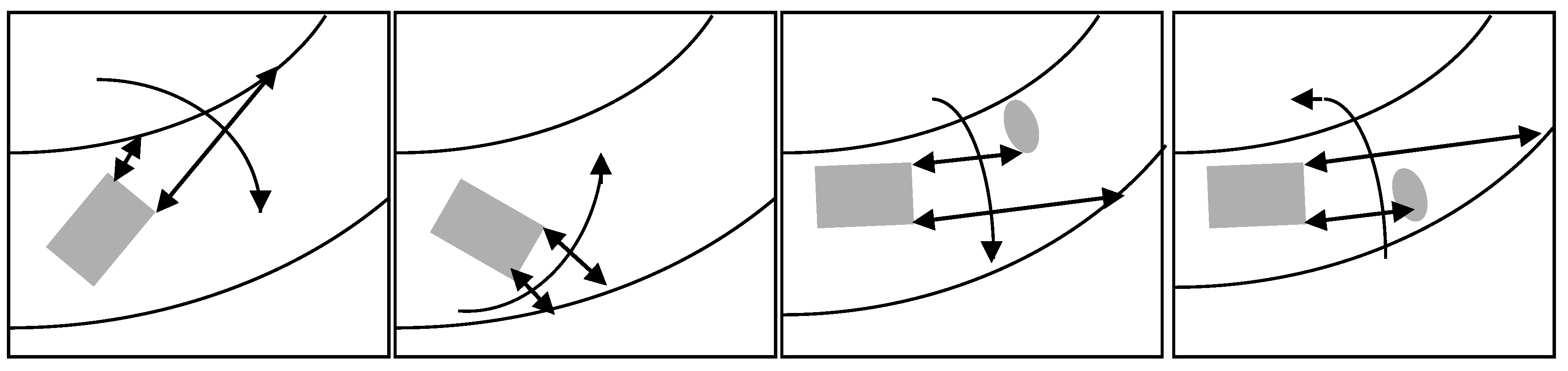
The optimal choice of the input can only be made by deliberative means. One needs to assess the feasibility of all the options by planning and considering future consequences. However here the intention is to make a purely reactive planner and hence heuristics are employed for decision making in real time. In most general cases an obstacle may be aligned so as to indicate the required steering correction. Road curvature also indicates the steer necessary. The two distances measured from the forward obstacle are used to assess the obstacle orientation and hence the turn required. If the left distance is less, the obstacle may be aligned such that a right steer is preferable and vice versa. Numerous cases are shown in Figure 3. Static obstacles are rarely seen in traffic. Most static obstacles are small, for which this heuristic holds. The heuristic may not hold for moving vehicles, for which we use an overtaking mechanism as is discussed in Section 5.

Figure 3. Decision making regarding steering left or right.

Figure 3. Decision making regarding steering left or right.

The next input to the system is side which tries to push the vehicle to the left side of the road. This input takes a value as the distance to which the (rightmost part of the) vehicle is shifted from the middle of the road (demarking the left and right sides). The intention is to quickly push the vehicle to its correct side of travel if by chance it happens to slip onto the wrong side. Let W be the immediate width of the road and d₄ be the distance of the centre of the vehicle from the right boundary. The distance of the rightmost part of the vehicle from the left boundary can be approximated by subtracting half the vehicle’s width (w_i). The value of the fuzzy input side I_i⁶ may hence be given by Equation (7).

$$I_i^6=\{\begin{array}{cc}W/2-\left(d_4-w_i/2\right)& {\text{if d}}_4-w_i/2<W/2\\ 0& otherwise\end{array}$$

(7)

The next input is another discrete input called requested steer. This is an input introduced to enable vehicles to coordinate. It may be beneficial, on many occasions, for a vehicle to the rear to have the vehicle in front steer to the left or right. This mostly happens in overtaking, when the steering of a vehicle in front may make an overtaking option easier or even may make an infeasible overtaking option feasible. A vehicle is thus allowed to request any other vehicle to steer towards either side as an act of cooperation. The possible values of the input are given by Equation (8).

$$I_i^7=\{\begin{array}{c}-1\\ 0\\ 1\end{array}\begin{array}{c}\text{requested to steer left}\\ \text{no steer requested}\\ \text{requested to steer right}\end{array}$$

(8)

The fuzzy system gives as output the linear speed and angular speed necessary for operation. The fuzzy rules can be built along the lines of the thought process and instincts of professional drivers.

5. Overtaking

During driving, whether to overtake a vehicle in front or not is an important decision. A reactive system may not be able to model such a phenomenon. Hence a separate mechanism has been designed. Currently, if a faster vehicle is behind a slower vehicle, the faster vehicle would detect the slower vehicle as an obstacle and avoid it. Unfortunately if there was another slow vehicle in the possible overtaking lane, or an oncoming vehicle, then overtaking at that time would be infeasible. In such a case it is expected for the vehicle to follow the slower vehicle in front.

The feasibility of overtaking can be decided on the basis of the speeds and positions of the vehicles involved. It is further assumed that the vehicles continue to travel straight with their same speeds if overtaking is attempted. Since the decision is to be made in real time, it may not be possible to simulate the system in any way to decide on the feasibility. An assumption is made that the road is not wide enough to accommodate more than three vehicles simultaneously.

Let the vehicle initiating the overtaking be V_i. Let the vehicle being overtaken be V_j. In order for the overtaking to be feasible it is mandatory that V_i should be able to come with a trajectory such that while overtaking it does not collide with V_j. Further it is mandatory that during the motion V_i should not collide with any other vehicle V_x in the scenario. The feasibility is given by Equation (9).

$$Feasible=Feasibl{e}_2(V_i,V_j){\wedge }_{\text{x,x}\ne {\text{V}}_{\text{i}}{\text{,V}}_{\text{j}}{\text{.V}}_{\text{x}}{\text{ ahead of V}}_{\text{i}}}Feasibl{e}_3(V_i,V_j,V_x)$$

(9)

Feasible₂ (V_i, V_j) is a measure of the possibility of overtaking being performed between a faster V_i and a slower V_j ahead. For this it is essential that the road must be wide enough to accommodate both V_i and V_j during the overtaking period with some lateral safety margin φ on both sides. The point of overtaking may approximately be taken as the current location of V_j. Let the length of the two vehicles be l_i and l_j, widths be w_i and w_j and let the width of the road be W. The feasibility is given by Equation (10).

Feasible₂ (V_i, V_j) = w_i + w_j + 2φ ≤ W

(10)

Feasible₃ (V_i, V_j, V_x) measures the feasibility of overtaking by considering the three vehicles V_i, V_j and V_x (≠V_i, V_j). In order for overtaking to be feasible, it is necessary that the road must be wide enough that the three vehicles may all fit in easily. Alternatively the longitudinal separation along the length of the road must be large enough that V_i can overtake V_j while V_x is not yet in the overtaking zone. We need to measure the relative speeds and distances for formulating the feasibility condition due to longitudinal separation. The total time taken for overtaking is given by Equation (11).

$$t=\frac{\left|\right|L_i-L_j|{|}_L+l_i/2+l_j/2}{v_i-v_j}$$

(11)

Here ||.||_L measures the distances between the vehicles in the longitudinal direction, along the length of the road.

In case V_x is travelling in the same direction as V_i and V_j (all inbound or all outbound), the relative speed of V_x with respect to V_j is given by v_x − v_j. In case V_x is travelling in the opposite direction to V_i and V_j (overtaking is being attempted partly using the wrong side) the relative speed is given by v_x + v_j. The distance travelled by the vehicle V_x may hence be given by Equation (12).

$$D=\{\begin{array}{cc}(v_j-v_x)t& \text{same side of travel}\\ (v_j+v_x)t& \text{opposite side of travel}\end{array}$$

(12)

The vehicles are stated to be longitudinally well apart to avoid a collision if the final separation between the vehicles V_j and V_x is large enough to sufficiently accommodate the complete length of the overtaking vehicle V_i. The net feasibility is then given by Equation (13).

Feasible₃(V_i, V_j, V_x) = w_i + w_j + w_x + 6φ ≤ W ∨|| L_j − L_x ||_L − D > l_i + 2Δ

(13)

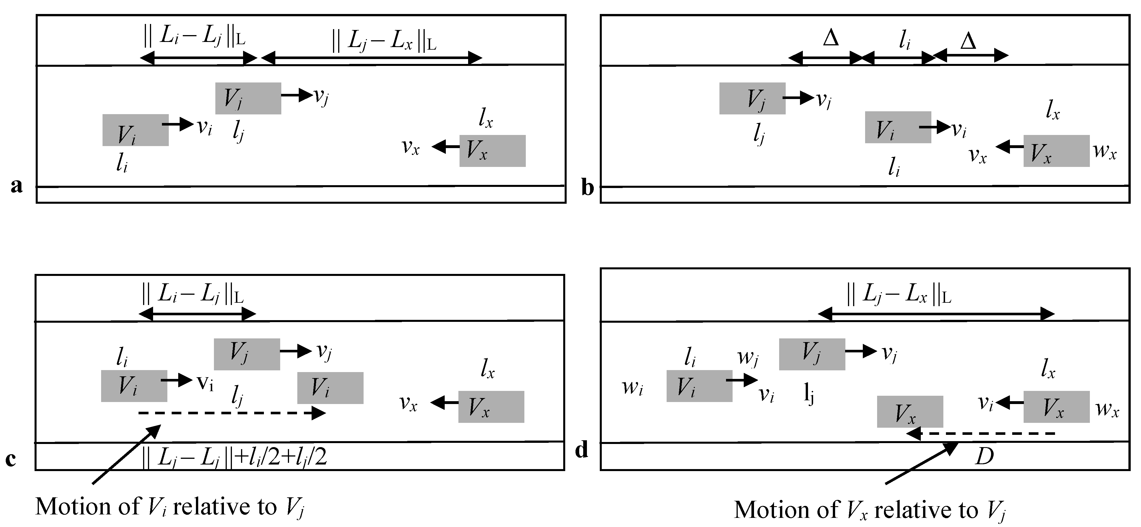
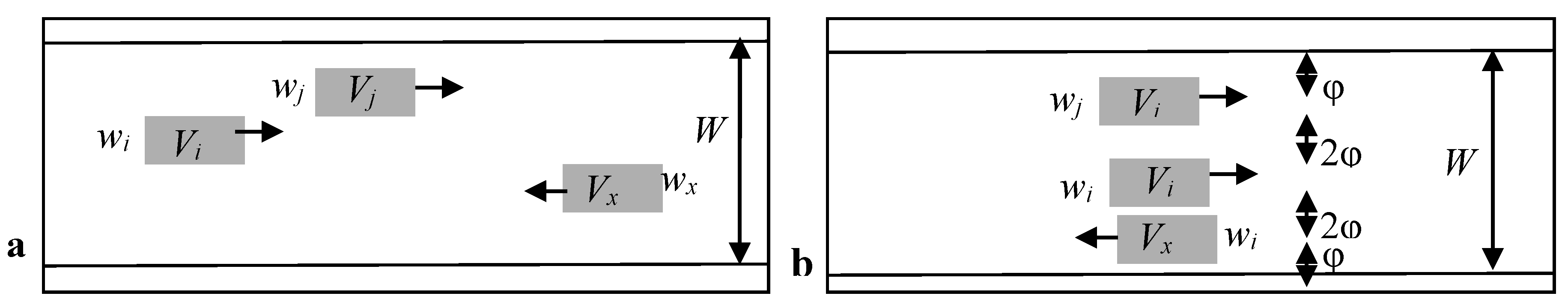
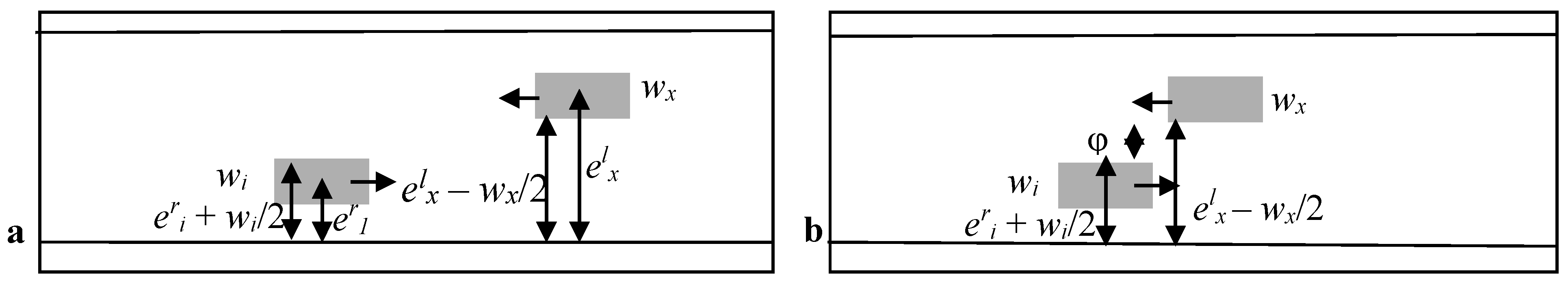
Here φ and Δ are the safety distances in the lateral and longitudinal directions. The various notations are illustrated in Figure 4 for the case where the width of the road is enough to enable overtaking for the three vehicles and Figure 5 for the case where the longitudinal separation of the three vehicles is enough to enable the overtaking to take place.

Figure 4. Notations for deciding feasibility of overtaking when three vehicles can be accommodated within the road width: (a) Initial Positions; (b) Final Positions.

Figure 4. Notations for deciding feasibility of overtaking when three vehicles can be accommodated within the road width: (a) Initial Positions; (b) Final Positions.

Figure 5. Notations for deciding feasibility of overtaking when three vehicles have enough longitudinal separation: (a) Initial Positions; (b) Final Positions; (c) Motion on V_i relative to V_j; (d) Motion on V_x relative to V_j.

Figure 5. Notations for deciding feasibility of overtaking when three vehicles have enough longitudinal separation: (a) Initial Positions; (b) Final Positions; (c) Motion on V_i relative to V_j; (d) Motion on V_x relative to V_j.

If overtaking turns out to be feasible, the next task is to decide on the motion of each of the participating vehicles. We first decide whether V_i should preferably overtake V_j on its left side or right side. This is done by analyzing the distance V_i would be required to move for both the possible cases and the lesser one is then used. The preferred direction of motion of V_j is set to the converse of that of V_i. For V_i the computed direction is given as the input to the steer variable of the fuzzy planner (I_i⁵). For V_j, the computed direction is given as input to the requested steer variable (I_j⁷). The task needs to be performed for all other vehicles with which the feasibility was checked. We firstly check if there is any requirement of the other vehicles to steer in a specific manner. In case there is no need to steer for V_x, the entire overtaking procedure is said to be non-cooperative. However in case V_x needs to move to give some extra space to the overtaking vehicle, overtaking is referred to as being cooperative.

Overtaking may be cooperative only when the longitudinal distance computed was not large enough. In case the road width is large enough, the vehicles would treat each other as obstacles and steer automatically. When the steer is cooperative V_x steers in the direction opposite to the direction of V_i and V_j. The steer is un-cooperative if there is enough space for both the vehicles to drive through without the movement of V_x. Consider the case that V_x is travelling in the opposite direction to V_i and V_j. The need for cooperation is given by Equations (14) and (15).

Coop₁(V_i, V_j, V_x) = (e^l_x − w_x/2 < e^r_i + w_i/2 + φ∨e^l_x − w_x/2 < e^r_j + w_j/2 + φ)∧ || L_j − L_x ||_L − D < l_i + 2Δ

(14)

Coop₂(V_i, V_j, V_x) = (e^r_x − w_x/2 < e^l_i + w_i/2 + φ∨e^r_x − w_x/2 < e^l_j + w_j/2 + φ)∧ || L_j − L_x ||_L − D < l_i + 2Δ

(15)

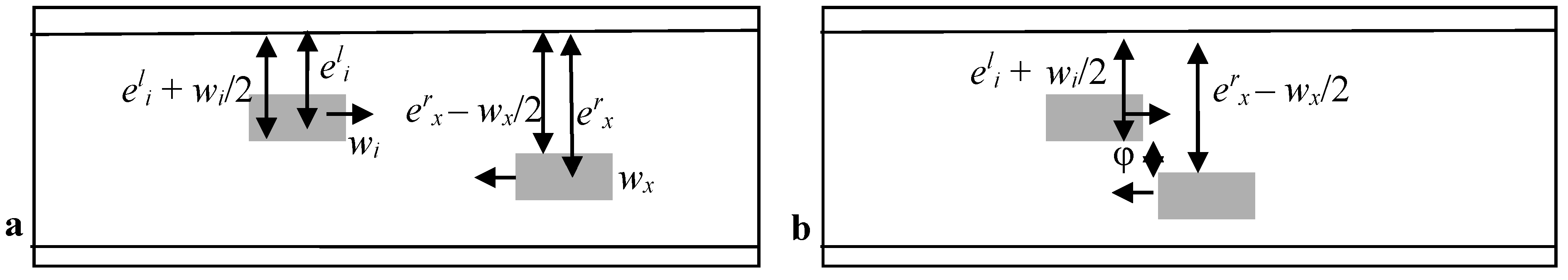
Here e^l_x denotes the distance of the centre of V_x from the left boundary (relative to itself) and e^r_x denotes the distance of the centre of V_x from the right boundary (relative to itself). The closest distances to the vehicle from the boundaries are approximated by adding/subtracting half the vehicle’s width. Overtaking is cooperative if either Equation (14) or (15) computes to be true. In case Equation (14) is true the steer is cooperative and R_x is expected to steer towards its right. In case Equation (15) is true, R_x is expected to steer left. The various notations are given in Figure 6 for Equation (14) and Figure 7 for Equation (15). The notations of V_j (not shown in the figures) are similar to those of V_i.

Figure 6. Notations for deciding the turn of V_x with V_i overtaking V_j. Case involving right turn: (a) Initial Positions; (b) Overtake Positions.

Figure 6. Notations for deciding the turn of V_x with V_i overtaking V_j. Case involving right turn: (a) Initial Positions; (b) Overtake Positions.

Figure 7. Notations for deciding the turn of V_x with V_i overtaking V_j. Case involving left turn: (a) Initial Positions; (b) Overtake Positions.

Figure 7. Notations for deciding the turn of V_x with V_i overtaking V_j. Case involving left turn: (a) Initial Positions; (b) Overtake Positions.

On many occasions a faster vehicle may be forced to slow down and follow a slower vehicle if overtaking is not immediately possible. The above equations allow overtaking to take place only if the vehicle initiating overtaking has a higher speed than the vehicle being overtaken. In such a scenario overtaking still may not necessarily take place. For this we place an exception that a vehicle capable of overtaking may overtake if no other vehicle lies ahead in the vicinity. A vehicle is capable of overtaking if its maximum speed is greater than the speed of the slower vehicle ahead. The condition Feasable₂ (V_i, V_j) must however be true. Although clearly travelling in the same direction, laterally, the two vehicles move in opposite directions to enable overtaking. V_i in its course of overtaking would increase its speed. While overtaking is being initiated, we keep the left side preferred rule deactivated (by always giving an input of 0 to the corresponding fuzzy input I_i⁶) as well as considering the front obstacle distance to be infinitely large. This however is only for the initiation of overtaking. Once the vehicle has laterally crossed the vehicle being overtaken, in other words when the two vehicles are in different lanes, both the features are enabled again.

The overtaking mechanism employed here is inspired by general driving of today. If a vehicle sees the possibility of overtaking which requires the cooperation of other vehicles it sends a signal in the form of a horn, or the overtaking gesture is visually perceived by the other vehicles around. The other vehicles hence know about the overtaking attempt and can align themselves in a manner so as to allow overtaking to take place.

6. Going over/through a Crossing

The last feature of the algorithm is the mechanism of passing over a road crossing. Virtual barricades are drawn over the road on which the vehicle is not supposed to move. This effectively converts the crossing region into a continuous (maybe curved) road segment bounded by real and virtual boundaries at both ends. Crossings with roundabouts are much simpler where such boundaries are prominent. This is shown by Figure 8. Traffic lights, if present, carry out the task of coordination. For crossings without lights, we maintain a first-come-first-serve system of motion.

Figure 8. Use of virtual barricades for crossing scenario.

Figure 8. Use of virtual barricades for crossing scenario.

The other major restriction while at or near a crossing is that the overtaking module is completely disabled and vehicles need to follow each other, i.e., no overtaking is allowed over a road crossing. Further, no vehicle may ask another vehicle to itself steer left or right. Allowing overtaking at or near a crossing scenario might result in traveling over the stop lines if overtaking is not completed in time.

7. Evolution of the Fuzzy Inference System

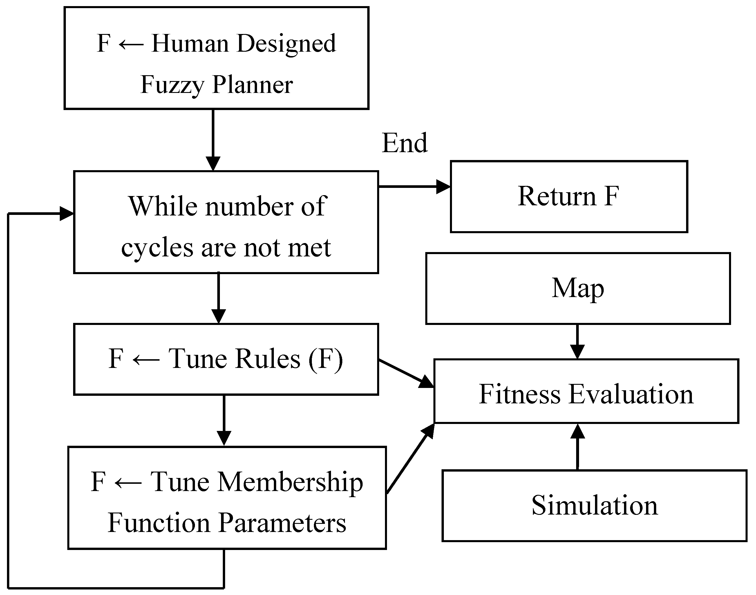
Complete evolution of the fuzzy system is not possible due to the complexity of the problem. Evolution of the fuzzy inference system is a complex and time consuming task. It cannot be done in near-real time based on the navigation profile of the vehicle. The intention is to evolve a fuzzy inference system completely offline based on the simulated model of the vehicle. The evolved fuzzy inference system is then used for the navigation of the physical vehicle, during which no learning takes place. This allows the vehicle to navigate at high speeds by reacting to the different obstacles and changes in the environment. Hence a prototype fuzzy system was initially manually designed by heuristics and trial and error. The system was simulated on multiple paths with anomalies in the motion being noted and iteratively rectified by tuning or adding membership functions and rules. Evolution is then restricted around the prototype fuzzy system so produced. Evolution is used for the tuning of the rules and membership functions. Evolution is carried forward in cycles. First the evolutionary process tried to tune the rules for some generations. This produces a fuzzy system that has better rules. The next task is to optimize the membership function as per the requirements of the new set of rules generated. The whole process was repeated for a few cycles. The search space of each of the two evolutionary processes is limited. The complete evolutionary process is summarized in Figure 9.

Figure 9. Evolution of the fuzzy planner.

Figure 9. Evolution of the fuzzy planner.

Tuning of the rules is the first half of the problem. Evolution is allowed only to increase or decrease the participating membership function of any antecedent or consequent in the best fuzzy system (so far) by a unit value. Hence in the best fuzzy system for any rule if an antecedent/consequent has a participating membership function “high”, the evolutionary process can change it to “low” or “very high”, provided both are existent. The genotype consisted of a string of integers which may be either −1, 0 or +1. In all there are R(I + O) integers. Here R is the number of rules, I is the number of inputs and O is the number of outputs. A − 1 means the corresponding input’s/output’s membership function is to be decreased by one and similarly for +1 and 0. The negative membership function numbers denote use of a NOT operator.

Optimization of the membership functions is the second task. Hence again in order to keep the fitness landscape limited, we restrict the search domain to a small percentage around the present value. The individual representation in this case is simple. All the membership functions are noted and their parameters appended one after the other.

Conventional genetic operators are used in both the evolution of the rules and the membership functions. The choice for the evolution is rank based fitness scaling, stochastic universal selection, scattered crossover, Gaussian mutation, and an elite operator.

Evolution is performed on a set of benchmark maps. These maps cover a wide variety of scenarios that the vehicle may face in real life. The fitness is the mean performance of the vehicle in all these maps. We aspire to make all vehicles travel along their respective paths in as little time as possible. Penalties are added for not maintaining safety distances from the front and side, for colliding and for driving on the wrong side of the road. The entire fitness function for any individual is given by Equation (16).

$$fit=\frac{{\displaystyle \sum _{i=1}^{np}\raisebox{1ex}{${\displaystyle \sum _{j=1}^{n{v}_i}(t_{ij}+p_1.collid{e}_{ij}+p_2.(safe{1}_{ij}+safe{2}_{ij})+p_3.sid{e}_{ij})}$}\!\left/ \!\raisebox{-1ex}{$n{v}_i$}\right.}}{np}$$

(16)

Here np is the number of maps used for learning and nv_i is the number of vehicles used in the i^th map. For the i^th map and the j^th vehicle in the map t_ij is the time taken to travel; collide_ij is the distance left for the vehicle to travel if the vehicle collides before completing the journey, 0 otherwise; safe1_ij and safe2_ij are the margins by which the front and side safety margins are disobeyed; and side_ij is the average distance that the vehicle stays in the wrong side. p₁, p₂ and p₃ are the penalty constants. To compute these factors, we extend the Equations (3) – (5) and (7) to compute the fuzzy inputs. safe1_ij and safe1_ij are given by Equation (17) and side_ij is given by Equation (18).

safe1_ij(t) = max(F_s − min{d₁₁, d₁₂}, F_s − min{d₂₁, d₂₂},0)
safe1_ij = max_t(safe1_ij(t))
safe2_ij(t) = max(F_d − min{d₃₁, d₃₂}, 0)
safe2_ij = max_t(safe2_ij(t))

(17)

$$sid{e}_{ij}=\frac{{\displaystyle \underset{t=0}{\overset{t_{ij}}{\int }}{I}_6^i(t).dt}}{t_{ij}}.$$

(18)

8. Results

The simulations were performed in MATLAB. The simulation setup was entirely created by the authors for the work. The prototype fuzzy system was manually designed. For the optimization of the prototype fuzzy system, a total of five cycles were applied with a population size of 20 individuals and 20 generations as the stopping criterion. The crossover rate was 0.8 and an elite count of 2 was used. This produced the final fuzzy planner used for the simulations. The next task was to generate a number of scenarios and to simulate a group of vehicles. The results are better illustrated in the supplementary video. The units of both distance and time are arbitrary and specific to the simulation tool. These relate to the real world units by constants. Consider that one simulation unit distance (pixel) is 8 cms. Further consider that one simulation unit time is 0.05 s. The vehicles by this relation are of size 3.2 m× 3.2 m. (including annexures like mirrors, excluding safety distances). The experiments involved a maximum speed limit of 16 m/s or 57.6 Km/h. The average road length varied from 48 meters to 62 meters. The average road width varied from 13 meters to 16 meters. The intention behind the experiments was unorganized traffic, wherein the traffic does not adhere to lane discipline. Hence the roads were not divided by lanes. Some of the roads could accommodate two vehicles comfortably (along with comfortable safety distances), while some others could accommodate up to three vehicles (with modest safety distances). The vehicles were expected to drive in such non-lane oriented traffic, judging whether it would be possible to squeeze in-between vehicles or to wisely follow a vehicle and wait for an overtaking opportunity.

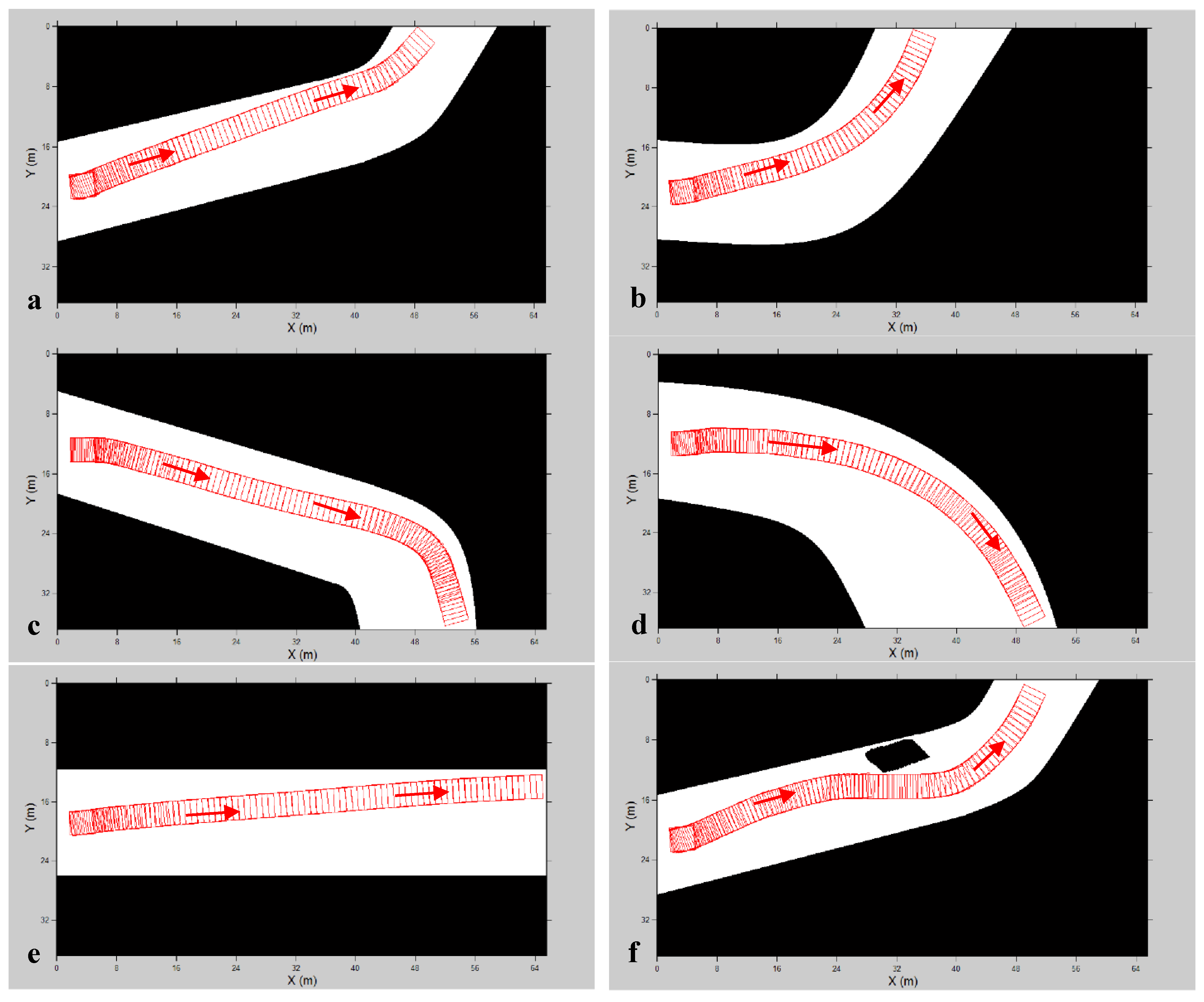
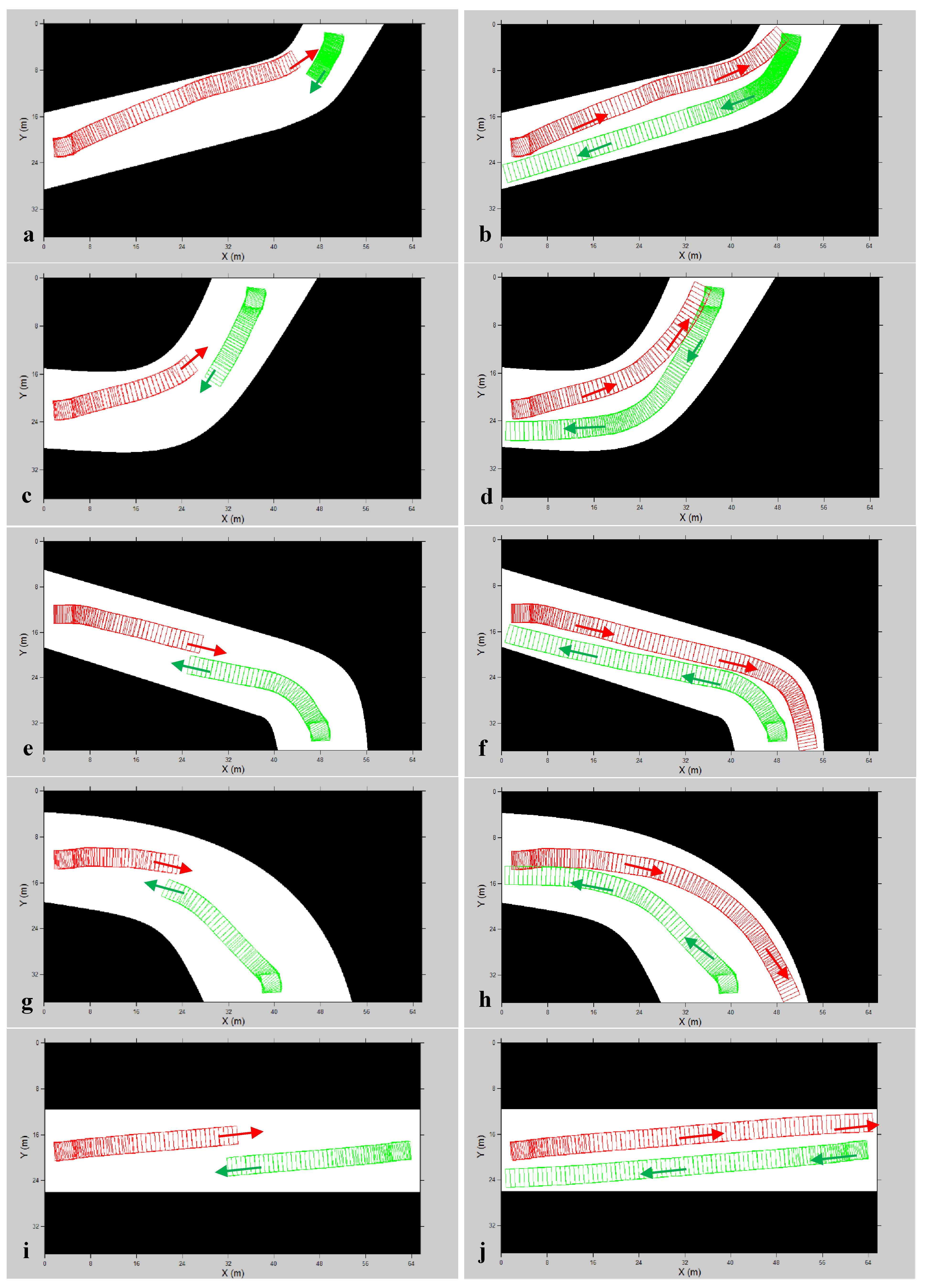
First we simulated the system with a single vehicle. The result for different scenarios is presented in Figure 10. The scenarios make the vehicles turn both left-ward and rightward in order to stay on the left of the road and avoid any obstacles. In all cases the vehicle could easily navigate its way without collision. The next scenarios were with two vehicles travelling on opposite sides of the road, heading directly towards each other. The challenge for either of the moving vehicles was hence increased as they had to avoid each other. The results are shown in Figure 11. Odd numbered figures show the scenario when the vehicles avoid each other, while the even numbered figures show the scenario at the end of the simulation.

Figure 10. Simulation results with one vehicle. (a) First Left Turn Scenario; (b) Second Left Turn Scenario; (c) First Right Turn Scenario; (d) Second Right Turn Scenario; (e) Straight Road Scenario; (f) Obstacle Avoidance Scenario.

Figure 10. Simulation results with one vehicle. (a) First Left Turn Scenario; (b) Second Left Turn Scenario; (c) First Right Turn Scenario; (d) Second Right Turn Scenario; (e) Straight Road Scenario; (f) Obstacle Avoidance Scenario.

Figure 11. Simulation results with two vehicles. (a) First Left Turn Scenario (midway); (b) First Left Turn Scenario (end of simulation); (c) Second Left Turn Scenario (midway); (d) Second Left Turn Scenario (end of simulation); (e) First Right Turn Scenario (midway); (f) First Right Turn Scenario (end of simulation); (g) Second Right Turn Scenario (midway); (h) Second Right Turn Scenario (end of simulation); (i) Straight Road Scenario (miday); (j) Straight Road Scenario (end of simulation).

Figure 11. Simulation results with two vehicles. (a) First Left Turn Scenario (midway); (b) First Left Turn Scenario (end of simulation); (c) Second Left Turn Scenario (midway); (d) Second Left Turn Scenario (end of simulation); (e) First Right Turn Scenario (midway); (f) First Right Turn Scenario (end of simulation); (g) Second Right Turn Scenario (midway); (h) Second Right Turn Scenario (end of simulation); (i) Straight Road Scenario (miday); (j) Straight Road Scenario (end of simulation).

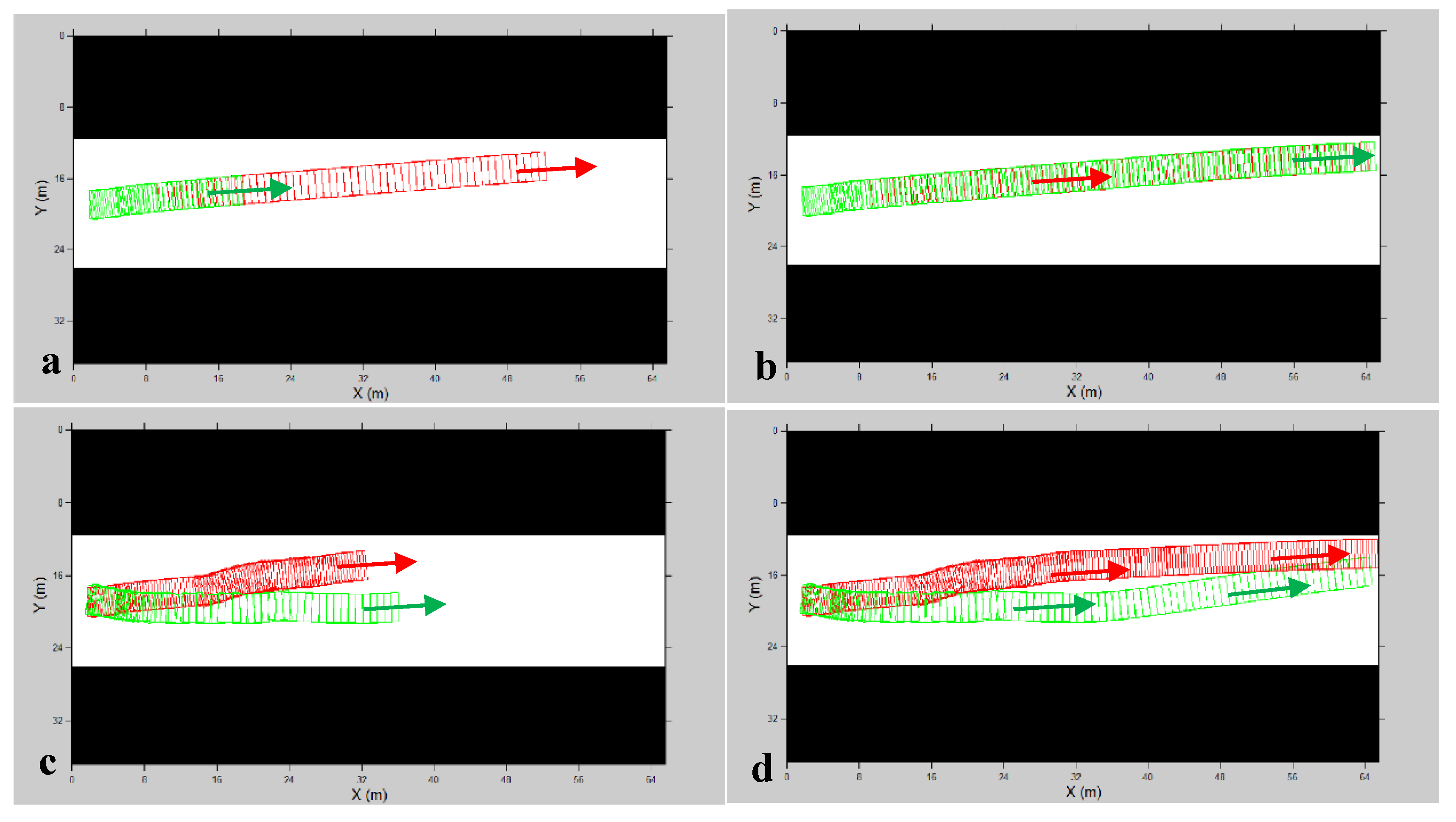
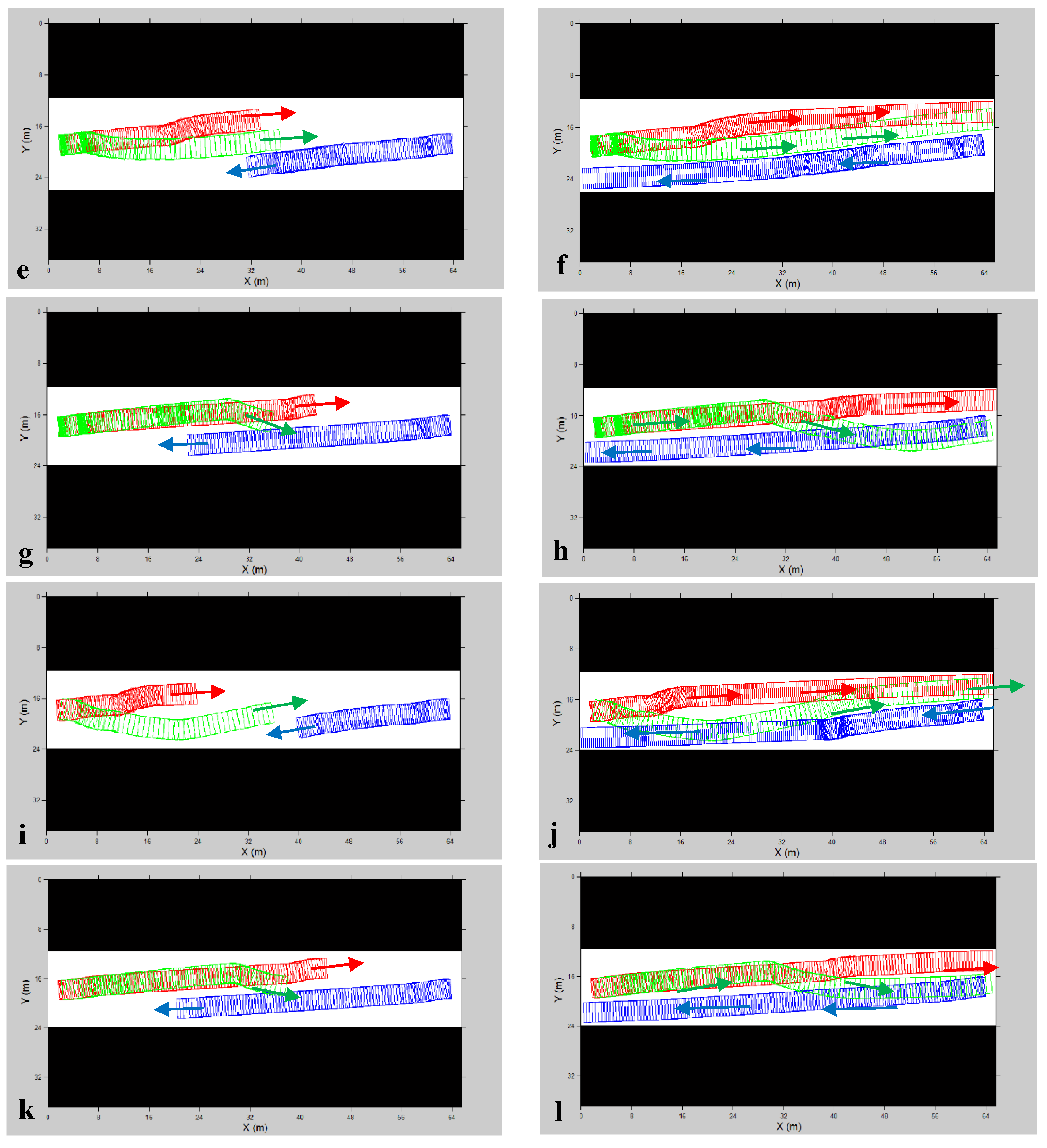
The next set of simulations was used to test the overtaking mechanism of the vehicles. The overtaking of two vehicles and three vehicles were checked independently. In the first scenario (Figure 12a,b) we generated a faster vehicle and made it move on a straight road. After some time a slower vehicle was then produced and was made to move on the same road, behind the faster vehicle. In this case there was no possibility of overtaking taking place. The situation however reversed when we switched the speeds of the two vehicles (Figure 12c,d). In this case it may be easily seen that the faster vehicle, soon saw the possibility of overtaking and initiated the same. The two vehicles steered in opposite (widthwise) directions to each other till there was sufficient distance for the faster vehicle to overtake the slower vehicle.

The next experiments involved three vehicles. Here the experimental setup was done to check the working of the overtaking feasibility equations. First two vehicles entered the scenario at the start and travelled in opposite directions. The third vehicle was made to enter after some time. In the first scenario we considered a map such that the road width was enough to accommodate the three vehicles with sufficient margins. In such a case overtaking was feasible. Overtaking of the vehicle was successfully carried out by the overtaking vehicle, which later returned to its normal lane (Figure 12e,f). We repeated the same experiment with the width of the road decreased. In this case the vehicle decided not to overtake straight away, but instead it initially followed the slower vehicle in front. As soon as the oncoming vehicle passed by, it initiated an overtaking procedure, which was safely executed (Figure 12g,h)).

Figure 12. Simulation results in overtaking scenarios. (a) Vehicle following scenario (midway); (b) Vehicle following scenario (end of simulation); (c) Two vehicle overtaking scenario (midway); (d) Two vehicle overtaking scenario (end of simulation); (e) Scenario with enough road width to host 3 vehicles (midway); (f) Scenario with enough road width to host 3 vehicles (end of simulation); (g) First infeasible overtaking scenario (midway); (h) First infeasible overtaking scenario (end of simulation); (i) Feasible overtaking scenario (midway); (j) Feasible overtaking scenario (end of simulation); (k) Second infeasible overtaking scenario (midway); (l) Second infeasible overtaking scenario 2 (end of simulation).

Figure 12. Simulation results in overtaking scenarios. (a) Vehicle following scenario (midway); (b) Vehicle following scenario (end of simulation); (c) Two vehicle overtaking scenario (midway); (d) Two vehicle overtaking scenario (end of simulation); (e) Scenario with enough road width to host 3 vehicles (midway); (f) Scenario with enough road width to host 3 vehicles (end of simulation); (g) First infeasible overtaking scenario (midway); (h) First infeasible overtaking scenario (end of simulation); (i) Feasible overtaking scenario (midway); (j) Feasible overtaking scenario (end of simulation); (k) Second infeasible overtaking scenario (midway); (l) Second infeasible overtaking scenario 2 (end of simulation).

The next attempt was to test the overtaking decision made when the longitudinal separation between the vehicles was large enough. A number of speed combinations of the vehicles were tried. The cases revolving around the most critical overtaking with the smallest margins are presented. We first examined the case where overtaking was regarded as feasible (Figure 12i,j). The same experiment was repeated with the speeds of the two vehicles initially in the scenario slightly increased. In this case overtaking was infeasible and the faster vehicle decided to follow the slower vehicle. Once the oncoming vehicle passed, overtaking was carried out (Figure 12k,l).

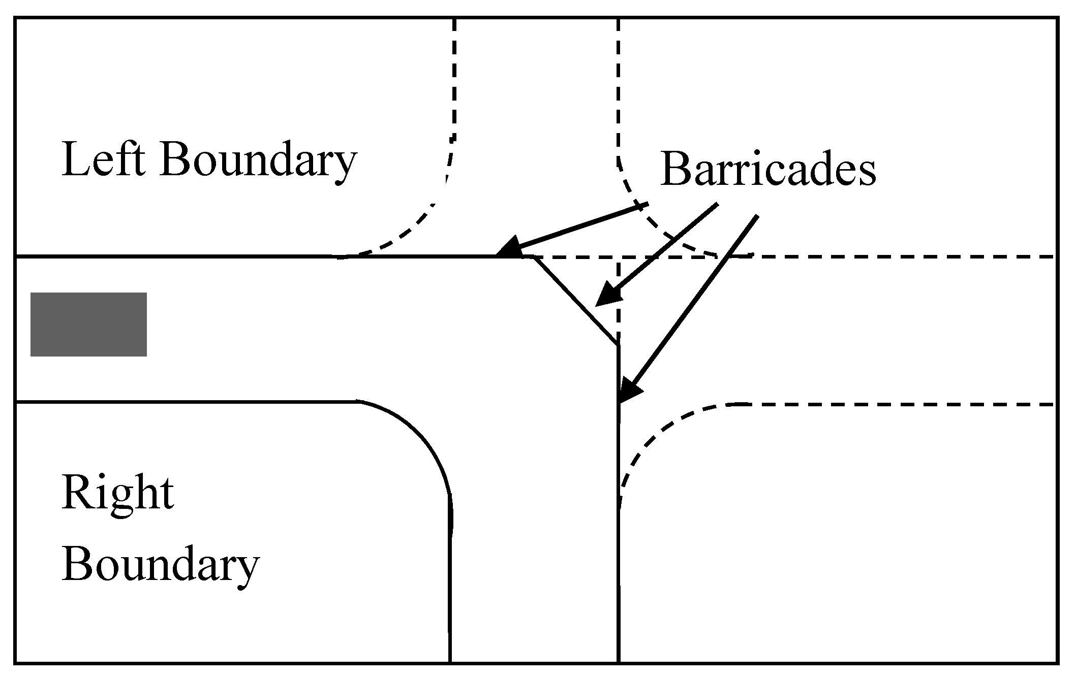
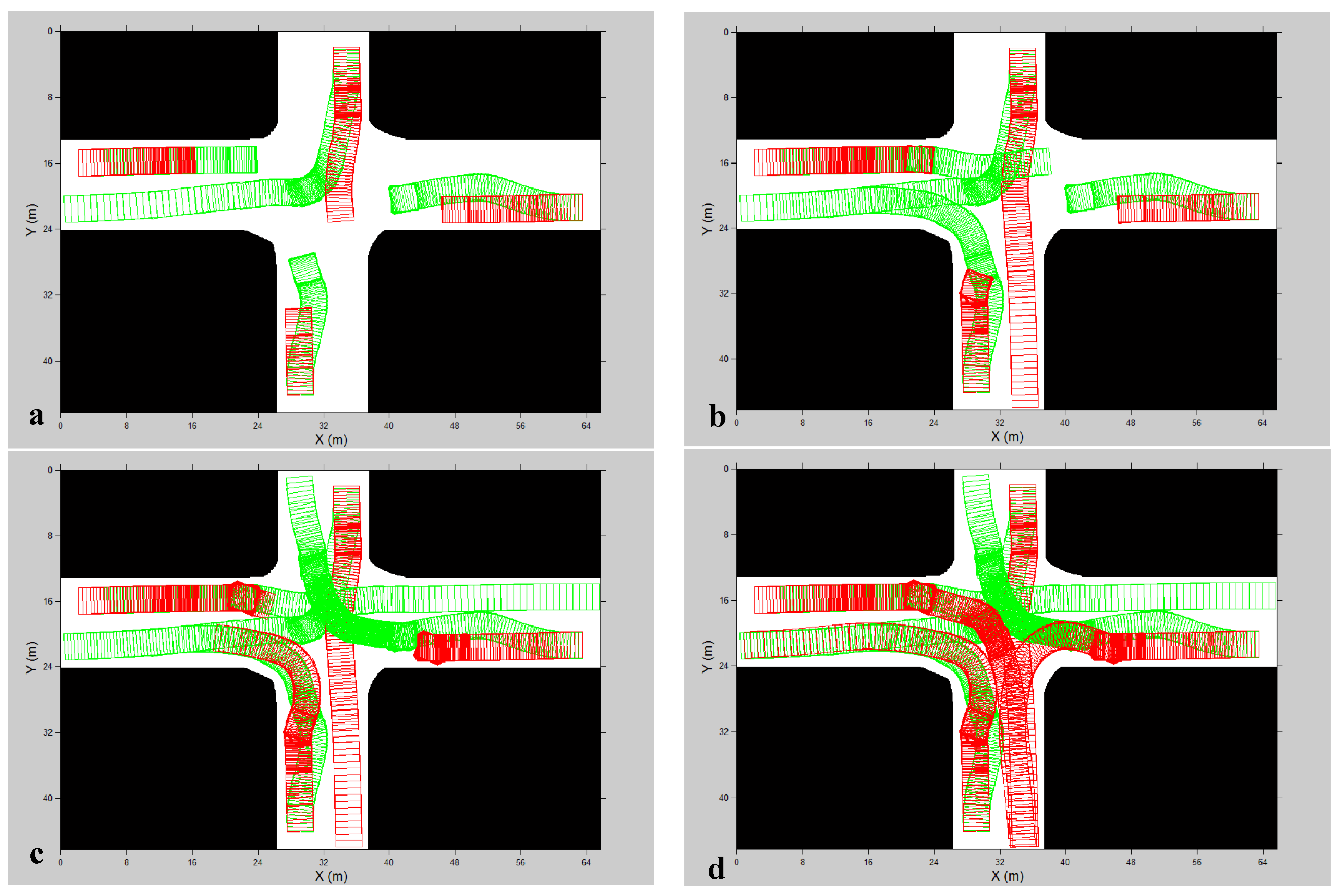
The last simulation was applied to a crossing scenario. A total of eight vehicles were generated, two on each road. All these vehicles were initially travelling at high speed, which they had to reduce slowly after they entered the map. Motion of the vehicles was on a first come first serve basis. The simulation showcased that all vehicles were able to pass each other in a reasonably small crossing time. The resultant path traced by the various vehicles is given in Figure 13.

Figure 13. Simulation results in crossing scenario. (a) t = 6 s; (b) t = 10 s; (c) t = 21 s; (d) t = 29 s.

Figure 13. Simulation results in crossing scenario. (a) t = 6 s; (b) t = 10 s; (c) t = 21 s; (d) t = 29 s.

9. Analysis

The next step involved with the algorithm was to analyze the working of the various mechanisms in the various scenarios. We first considered speed control. The first class of maps involved simple maps with a single vehicle in the path. All units used were arbitrary and specific to the simulation tool. The speed of the vehicle for various scenarios is shown in Figure 14a. Based on the figure it may be easily seen that the greatest acceleration was recorded by the scenarios where the vehicle was supposed to turn left. The simultaneous actions of accelerating and correcting the side of travel put a threshold on the acceleration. The scenario involving an obstacle showed a decrease and increase in speed in the central part of the journey. This enabled the vehicle to overcome the obstacle at a lower speed, upon its sudden emergence.

We further extended the study to cases involving two vehicles. The corresponding graph is shown in Figure 14b. The graph clearly shows that the presence of the other vehicle produced a change in the curves of all the scenarios, except for the one on a straight road; where the two vehicles moved to the correct side fairly early to completely avoid each other. The last case is of overtaking was between three vehicles. We looked at the manner in which the speed changes while a vehicle was overtaking. Here as well we had two scenarios. The first scenario was when the vehicle was allowed to overtake and the second where the vehicle was not allowed to overtake. The speed of the overtaking vehicle in both these scenarios is presented in Figure 14c. The figure shows that the vehicle more or less assumed the maximum speed, which means that overtaking happened at high speed. However in case overtaking was not allowed, the vehicle was supposed to reduce its speed and follow the vehicle ahead for some time, till the oncoming vehicle passed by and overtaking could be achieved. In this case the decrease and re-increase in speed can be seen when overtaking was computed as infeasible. Later the vehicle increased its speed during overtaking.

Figure 14. Relation between speed and time for: (a) scenarios with one vehicle; (b) scenarios with two vehicles; (c) overtaking scenarios.

Figure 14. Relation between speed and time for: (a) scenarios with one vehicle; (b) scenarios with two vehicles; (c) overtaking scenarios.

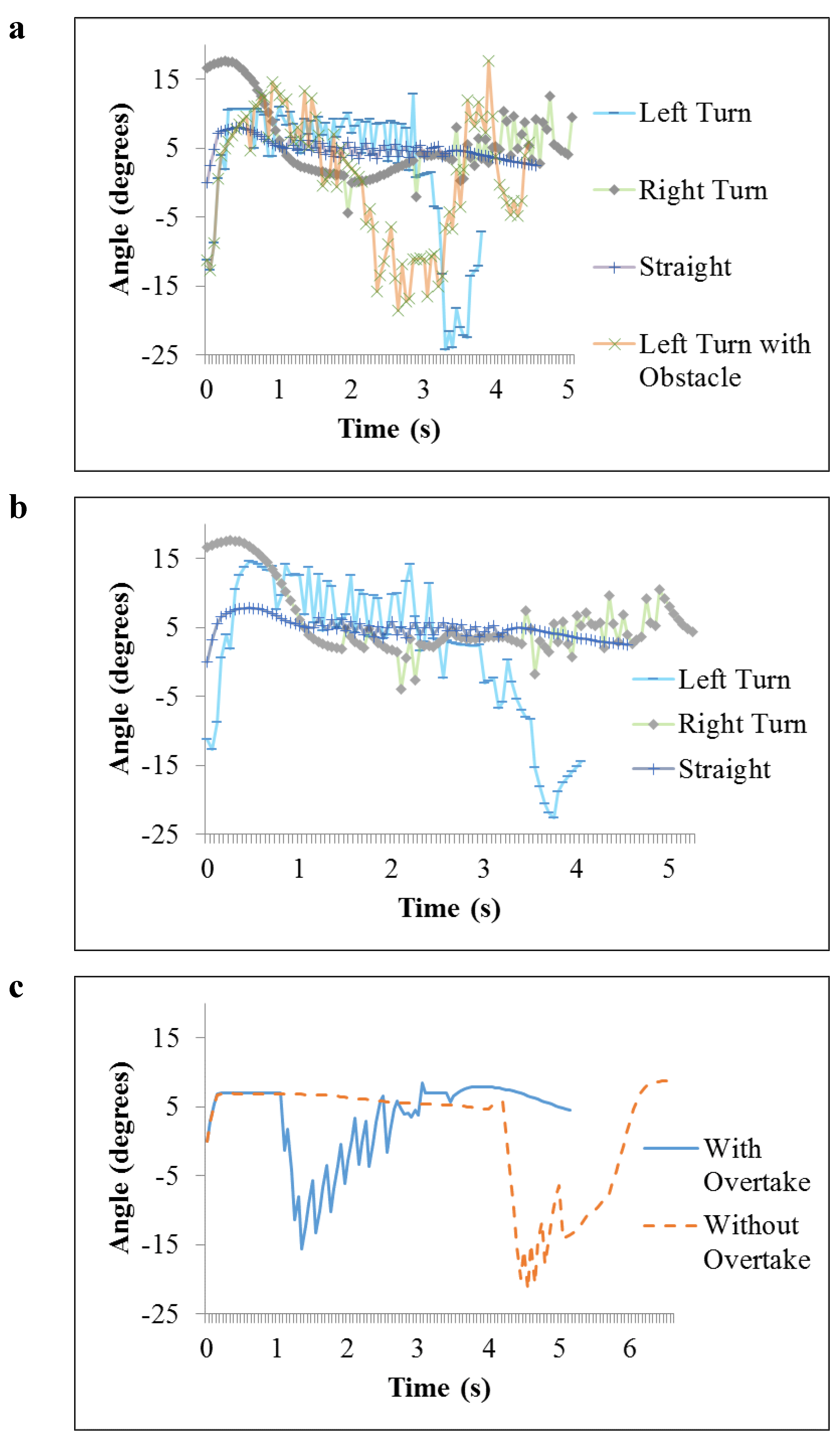
The other part of the analysis was to measure the angle between the orientation of the vehicle and the orientation of the road. For normal driving this angle should be 0. The angle for various scenarios with a single vehicle is shown in Figure 15a. To avoid the graph being too congested only single cases of left and right turn have been plotted. The figure shows that for most cases the angle revolves around 0. There are some oscillations visible to the magnitude of about 5 degrees. The same kinds of observations were visible when we repeated the experiments for the two vehicle scenarios. The plot of angle for different times is given in Figure 15b. The similar nature of the plots indicates that the vehicles could perform some minor steering mechanisms so as to avoid the other vehicle.

Figure 15. Angle difference between orientation of road and vehicle vs. time for: (a) scenarios with one vehicle; (b) scenarios with two vehicles; (c) overtaking scenarios.

Figure 15. Angle difference between orientation of road and vehicle vs. time for: (a) scenarios with one vehicle; (b) scenarios with two vehicles; (c) overtaking scenarios.

The trend however was not the same with overtaking. We studied the scenario of overtaking with three vehicles, when the overtaking vehicle attempted to overtake the vehicle in front of it. The plots for angle with time for the overtaking vehicle are given in Figure 15c. It may be seen that the angle decreased by a large amount and then increased denoting the overtaking. The decrease of the angle below zero was when the vehicle initiated the overtaking and went on the other side of the vehicle being overtaken. Afterwards the angle converged on zero, denoting the attempt to orient the vehicle with the road, while the vehicle being overtaken was still to the side. After overtaking the vehicle attempted to return to its original side, for which the angle became positive, which was controlled and brought towards zero.

Conclusions

The basic motivation of the paper was to plan autonomous vehicles for real time traffic scenarios. Motivated by the basic instincts of professional drivers who drive in such scenarios, we chose to use fuzzy logic for the design of the system. The fuzzy system took as input the status of the surroundings of the vehicle. The fuzzy planner controlled both the steering mechanism as well as the speed. The fuzzy rules carried the task of understanding of the environment and producing the necessary control actions. The fuzzy system was developed and used for planning for a number of roads that ranged from straight roads to roads with steep or smooth turns on either side. Whether to overtake a vehicle or to follow it is a critical question which needs to be answered by assessment of the scenario, and once the decision is made, it is adhered to for some time during driving. In this paper we hence proposed a simple decision making system assuming relatively narrow roads. The decision making system was tested for a number of scenarios.

In the literature the twin problems of assessing an opportunity of overtaking and performing the overtaking maneuver have been done for organized traffic that operates in lanes. So the overtaking procedure is defined as the process to change lanes to the overtaking lane, driving in the overtaking lane, and returning back to the original lane. Also this overtaking procedure is only performed when both the normal driving lane and the overtaking lane have inbound (or outbound) traffic. The paper does not assume clearly defined lanes and also considers that the overtaking lane may have inbound traffic while the normal driving lane has outbound traffic (or vice versa), which means that the overtaking vehicle is forced to slip onto the wrong side to carry the overtaking procedure which is more risky.

The proposed system worked well on the experimental scenarios. However a number of limitations exist which must be addressed in the future. Being a reactive technique the approach is neither guaranteed to be optimal nor complete. For wide roads it may be better not to overtake on some occasions. Similarly, whether driving efficiency is affected or not depends on which side of the road a static obstacle occurs. Currently these decisions are made entirely on a heuristic basis. Better heuristics or the integration of some deliberative means may be useful. Uncertain movements of other vehicles can also make a perfectly feasible overtaking procedure subsequently infeasible, and this needs to be allowed for. The approach needs to be extended to the cases of diversions, mergers, completely blocked roads, etc. This would ensure that the algorithm works as per the discussed lines or, conversely, this may produce new issues to be addressed in the future.