Motion Planning of Autonomous Vehicles on a Dual Carriageway without Speed Lanes

Abstract

The problem of motion planning of an autonomous vehicle amidst other vehicles on a straight road is considered. Traffic in a number of countries is unorganized, where the vehicles do not move within predefined speed lanes. In this paper, we formulate a mechanism wherein an autonomous vehicle may travel on the “wrong” side in order to overtake a vehicle. Challenges include assessing a possible overtaking opportunity, cooperating with other vehicles, partial driving on the “wrong” side of the road and safely going to and returning from the “wrong” side. The experimental results presented show vehicles cooperating to accomplish overtaking manoeuvres.

1. Introduction

Autonomous vehicles [1,2] are capable of driving themselves in traffic scenarios and are seen as a replacement for human-driven vehicles in the future. They make transportation systems efficient and safe [3,4] and are therefore sources of research and development. The problem of planning deals with decision making regarding the motion of a vehicle. Broadly, planning is responsible for the trajectory generation and speed computation of the vehicle at any instance of time. The planning framework enables vehicles to judiciously avoid all obstacles and other vehicles, in cooperation with each other. Current planning algorithms [5,6,7] largely assume predefined speed lanes within which the vehicles need to drive. Planning is hence mostly restricted to deciding the judicious lane and speed of travel, while making travel efficient and safe.

The notion of planning in the absence of speed lanes is motivated by traffic systems in countries where speed lanes are not followed and vehicles can drive in-between what would normally be the predefined speed lanes. Such traffic is unorganized and, at times, chaotic. The details of such systems can be found in [8,9]. Consider the case when traffic has a high diversity in terms of vehicle sizes. Therefore, narrower vehicles, occupying a complete lane, effectively leave unused road width, which can therefore be utilised to accommodate additional vehicles, if the traffic is unorganized. This leads to unorganized traffic, resulting in a higher traffic bandwidth when compared to its organized counterpart over the same width of road. Further, when considering traffic exhibiting a high diversity in the speed of vehicles, it would be problematic for a high speed vehicle to have to follow a very slow vehicle on the road, and therefore, it would be best for an overtaking opportunity to be arranged as quickly as possible. By planning in terms of unorganized traffic, vehicles can be spread across the road, thereby overcoming lane issues and resulting in making overtaking quite feasible, whereas it would not have been otherwise.

Hence, unorganized traffic can be more efficient in scenarios where vehicles vary largely in their speed capabilities and size. However, such traffic is more risky and is more likely to lead to accidents due to the unclear intentions of the vehicles around [10,11]. Indian traffic is a clear example where vehicle sizes vary from two-wheeled motorbikes and three-wheeled auto rickshaws, to buses and trucks. Speeds vary considerably between manually-driven vehicles and cars. Traffic is unorganized, and vehicles cut in whenever they find space. Constant overtaking manoeuvres are visible. There is a likelihood of organized traffic taking the shapes of unorganized traffic with the introduction of autonomous vehicles, which vary in speeds and sizes.

A common characteristic of traffic systems in many countries with narrow roads is that there is no physical barricade for inbound and outbound traffic on a dual carriageway. The road may be divided by markers or drivers may assume that half of the road is for inbound traffic and the other half for outbound traffic. Hence, they stick to their own side, normally following the vehicle ahead. In an unorganized traffic scenario, there is, though, the chance of overtaking for motorcycles and smaller vehicles. There has been very little research in the domain of intelligent vehicles for dual carriageways, while they constitute an important aspect of traffic.

In an earlier work by the authors [12], the task of motion planning for autonomous vehicles in the absence of speed lanes was investigated. The assumption was, however, that the entire traffic flow was in one direction (outbound or inbound). With this assumption, the algorithm could present interesting vehicular behaviours in complex scenarios. The assumption is not difficult, since a road can always be assumed to have a virtual boundary dividing the two directions of travel. Given this virtual boundary, for planning, each side can display its own behaviours, and the two sides do not need to interact with each other at any point of time.

The use of such behaviour-based systems is common in mobile robotics [13], where a variety of behaviours are designed based on different scenarios and a framework integrates the different behaviours for the optimal motion of the robot. Dee and Hogg [14] studied the robot behaviours in light of the general navigation of humans, and highlighted navigation using the shortest path or the simplest path with the least number of turns. Even autonomous vehicles model and integrate different possible behaviours. For organized travel, a limited range of behaviours are possible, as demonstrated in [15,16,17].

This work is focussed on extending and generalizing the solution [12] for performance, wherein both inbound and outbound traffic operate on the same road without any physical barricade in between. The focus here is hence to only study behaviours where vehicles travelling in the opposite direction interact in some way or the other. General travel, when vehicles remain on their own side, is exactly as one would expect with the earlier approach and, hence, is not covered in this work.

This raises the important question: should vehicles be allowed to slip across to the “wrong” side of a dual carriageway with un-barricaded inbound and outbound traffic, for some time? In general, this is not regarded as safe, even for human drivers, because a driver slipping over to the wrong side may not be able to return back to the correct side and might therefore cause an accident or traffic jam. Hence, for non-autonomous traffic, even if it appears that for a vehicle to occupy some part of the road on the opposite side, this would lead to better traffic bandwidth and travel efficiency, it must be avoided at all costs due to the risks involved. Unfortunately, this eliminates much of the possible interesting behaviour involving the mixing of traffic from opposite directions.

However, it is common for a vehicle to slip into the wrong side just to overtake. Overtaking is the key factor contributing to efficiency in diverse speed unorganized traffic. Hence, every attempt is made to enable a faster vehicle to overtake a slower vehicle. If a faster vehicle considers it safe enough, it should therefore be allowed to slip into the wrong side, complete the overtaking manoeuver and return to the correct side whenever feasible. Such overtaking may thereby greatly enhance travel efficiency, while making it a little riskier for the traffic travelling on the opposite side of the road if the assessment of the overtaking vehicle is poor. In this paper, such overtaking is modelled as a single-lane overtake behaviour. This behaviour joins the pool of behaviours modelled in [12].

The single-lane overtake is largely inspired by narrow road traffic systems with one lane per side of travel. In such traffic systems, the addition of a slow vehicle can almost block a complete road. Hence, it is important for an autonomous vehicle to have some way of overtaking and allowing itself and the other vehicles to drive efficiently. Even in countries with organized traffic, human drivers tend to take any opportunity to overtake in such scenarios. On many occasions, all vehicles collectively decide a strategy. A lane-following law-abiding autonomous vehicle can be troublesome in such situations, if such a behaviour is not modelled. Another source of motivation is obtained from zones in traffic systems, which a vehicle may use for overtaking. Similarly, such behaviours are common in countries with unorganized traffic and are usually taken with great caution.

Overtaking, even in general, is regarded as a special behaviour and has been extensively studied in the literature, including overtaking assessment and actually performing overtaking. Overtaking involves a change of lane to the overtaking lane, driving ahead of the vehicle to be overtaken and then returning to the driving lane. Overtaking in organized traffic is easier to carry out as a set of lane changes, because the driving lane and the overtaking lane are on the same side and in the same direction of travel, so this minimizes the risks involved.

The contributions of this research, which complement the contributions of prior work [12], are:

• The problem of motion planning for autonomous vehicles in a dual carriageway setting and working without communication is studied. This is a problem that has been relatively un-touched in the literature.
• Single-lane overtaking behaviour is modelled and studied, while the literature largely studies overtaking when both the normal lane and overtaking lane have traffic flowing in the same direction.
• Single-lane overtaking behaviour is modelled in a prioritized set of behaviours.
• A mechanism for cancelling single-lane overtaking is designed, while the literature normally assumes that every overtaking that is initiated must complete successfully.

This paper is organized as follows. Section 2 summarizes some related research works. Section 3 summarizes the directly relevant previous work [12], which is extended in this paper. Section 4 presents the single-lane overtaking behaviour. Experimental results are then shown in Section 5, and conclusions are given in Section 6.

2. Related Works

We omit here a detailed discussion of the related issues in light of the literature studies, for which readers are referred to [12]. A few interesting recent works are however discussed here. We first discuss the works related to overtaking, although there are marked differences with the single-lane overtaking behaviour studied here and the typical overtaking problem by legal lane changes as studied in the literature. Naranjo et al. [18] framed different rules for a vehicle departing from its lane and joining the overtaking lane, motion in the overtaking lane and returning to the original lane of travel. Similarly, Jin-ying et al. [19] performed a fuzzy modelling of the overtaking procedure and defined separate fuzzy membership functions for each of the stages, based on which, a fuzzy inference was done for motion control. Petrov and Nashashibi [20] designed an adaptive controller to perform the different stages of overtaking.

Hegeman et al. [21] developed an assistance system for drivers. The authors assessed the feasibility of overtaking and only overtaking that exceeded a safety threshold was allowed. Similarly, Wang et al. [22] used uncertainty modelling to compute the probability of a collision between vehicles, based on which, the decision of whether to overtake or not was made. Karaduman et al. [23] used optical flow to derive the distances from the vehicles and used Bayesian belief networks to compute the overtaking risk in a three-vehicle scenario. These approaches did not simultaneously check for the feasibility of and actually carry out overtaking and did not allow for an emergency cancellation of overtaking. Further, any cooperation between the vehicles was not modelled.

A major problem in overtaking is the lack of information due to occlusion by the vehicles directly in front, which restricts visibility and, hence, the ability to make judicious decisions. Olaverri-Monreal et al. [24] proposed the use of vehicle communication to provide enhanced visibility to the user, wherein a vehicle may communicate visual information to another vehicle for decision making. Similarly, Milanés et al. [25] built a vision system to identify the positions and speeds of the vehicles using stereovision, the information about which was used by a controller to carry out the overtaking procedure.

Kuwata et al. [26] used rapidly-exploring random trees (RRT) for the generation of the trajectory of a single vehicle. The sampling was made biased for early generation of good results. In a related work, Gehrig and Stein [27] used elastic bands to model the vehicle following behaviour. The band was attached to the vehicle being followed, and the elastic band could model dynamic obstacles in the following procedure. Kala and Warwick [28] proposed a hierarchical distribution of the problem of motion planning for multiple autonomous vehicles with communication. The layers consisted of route planning, a static obstacle avoidance layer, a vehicle coordination layer and a low level trajectory generator. A cooperative overtaking behaviour for lane-based traffic is shown in the work of Frese and Beyerer [29]. Here, the authors studied mixed integer programming, tree search, elastic bands, random priorities and optimized priorities as underlying algorithms for trajectory generation. Meanwhile, Sewall et al. [30] used a prioritized A* algorithm for the motion of vehicles. The map was divided into segments.

Chu et al. [31] used a fixed set of waypoints to construct a limited collection of candidate paths with a limited set of manoeuvers. The best path was selected out of these and used for vehicle navigation. Limited waypoints do enable fast trajectory computation; however, the optimal trajectory may be missed. Anderson et al. [32] used constrained Delaunay triangles to compute a vehicle’s trajectory. The resultant trajectory was short in length and benefitted from the vehicle being clearly separated at all times from obstacles. In both approaches, the method of treating other vehicles as static obstacles did though produce a lack of cooperation between all vehicles. Further, sudden steering (lane changes) of a slow vehicle in front could cause a collision with a fast vehicle to the rear (which was initially travelling in a separate lane).

Kala and Warwick [33], under the assumption of one way traffic only, performed motion planning amongst multiple vehicles. Different methods of obstacle and vehicle avoidance were tried, and the best path was optimized using the elastic strip algorithm. The algorithm was cooperative, however computationally expensive in the case of a large number of vehicles or obstacles. Sezer and Gokasan [34] carried out the planning of a ground vehicle by making it constantly move in the largest visible gap. Current orientation and non-holonomic constraints were considered in the choice of gap. The algorithm was, however, not cooperative in the presence of multiple vehicles. Unfortunately, a (normal) bounded road structure, unlike the experimented unbounded maps, can result in the vehicle being trapped between an obstacle and a road boundary in a narrow passage.

The problem of vehicle planning in unorganized traffic takes some characteristics from the problem of robot motion planning, and hence, some works from the domain are discussed. Kala [35] used cooperative coevolution for planning robots in narrow corridors. The corridors could occupy a single robot. The planning was centralized and assumed communication between the robots. Ryan [36] identified different structures in the robot map, like stacks, halls, cliques and rings, which served as subgraphs for motion planning. Each subgraph had a limited set of operations or behaviours. The proposed approach relies on one such structure, while a rich set of behaviours is presented.

Rashid et al. [37] used the concept of velocity obstacles for robot motion. They considered orientations of the robots to compute the velocity to avoid collisions. Daniel et al. [38] solved the problem of the sub-optimality of the A* algorithm due to the discretization of the graph by computing non-neighbouring grid expansions during a node expansion. Sgorbissa and Zaccaria [39] carried a coarser level planning using Voronoi graphs, and the robot was moved at the finer level using the potential-based approach. The robot was prevented from being struck in-between obstacles by identifying scenarios called roaming trails. The approach was non-cooperative. A solution to the general problem of multi-agent planning with bounded communication is presented in Wu et al. [40] using a decentralized, partially-observable Markov decision process.

3. Motion Planning without Speed Lanes

This section summarizes the work reported in [12]. The current work retains the same problem definitions, assumptions and solution framework. Given a traffic scenario with a number of autonomous and non-autonomous vehicles, the problem was to decide the motion of the autonomous vehicle being planned. A vehicle was assumed to be a rectangle of length (len_i) and width (wid_i). The current speed v_i was limited to a maximum value of vMax_i, while instantaneous accelerations were limited to the interval [-accMax_i, accMax_i]. The road segment was assumed to be bounded by sensed boundaries, called Boundary₁ and Boundary₂. The paper assumed a fully-known environment. 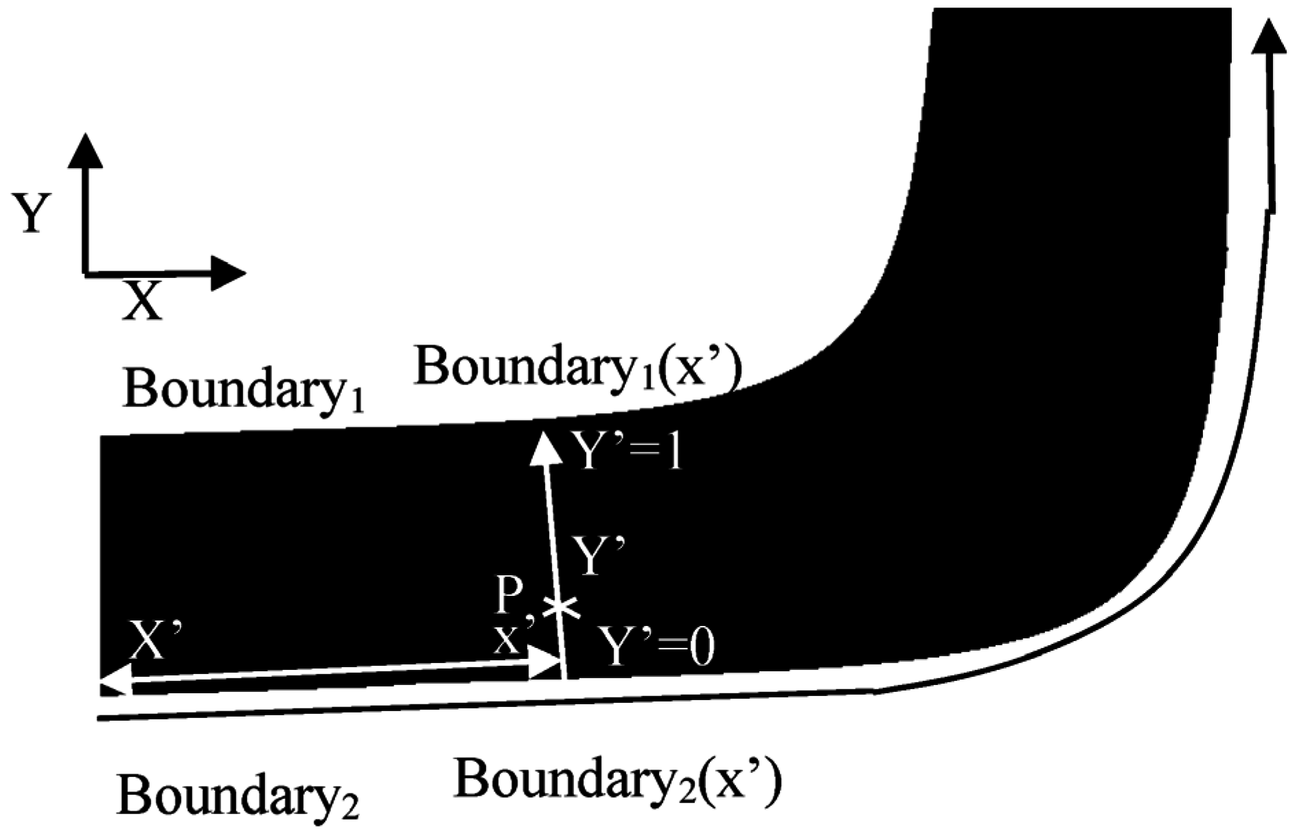Whilst this is an extensive assumption, it is possible with modern technology, with sensors, such as 3D LiDAR, ultrasonics, arrays of 3D vision cameras with advances in computer vision, etc. The possibility of having multiple intelligent vehicles in the vicinity also allows for the sharing of vision information across vehicles to rectify errors and give information about occluded areas. The algorithm used a road coordinate axis system along with the Cartesian coordinate axis system. The road coordinate axis system (X’Y’) employed the X’ axis as Boundary₂ and the Y’ axis as the ratio of the distance of the present point of the vehicle from Boundary₂, as compared to the overall road width. The representation of any point P(x,y) could hence be given by Equation (1), and the terms are explained by Figure 1.

$$P(x,y)=P(x\prime ,y\prime )=P\left(x\prime ,\frac{\Vert P(x,y)-Boundar{y}_2(x\prime )\Vert }{\Vert Boundar{y}_1(x\prime )-Boundar{y}_2(x\prime )\Vert }\right)$$

(1)

Figure 1. Road and Cartesian coordinate axis system [12].

Figure 1. Road and Cartesian coordinate axis system [12].

The algorithm enabled planning and moving a vehicle, so that the separation available from the vehicle on all sides was larger than separMin_i. This was referred to as the aggression factor. The notion was to always keep as large a separation as possible, which meant greater safety; however, the attempt to maximize separation was subject to a threshold of separMax_i. Higher values of the factor encouraged vehicles to make driving decisions, such that very high separation from other vehicles was very likely, while a low value of the factor encouraged aggressive driving decisions, such as close overtaking, wherein separations from other vehicles was likely to be very low. The solution was modelled as a set of behaviours. Each behaviour had a set of preconditions that had to be met for the particular behaviour to be initiated. The following is the complete list of behaviours:

• Obstacle avoidance: Obstacle avoidance behaviour is called whenever any obstacle or set of obstacles are sensed on the road. The vehicle attempts to overcome each obstacle by the widest possible margin (under a maximum of separMax_i).
• Centring: In the case that the vehicle does not find any obstacle or any other vehicle in the scenario, the vehicle slowly drifts towards the centre of the road.
• Lane change: Whenever any vehicle makes a lateral change on the road, the change carries the risk of an accident with any vehicle to the rear, which may be travelling at a higher speed and may now suddenly find that the vehicle in question has cut-in ahead of it. Hence, all behaviours involving changing of lateral positions are checked, and only those behaviours that ensure that all vehicles would have enough time to adjust their speeds are allowed, if the lane change behaviour actually proceeds.
• Overtaking: If a faster vehicle sees a slower vehicle directly ahead, which restricts its motion, it may attempt to overtake the slower vehicle. Overtaking can be direct or indirect. In direct overtaking, enough separation is available (along with the minimum safety distance) on either side of the slower vehicle, for overtaking to be initiated. If both sides can host the overtaking, the easier side is chosen. In indirect overtaking, enough separation is not initially available, but can be made available if the entire stream of vehicles ahead moves laterally on the road. Indentation.
• Be overtaken: If a slower vehicle ahead sees a faster vehicle behind trying to overtake, it may need to cooperate to give some additional separation to enable the overtaking to occur safely. The slower vehicle firstly assesses the side by which the overtaking is being attempted and then computes the distance by which it must laterally move.
• Maintain separation steer: This behaviour attempts to maximize the immediate separation available between the vehicle and any other entity, if the immediate separation on either side is less than the maximum threshold of separMax_i.
• Slow down: If the vehicle cannot maintain the minimum separation of separMin_i on both sides, it is taken as a risk, and the vehicle is required to slow down.
• Discover conflicting interests: If two vehicles are seen to be steering towards each other because of any behaviours, there is clearly a potential risk. Once it is evident that a minimum threshold separation would be crossed, the trajectories of travel of the vehicles are straightened.
• Travel straight: The vehicle is simply asked to travel straight ahead, keeping itself aligned parallel to the road edges.

4. Single-Lane Overtaking

For this problem, it is assumed that the road is marked in the middle by a real or virtual boundary separating the outbound and incoming directions of travel. The behaviours introduced in Section 2 are all used, and their computations are done using this boundary. As a result, while driving using any of the behaviours, the vehicle does not slip into the wrong side of the road at all, even though there may be no physical barrier separating the sides. The single-lane overtaking behaviour is modelled in addition to these behaviours. The computation of the single-lane behaviour, however, uses the actual road boundaries. Various aspects of the behaviour are detailed as follows.

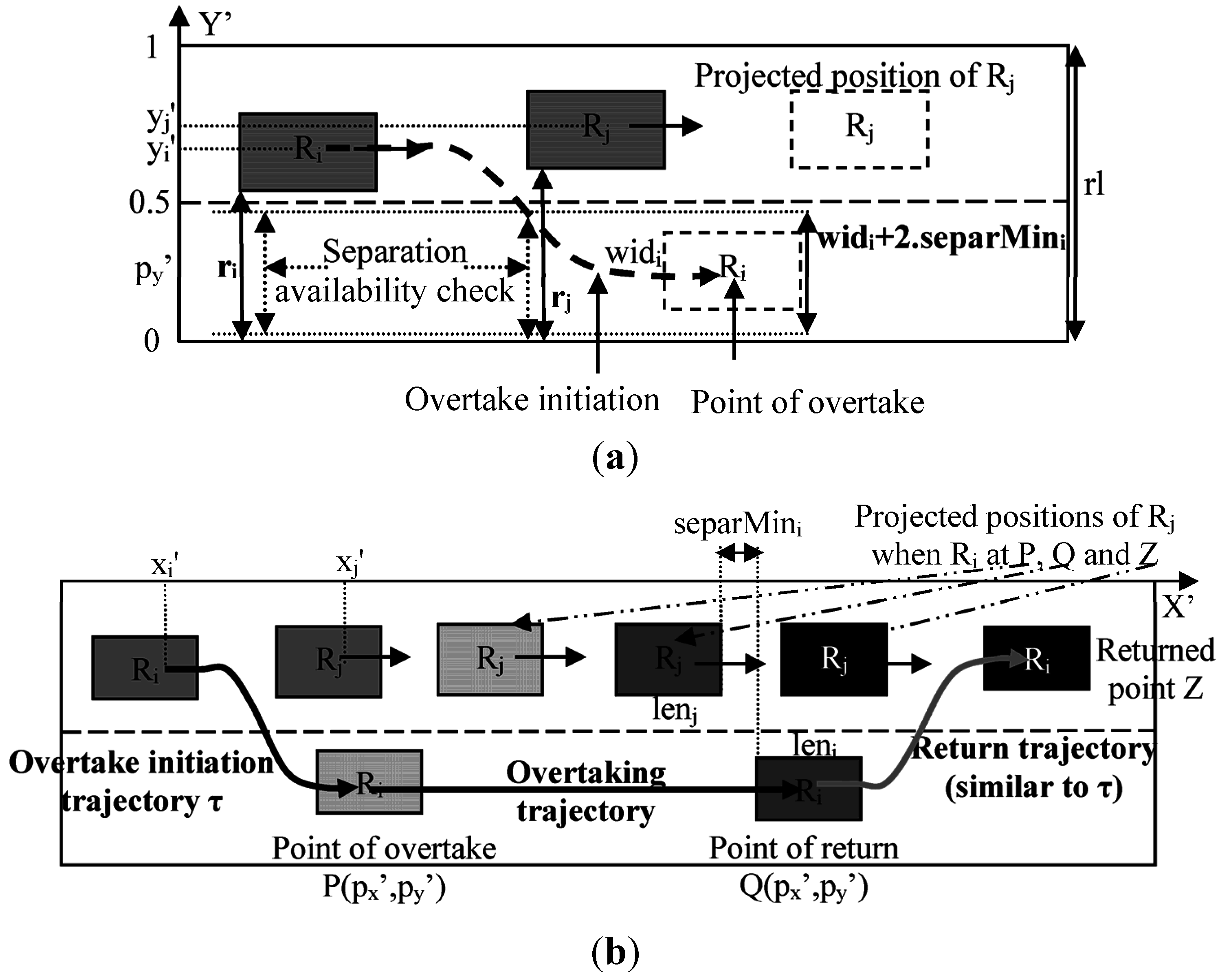
4.1. Single-Lane Overtaking Initiation

Consider that the vehicle being planned R_i cannot overtake a slower vehicle in front by normal means. It may attempt to see if single-lane overtaking is possible. It is required that the vehicle is currently on the correct side of the road and not already attempting single-lane overtaking. As per the general methodology of overtaking trajectory computation, we need to firstly decide whether the overtaking will happen on the left side or right side of the vehicle ahead and then select the preferred lateral position for overtaking. Here, it is assumed that the traffic operates with a “drive on the left” rule, and hence, single-lane overtaking can only happen on the right side.

Consider that the vehicle in front is R_j with a separation of r_j available on its right (without considering the virtual boundary). Furthermore, consider that the vehicle R_i has a separation r_i on its right side. The availability of these separations may be partly on the correct (outbound) carriageway and partly on the wrong (inbound) carriageway. The most important precondition for the overtaking to be initiated is that both of these separations must be larger than the minimum separation required by R_i for it to overtake, which is its width (wid_i) and a safety distance (separMin_i) on both sides, totalling wid_i + 2.separMin_i. The notations are shown in Figure 2a.

Figure 2. Notations used in single-lane overtaking. (a): For overtaking initiation; (b): Completion of overtaking.

Figure 2. Notations used in single-lane overtaking. (a): For overtaking initiation; (b): Completion of overtaking.

On availability of the separation, the next task is computing a point P(p_x’,p_y’) to which the vehicle may travel for overtaking to occur. Usually, this overtaking point would lie on the wrong side of the road. On reaching P(p_x’,p_y’), the vehicle may travel almost straight ahead to move in front of the vehicle being overtaken and subsequently may attempt to return to the original lane. p_y’ denotes the lateral position that the vehicle attempts to achieve during the overtaking procedure. The basic requirement is separation maximization, and hence, this point must be far enough from the vehicle being overtaken, as well as from any other vehicle or road boundary that may lie towards the right. The maximization is under a threshold of separMax_i which disallows the vehicle from going too far on a wide road that would require large steering movements. Computation of p_y’ is given by Equation (2).

$$p_y^{\prime }=\{\begin{array}{ccc}\begin{array}{c}(y_j^{\prime }.rl-wi{d}_j/2-separMa{x}_i-wi{d}_i/2)/rl\\ (y_j^{\prime }.rl-wi{d}_j/2-r_j/2)/rl\end{array}& \begin{array}{c}{r}_j\ge wi{d}_i+2separMa{x}_i\\ r_j<wi{d}_i+2separMa{x}_i\end{array}& \begin{array}{c}(i)\\ (ii)\end{array}\end{array}$$

(2)

Here, rl is the current width of the road and y_j’ is the position of R_j in the Y’ axis. Equation 2(i) denotes the condition when the separation available on the right of R_j is wide enough for the vehicle R_i to enjoy a maximum separation of separMax_i on both sides. Equation 2(ii) denotes the condition when the largest possible separation is not available, and hence, R_i simply attempts to drive in between the separation available.

The value of p_x’ is the same as per the general guidelines used in [12], given by Equation (3). The basic idea is that the curve generated for the travel of the vehicle till the point of overtake P(p_x’,p_y’) must be smooth enough for navigation with the current speed v_i.

p_x’ = c₁ + c₂.v_i + c₃. abs(y_i’ − p_y’).rl

(3)

Here, c₁, c₂, c₃ are constants, abs() is the absolute value function and y_i’ is the current position of R_i in the Y’ axis. c₁ is the minimum distance on the X’ axis needed to produce a smooth curve as per spline curves. Cubic splines are used with the constraint that the spline must start from the current position, headed in the current orientation of the vehicle, and should end at the point of overtake headed parallel to the road. Usually, this is set to be twice the length of the vehicle. c₂ and c₃ meanwhile denote the contributions of the factors of speed and steering requirements. Spline curves are used to compute the overtaking initiation trajectory τ from the current vehicle position R_i to P(p_x’,p_y’), such that the vehicle is parallel to the road at P(p_x’,p_y’).

The time required for the vehicle to place itself in the overtaking zone is given by ||τ||/v_i, where ||τ|| is the length of the trajectory and v_i is the current vehicle speed. The vehicle may then be seen to accelerate from its original speed v_i to the maximum speed vMax_i in order to be well ahead of R_j (with an additional safety distance of separMin_i) before its return to the correct side can take place. In normal circumstances, the trajectory for the vehicle to return to the correct side of the road is similar (flipped) to the overtaking trajectory. However, its speed will have increased to vMax_i, giving a return time of ||τ||/vMax_i, which will be shorter than ||τ||/v_i. Overall, we can then find the total overtaking period with the corresponding expected straight trajectory, called the overtaking trajectory. The notations are shown in Figure 2b. The total time for overtaking may hence be approximated by Equation (4).

$$T=\frac{\Vert \tau \Vert }{v_i}+\frac{x_j^{\prime }-x+_i^{\prime }\max \left(le{n}_i,le{n}_j\right)/2+separMi{n}_i}{\frac{v_i+vMa{x}_i}{2}-v_j}+\frac{\Vert \tau \Vert }{vMa{x}_i}$$

(4)

Here, x_i’ and x_j’ denote the current position of R_i and R_j, respectively, while len_i and len_j denote the corresponding lengths. v_j is the current speed of R_j.

For single-lane overtaking to be initiated, the preconditions of the general overtaking behaviour (Section 2) are included, that is the lane change behaviour (Section 2) for trajectory τ must be true, as well as the condition that R_j must not be drifting rightward. Further, no collisions should occur between the vehicle R_i and any other vehicle (as per their projected travel) on the wrong side of the road, if R_i occupies the computed lateral position for the time interval T. This means, ideally, if the vehicles stick to their current speeds and lateral positions, the vehicle R_i should be able to complete the overtaking procedure within time T without causing any vehicles to slow down.

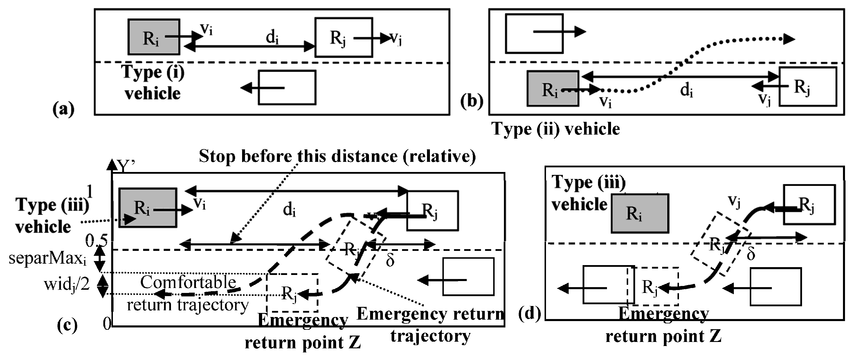
4.2. General Travel

In case a vehicle is travelling on the wrong side of the road and wishes to attempt single-lane overtaking, it must always test whether such overtaking is feasible or whether it has been completed, which are modelled as separate behaviours and discussed in Sections 4.3 and Sections 4.4. In all other cases, the vehicle must travel in the wrong lane using the same behaviour set as any general vehicle (travelling on the correct side of the road), with the exception that no overtaking can be performed. This would mean that mostly either the vehicle travels straight ahead or adjusts its lateral position to maximize its separation from all other vehicles.

The speed needs to be set for every vehicle in the planning scenario whilst it travels during single-lane overtaking or any other behaviour. As per the heuristics used, each vehicle must always attempt to travel within its maximum safe speed. This notion is, however, different for the different classes of vehicles possible.

The first type of vehicle (i) is a normal vehicle, which is on its correct side of travel, and no other vehicle attempting single-lane overtaking is to be found ahead (Figure 3a). For such a vehicle, it is assumed that in the worst case, the vehicle driving in front might brake suddenly, and hence, the speed should correct to enable the vehicle to react instantaneously and avoid a collision with a safety distance of separMin_i. The preferred speed is given by Equation (7(i)).

Figure 3. Various types of vehicles and notations for their speed computation.

Figure 3. Various types of vehicles and notations for their speed computation.

The second category of vehicle (ii) is one which is on the wrong side of the road in the middle of attempting single-lane overtaking and finds a vehicle R_j directly ahead of it (Figure 3b). Hence, R_i and R_j are travelling towards each other with speeds v_i and v_j. The attempt here is to stop R_i, which is the vehicle being planned, before a possible collision. The speed must always be such to enable R_i to stop with the maximum possible deceleration. The speed setting is hence the same as for a normal vehicle, with the resultant safe speed interpreted as the resultant safe relative speed. The preferred speed is given by Equation (7(ii)).

The last category (iii) is if the vehicle R_i is on the correct side of the road with vehicle R_j travelling towards it on the wrong side, attempting single-lane overtaking (Figure 3c). Vehicle R_i is aware of the fact that R_j needs to travel back to its correct side, and hence, mere collision prevention is not enough. If R_i and R_j stand almost touching each other, neither can move until one of the vehicles backs up. R_j needs some distance to return to its correct side. In an extreme case, R_j should have additional space available to steer left and return to its correct lane (Figure 3d) using an emergency return trajectory, while still avoiding collision with R_i. R_j would need to stop and wait for the other vehicles to clear on the correct side and slowly trace the emergency return trajectory. In extreme cases, both the vehicles R_i and R_j should slow down sufficiently for R_j to return. This additional distance was not maintained by the earlier category (or R_j itself does not contribute much in slowing down), as it is important for R_j to get close to R_i while tracing the emergency return trajectory. R_j must return to the correct side and not stop because of the presence of R_i. Otherwise, both vehicles may wait indefinitely.

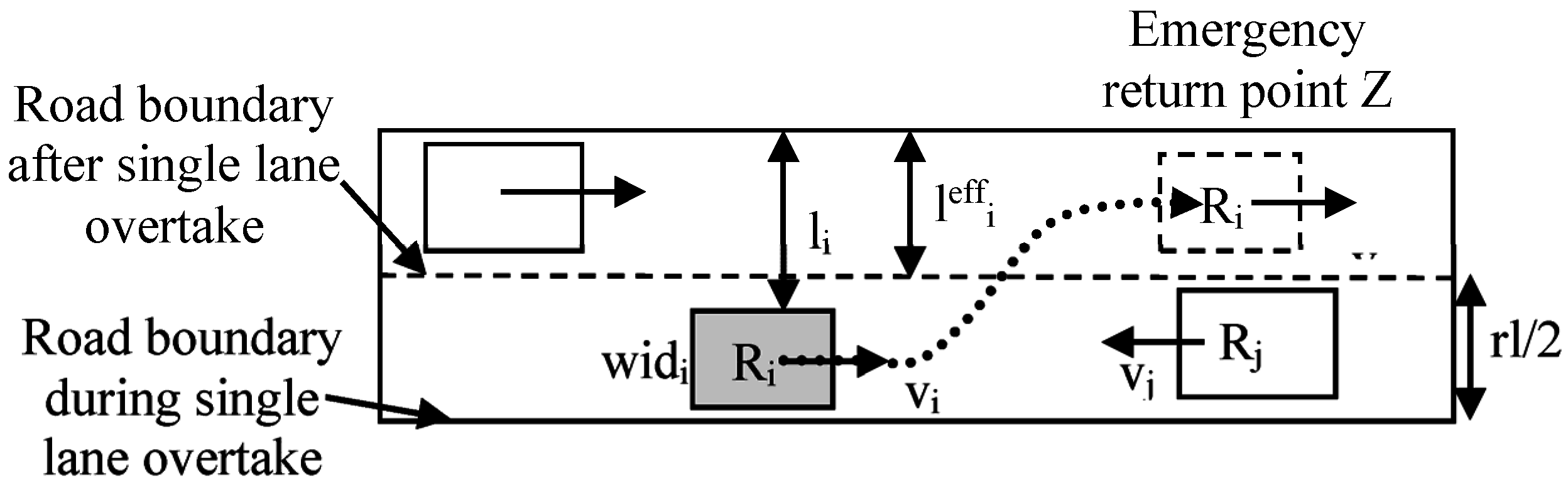
As perceived by R_i, if the vehicle R_j immediately needs to return to its original lane, it would need to choose an emergency point of return Z(z_x’,z_y’). Here, z_y’ is the chosen lateral position to which R_j would return. Assuming sufficient distance would be available with R_j, its lateral position at the return can be given by Equation (5). Y’ = 0.5 is the virtual boundary from which the maximum separation distance is desired.

$$z_y^{\prime }=0.5+\left(wi{d}_j/2+separMa{x}_i\right)/rl$$

(5)

The distance required (δ) along the road to change the lateral position as computed in Equation (5) is given by Equation (6), whose notations are the same as those in Equation (3). It is assumed here that half of this distance would be required on the wrong side of the road, while the other half would be on the correct side of the road, and hence, only the first half is in question. This is shown clearly in Figure 4.

δ = (c₁ + c₂.v_i + c₃. Abs(y’ – z_y’).rl)/2

(6)

The vehicle R_i attempts to change its speed such that this distance can be assured even if R_i has to stop to make this distance available. The relative speed is computed, which is used to compute the actual speed given by Equation (7(iii)).

The preferred speeds for various cases are given by Equation (7), while the actual speeds considering acceleration limits are given by Equation (8). Here, d_i is the distance of R_i from the vehicle or obstacle in front.

$$vm=\{\begin{array}{cc}\begin{array}{c}\sqrt{2.accMa{x}_i.\max \left(d_i-separMi{n}_i,0\right)}\\ \max \left(\sqrt{2.accMa{x}_i.\max \left(d_i-separMi{n}_i,0\right)}-v_j,0\right)\\ \max \left(\sqrt{2.accMa{x}_i.\max \left(d_i-separMi{n}_i-\delta ,0\right)}-v_j,0\right)\end{array}& \begin{array}{c}(i)\\ (ii)\\ (iii)\end{array}\end{array}$$

(7)

$$v_i^{\prime }=\{\begin{array}{cc}\begin{array}{c}\min (v_i+accMa{x}_i,v_i^{\max })\\ \max (v_i-accMa{x}_i,vm)\\ vm\end{array}& \begin{array}{c}{v}_i+accMa{x}_i\le v_m\\ v_i>v_m\\ otherwise\end{array}\end{array}$$

(8)

Figure 4. Return point calculation.

Figure 4. Return point calculation.

4.3. Cancelling Single-Lane Overtaking

While a vehicle R_i is attempting single-lane overtaking, factors unaccounted for in its initiation may stop the overtaking from being successfully completed, and the vehicle may need to return to its original side as quickly as possible. Driving on the wrong side is dangerous and creates problem for the entire traffic system. Hence, the feasibility of overtaking must be continuously tracked during the whole overtaking process. At any time, overtaking may be regarded as infeasible if there is some vehicle R_j in front, driving towards R_i and the distance between the two vehicles is just large enough (or below) the minimal distance required by R_i to execute the emergency return trajectory. This minimum distance (δ) is given by Equation (6). If the current distance is just equal or less than the required amount or R_i cannot decelerate fast enough to stop the distance (δ) from reducing below this amount, single-lane overtaking is regarded as being cancelled on that occasion.

The vehicle now needs to actually return to its original side of travel. In this stage, the actual point of emergency return Z(z_x’,z_y’) is computed by an analysis of the vehicles on the correct side. Suppose l_i is the separation to the left that is currently available. This distance does not account for the fact that after R_i returns to its lane, the virtual boundary would become the boundary to keep away from, and hence, the effective distance available to the left is that beyond the virtual boundary given by Equation (9). The notations are shown in Figure 4.

l^eff_i = l_i − (rl/2 − y^’_i.rl − wid_i/2)

(9)

Based on the guidelines of separation maximization under a threshold of separMax_i, the desired lateral position of the vehicle is given by Equation (10). In case the minimum separation is not available, R_i needs to attempt to return back to the correct side whilst maintaining at least a minimum separation.

$$Z_y^{\prime }=\{\begin{array}{cc}\begin{array}{c}0.5+\left(wi{d}_j/2+separMi{n}_i\right)/rl\\ 0.5+\left(wi{d}_j/2+separMa{x}_i\right)/rl\\ 0.5+l_i^{eff}/2.rl\end{array}& \begin{array}{c}{l}_i^{eff}\le wi{d}_i+2.separMi{n}_i\\ l_i^{eff}\ge wi{d}_i+2.separMa{x}_i\\ wi{d}_i+2.separMa{x}_i<l_i^{eff}<wi{d}_i+2.separMa{x}_i\end{array}\end{array}$$

(10)

The (emergency) return trajectory τ is computed using spline curves joining the current point to the point of return Z. The trajectory is traversed at all times with the highest possible speeds as calculated in Equation (8). Since the return trajectory might not be clear, it is evident that the vehicle may have to slow down drastically and even stop and wait for some vehicles to clear. However, it would eventually return to its original side.

4.4. Completing Single-Lane Overtaking

Once R_i, which was attempting single-lane overtaking, is ahead of the vehicle being overtaken, it may aim to return to its original side of travel. This behaviour is in fact the same as cancelling the single-lane overtaking behaviour with the exception that it is invoked post overtaking and only when the minimum separation is available. In the absence of minimum separation, the vehicle continues to traverse on the wrong side of the road. It may return when the minimum separation is available or may be forced to return by cancellation of the single-lane overtaking behaviour when a vehicle in front, travelling in the opposite direction, is too near. Implementation details are then the same as for the cancelling single-lane overtaking behaviour.

The resultant set of behaviours is summarized in Table 1, and the resultant algorithm is given as Algorithm 1. Table 1 and Algorithm 1 are extended from [12].

Algorithm 1:

Plan (Vehicle Ri, Map, Previous plan τ)

If new obstacle found Compute τ for obstacle avoidance If lane_change (τ), return τ Else, vi ← max (vi—accMaxi,0), Ri ← move a unit step, return null

If no slower vehicle and obstacle ahead in vicinity $\wedge$ vi close to vimax $\wedge$ τ = null CEN ← (xi' + Δ(vi), 0.5) τ ← curve (Ri,CEN) If τ(t) $\in$ ζifree $\forall$ t, return τ

If τ ≠ null vi ← Safe speed as per Equation (8) If Conflicting Interests $\wedge$ τ is non-straight τ ← straighten(τ), return τ Else If performing single-lane overtake Calculate δ using Equation (6) If distance δ not available or not expected to be available in the future even with largest deceleration Compute Z for return using Equation (10) τ ← curve (Ri,Z)    return τ Else   Ri ← Move a unit step by τ   If τ is over, return null, else return τ

Else If performing single-lane overtake Calculate δ using Equation (6) If distance δ not available or not expected to be available in the future even with largest deceleration Compute Z for return using Equation (10) τ ← curve(Ri,Z)   return τ

If slow vehicle in front ˄ sufficient separation exists for overtaking assuming cooperation ˄ not undergoing single-lane overtake Rj ← Vehicle to overtake, side ← side of overtaking Compute P for overtake τ ← curve(Ri,P) If τ(t) $\in$ ζifree $\forall$ t $\wedge$ lane_change(τ) $\wedge$ Rj not steering towards side,    return τ

If Slower vehicle in front $\wedge$ sufficient separation available $\wedge$ no collisions with vehicle in wrong side for expected time of completion of overtake assuming no cooperation Rj ← Vehicle to overtake Compute P for single-lane overtake using Equations (2) and (3) τ ← curve(Ri,P) Calculate T by Equation (4) If τ(t) $\in$ ζifree $\forall$ t $\wedge$ lane_change(τ) $\wedge$ no collisions with vehicles in wrong side till T assuming no cooperation $\wedge$ Rj not steering towards side   return τ

If performing single-lane overtake $\wedge$ sufficient separation available at correct side Compute Z for return using Equation (10) τ ← curve(Ri,Z) If τ(t) $\in$ ζifree $\forall$ t $\wedge$ lane_change(τ), return τ

If vehicle overtaking at back $\wedge$ separation available to offer $\wedge$ not undergoing single-lane overtake Rj ← Vehicle to allow overtake, side ← side of being overtaking Compute P for being overtaken τ ← curve(Ri,P) If τ(t) $\in$ ζifree $\forall$ t $\wedge$ lane_change(τ), return τ

If li + ri ≥ 2.min_separi ˄ (li <max_separi ˄ ri < max_separi) Compute P for separation maintenance τ ← curve(Ri,P) If τ(t) $\in$ ζifree $\forall$ t $\wedge$ lane_change(τ), return τ

If li + ri < 2.min_separi vi ← max(vi—accMaxi,0), Ri ← move a unit step, return null vi ← Safe speed as per Equation (8) Ri ← Move a unit step parallel to the road return null

Table 1. Summary of vehicle behaviours.

S. No.	Behaviour	Pre-Condition	Description	In-Behaviour Specifications	Priority
1.	Obstacle avoidance	Obstacle discovery, lane change true	Strategy to avoid obstacle	Check for collisions with vehicle in front, obstacle avoidance	1
2.	Centring	No vehicle, no obstacle, vehicle travelling at high speed	Put vehicle in the centre of the road	NIL	2
3.	Lane change	Called by other behaviours	Whether possible to steer	NIL	NA
4.	Overtake	Slower vehicle ahead, sufficient separation available assuming the cooperation of all vehicles ahead, lane change true, not undergoing single-lane overtaking	Strategy to initiate overtaking, ask other vehicles to move and eventually align, so that travelling straight completes overtaking	Discover conflicting interests, check for collisions with vehicles in front	3
5.	Single-lane overtaking	Slower vehicle ahead, sufficient separation available, lane change true, no collisions with a vehicle on the wrong side for the expected time of completion of overtaking assuming no cooperation	Attempt to initiate single-lane overtaking by placing the vehicle on the wrong side	Check for cancellation of single-lane overtaking, check for collision with vehicle in front	4
6.	Cancel single-lane overtaking	Performing single-lane overtaking, sufficient separation not available or not expected to be available in the future even with the largest deceleration to return to the original lane because of a vehicle ahead on the wrong side	Attempt to place the vehicle on the correct side and not allow any subsequent motion on the wrong side	Check for collision with the vehicle in front and if clear move ahead	NA
7.	Complete single lane overtaking	Performing single-lane overtaking, sufficient separation available on the correct side, lane change true	After completing overtaking, return to the correct side	Check for collision with the vehicle in front	5
8.	Be overtaken	Vehicle to the rear shows the need for overtaking, separation available to offer, lane change true, not undergoing single-lane overtaking	Align so that the vehicle to the rear needing to overtake has more overtaking separation	Discover conflicting interests, check for collisions with the vehicle in front	6
9.	Maintain separation steer	Maximum separation possible not available at both ends, while steering in some manner can increase current lowest separation, lane change true	Steer to maintain as high separation as possible (not more than threshold) from both ends	Discover conflicting interests, check for collision with vehicle in front	7
10.	Slow down	No adjustment of steering capable of generating minimal separation at both ends	Reduce speed	NIL	8
11.	Discover conflicting interests	A neighbouring vehicle steering towards vehicle being planned found too close while the vehicle being planned was steering towards it, vehicle following a non-straight trajectory	Straighten trajectory being followed	Check for collision with the vehicle in front	NA
12.	Travel straight	No pre-conditions	Take a unit step forward as per the road’s current orientation	Check for collisions with the vehicle in front	9

Table 1. Summary of vehicle behaviours.

S. No.	Behaviour	Pre-Condition	Description	In-Behaviour Specifications	Priority
1.	Obstacle avoidance	Obstacle discovery, lane change true	Strategy to avoid obstacle	Check for collisions with vehicle in front, obstacle avoidance	1
2.	Centring	No vehicle, no obstacle, vehicle travelling at high speed	Put vehicle in the centre of the road	NIL	2
3.	Lane change	Called by other behaviours	Whether possible to steer	NIL	NA
4.	Overtake	Slower vehicle ahead, sufficient separation available assuming the cooperation of all vehicles ahead, lane change true, not undergoing single-lane overtaking	Strategy to initiate overtaking, ask other vehicles to move and eventually align, so that travelling straight completes overtaking	Discover conflicting interests, check for collisions with vehicles in front	3
5.	Single-lane overtaking	Slower vehicle ahead, sufficient separation available, lane change true, no collisions with a vehicle on the wrong side for the expected time of completion of overtaking assuming no cooperation	Attempt to initiate single-lane overtaking by placing the vehicle on the wrong side	Check for cancellation of single-lane overtaking, check for collision with vehicle in front	4
6.	Cancel single-lane overtaking	Performing single-lane overtaking, sufficient separation not available or not expected to be available in the future even with the largest deceleration to return to the original lane because of a vehicle ahead on the wrong side	Attempt to place the vehicle on the correct side and not allow any subsequent motion on the wrong side	Check for collision with the vehicle in front and if clear move ahead	NA
7.	Complete single lane overtaking	Performing single-lane overtaking, sufficient separation available on the correct side, lane change true	After completing overtaking, return to the correct side	Check for collision with the vehicle in front	5
8.	Be overtaken	Vehicle to the rear shows the need for overtaking, separation available to offer, lane change true, not undergoing single-lane overtaking	Align so that the vehicle to the rear needing to overtake has more overtaking separation	Discover conflicting interests, check for collisions with the vehicle in front	6
9.	Maintain separation steer	Maximum separation possible not available at both ends, while steering in some manner can increase current lowest separation, lane change true	Steer to maintain as high separation as possible (not more than threshold) from both ends	Discover conflicting interests, check for collision with vehicle in front	7
10.	Slow down	No adjustment of steering capable of generating minimal separation at both ends	Reduce speed	NIL	8
11.	Discover conflicting interests	A neighbouring vehicle steering towards vehicle being planned found too close while the vehicle being planned was steering towards it, vehicle following a non-straight trajectory	Straighten trajectory being followed	Check for collision with the vehicle in front	NA
12.	Travel straight	No pre-conditions	Take a unit step forward as per the road’s current orientation	Check for collisions with the vehicle in front	9

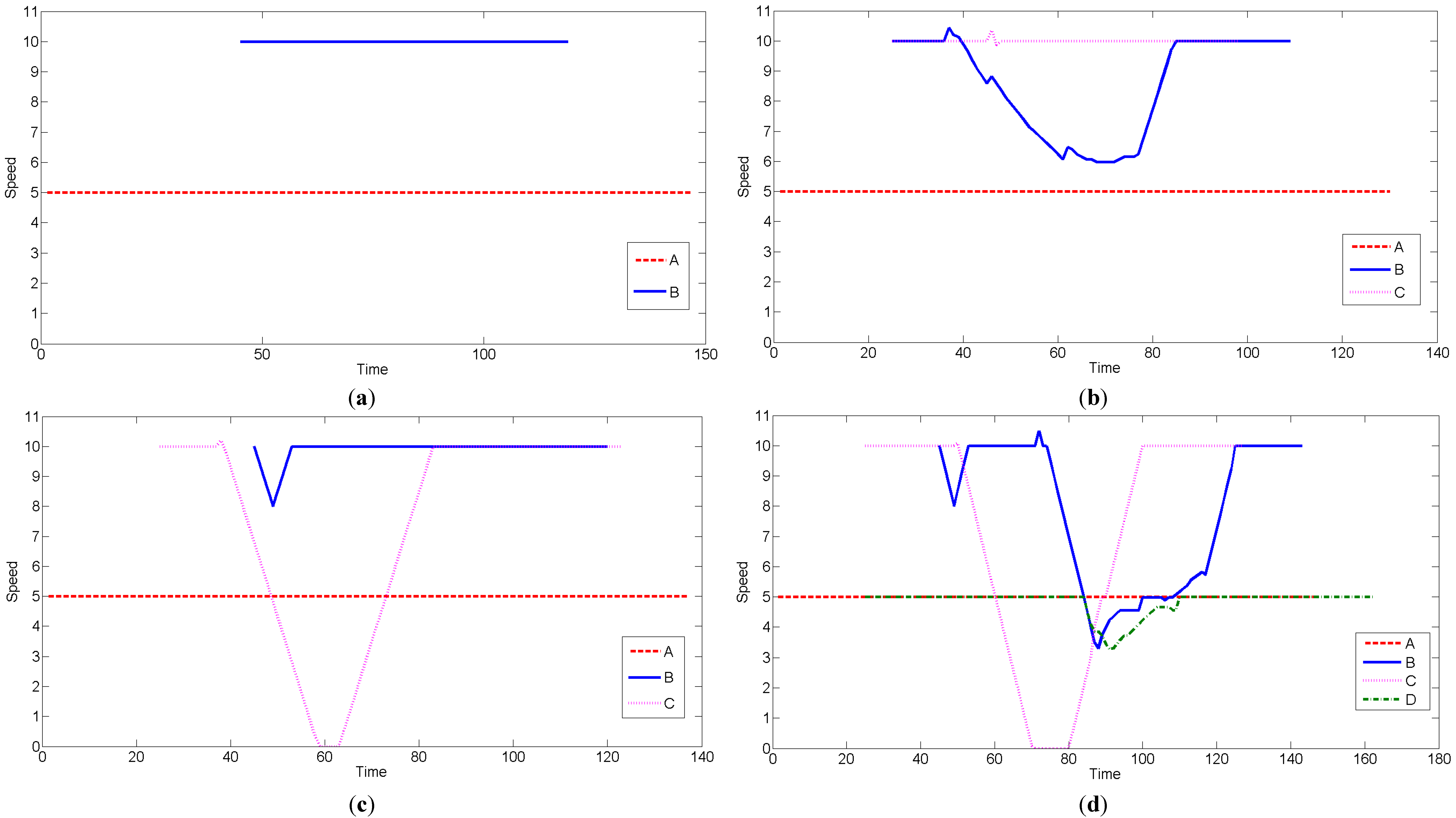
5. Results

The designed set of behaviours was studied via a series of simulations. The road considered was wide enough for only two vehicles to be accommodated comfortably. Half the width was reserved for traffic travelling in one (outbound) direction and the other half for traffic travelling in the other (inbound) direction. This is the most typical and the only likely scenario where such overtaking would take place. Indeed, wider roads may not necessitate that traffic from both directions mixes with each other. Different scenarios involving a single-lane overtaking were tested.

Being a very risky behaviour, most of the time, single-lane overtaking would not be attempted. Hence while we looked at many scenarios with numerous vehicles, most of them showcased no single-lane overtaking behaviour. The performance of vehicles without this behaviour was the objective of our previous work [12] and is hence not repeated in the current work. This can be practically seen in everyday life, as such overtaking is rarely seen and, then, only too when the conditions are the most favourable or idealistic. The visual display of all single-lane overtaking behaviours was the same, and hence, those results are not displayed. We tried to put the most interesting or the closest overtaking cases in the paper, as the other results are much easier to obtain.

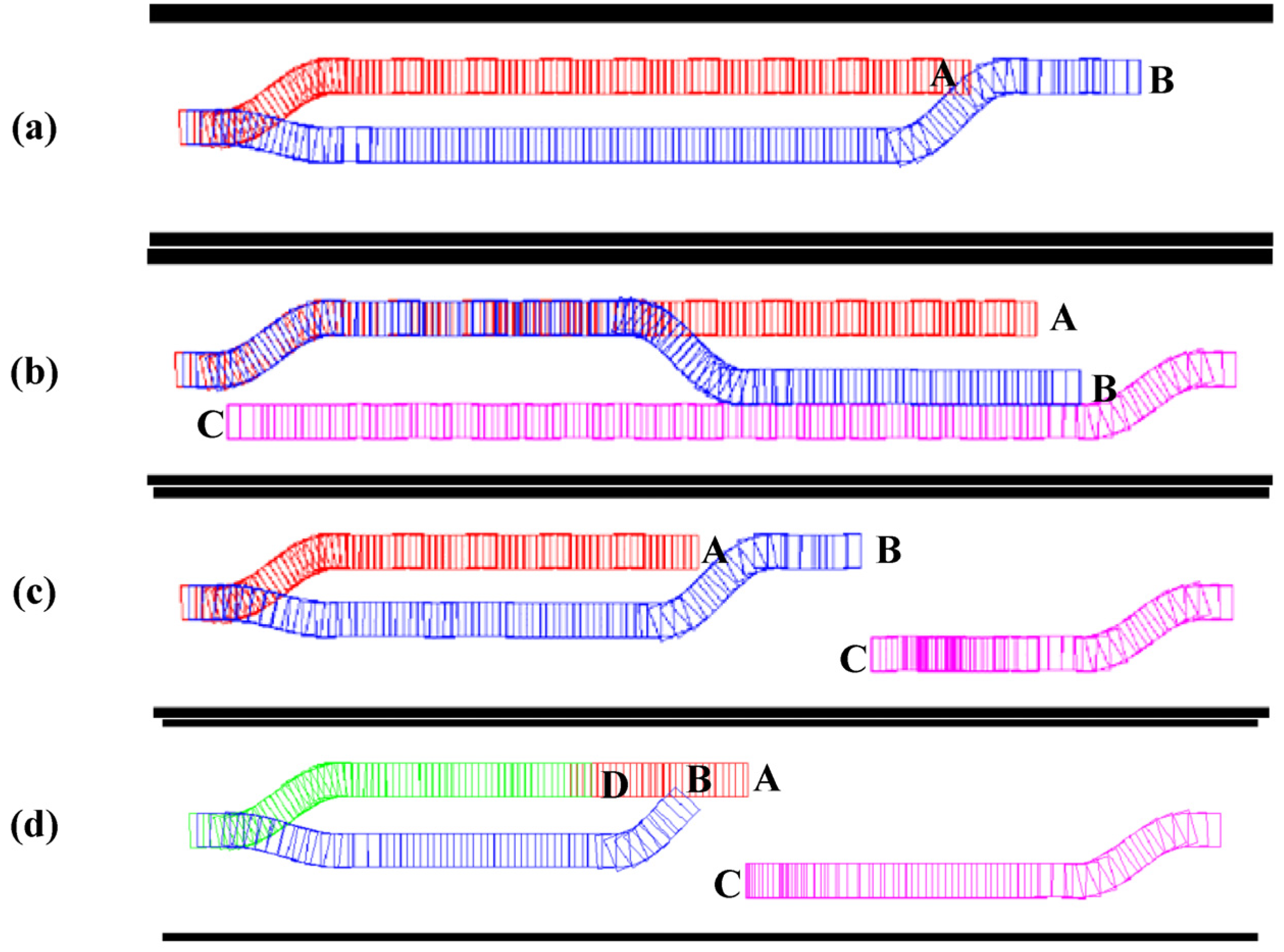
In the first scenario, a slower vehicle (A) was generated in the centre of the road, and this vehicle naturally simply drifted towards the correct side of travel. A faster vehicle (B) was generated later. The faster vehicle (B) judged the presence of the slower vehicle (A) ahead and the feasibility of single-lane overtaking. By the projected motion of B, it was clear that single-lane overtaking could easily happen by the vehicle going to the wrong side, and hence, the vehicle decided to perform single-lane overtaking. B jumps to the wrong lane or overtaking lane by the initiation of the single-lane overtaking behaviour, surpasses A by general travel during the single-lane overtaking behaviour and then decides to return back to the original lane by the completion of the single-lane overtaking behaviour. There was no change at all in the motion of A, and overtaking was easily completed as shown in Figure 5a and Video in supplementary information.

The second scenario was created to test the ability of a vehicle when such overtaking is not possible. In this scenario, an additional vehicle (C) was made to appear on the other side, travelling in the opposite direction. When the faster vehicle (B) emerged, it computed the feasibility of overtaking the slower vehicle (A) by considering the motions of A and C. C made single-lane overtaking seem risky, and hence, B did not attempt to overtake A. Instead, it followed A. When C had passed both A and B, again, the feasibility of single-lane overtaking was judged. This time, there was no vehicle that could make overtaking seem infeasible or risky. Single-lane overtaking by B was now judged to be feasible. It was initiated and subsequently completed in a manner similar to Scenario 1. The trajectories of the three vehicles and the scenario are shown in Figure 5b and Video in supplementary information.

In the third scenario, vehicle B judged single-lane overtaking to be feasible and initiated the same. There was, however, an oncoming vehicle (C) travelling on the other side of the road. The emergence and speed of C was just enough for overtaking to be feasible and just possible without cooperation. A slower speed for C would have made overtaking comfortable and, thus, not challenging, whereas a higher speed would have made overtaking infeasible. By fixing the speed of C in such a manner, the narrow overtaking behaviour was studied. On committing to overtaking, B quickly placed itself on the wrong side of the road, went ahead of the vehicle being overtaken (A) and returned in front of A in the correct lane. However, C was driving towards B during single-lane overtaking, which could have been a threat. C assessed a possible threat in advance by computing the relative speeds of the vehicles as a part of its normal driving behaviour and showed cooperation to some extent by slowing down. This gave A some extra space to return back to the correct side of the road and make overtaking comfortable and risk-free. The results are shown in Figure 5c and Video in supplementary information.

Figure 5. Experimental results. (a): Scenario 1—Simple single lane overtaking; (b): Scenario 2—Single lane overtaking with an oncoming vehicle; (c): Scenario 3—Single lane overtaking requiring the oncoming vehicle to slow down; (d): Scenario 4—Cancelling of single lane overtaking due to infeasibility by an oncoming vehicle.

Figure 5. Experimental results. (a): Scenario 1—Simple single lane overtaking; (b): Scenario 2—Single lane overtaking with an oncoming vehicle; (c): Scenario 3—Single lane overtaking requiring the oncoming vehicle to slow down; (d): Scenario 4—Cancelling of single lane overtaking due to infeasibility by an oncoming vehicle.

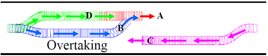
The aim in the last scenario was to put the overtaking vehicle (B) in an awkward scenario, which is the worst that such a vehicle can enter. The vehicle was made to initiate overtaking. In doing so, it did not account for A ahead, which would not allow B to return back to the correct lane easily on completion of single-lane overtaking. Overtaking was initiated, and the vehicle did go ahead of the slower vehicle D, with C coming from the other direction. After a little general driving on the wrong side of the road, it was clear that overtaking was not complete, because of the presence of A, and general driving could not continue, because C was approaching on the other side of the road. Hence, the infeasibility of overtaking was discovered, and an emergency return trajectory was computed. However, the emergency return trajectory was infeasible, due to a possible collision with A. C detected the infeasibility of B during its general driving speed assignment and slowed down to give enough space for B to eventually return back to its original side. B therefore placed itself in between the two slower vehicles (D and A). D saw B trying to accommodate during its general driving, and when B was able to slip in, D did well to give B accommodated in between. The scenarios are shown in Figure 5d and Video in supplementary information.

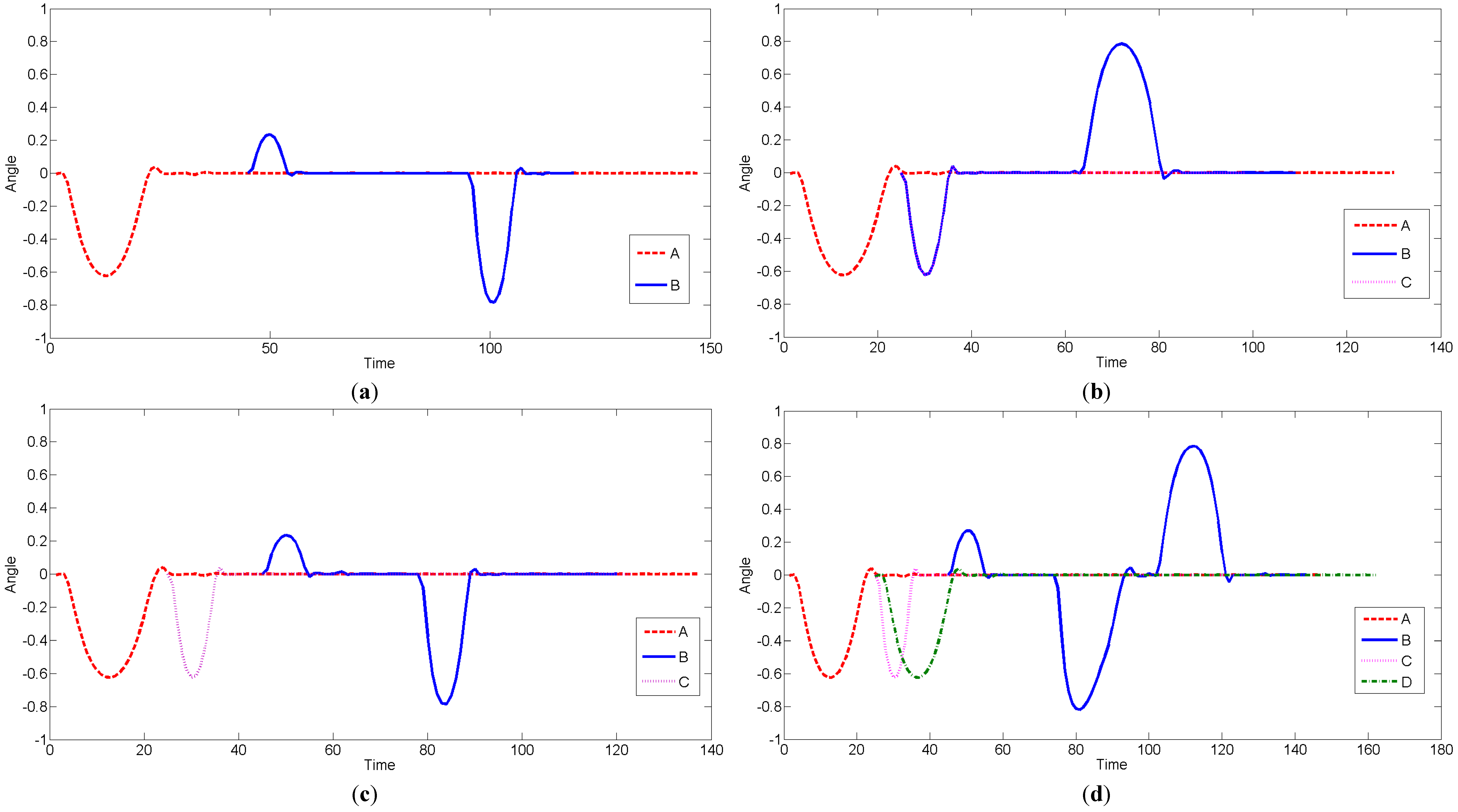
Figure 6. Angle profiles of different vehicles for different scenarios. (a): Scenario 1; (b): Scenario 2; (c): Scenario 3; (d): Scenario 4.

Figure 6. Angle profiles of different vehicles for different scenarios. (a): Scenario 1; (b): Scenario 2; (c): Scenario 3; (d): Scenario 4.

Figure 7. Speed profiles of different vehicles for different scenarios. (a): Scenario 1; (b): Scenario 2; (c): Scenario 3; (d): Scenario 4.

Figure 7. Speed profiles of different vehicles for different scenarios. (a): Scenario 1; (b): Scenario 2; (c): Scenario 3; (d): Scenario 4.

Table 2. Summarization of the results.

Scenario	Vehicle	Time to Destination	Distance Travelled till Termination	Maximum Allowed Speed	Average Speed
1.	A	147	716.2713	5	4.8726
	B	75	726.2893	10	9.6839
2.	A	130	632.2713	5	4.8636
	B	85	690.4683	10	8.1232
	C	74	716.1901	10	9.6782
3.	A	137	667.8519	5	4.8748
	B	76	730.2858	10	9.6090
	C	99	721.2544	10	7.2854
4.	A	147	716.2713	5	4.8726
	B	99	746.8892	10	7.5443
	C	103	714.8350	10	6.9401
	D	138	645.2713	5	4.6759

Table 2. Summarization of the results.

Scenario	Vehicle	Time to Destination	Distance Travelled till Termination	Maximum Allowed Speed	Average Speed
1.	A	147	716.2713	5	4.8726
	B	75	726.2893	10	9.6839
2.	A	130	632.2713	5	4.8636
	B	85	690.4683	10	8.1232
	C	74	716.1901	10	9.6782
3.	A	137	667.8519	5	4.8748
	B	76	730.2858	10	9.6090
	C	99	721.2544	10	7.2854
4.	A	147	716.2713	5	4.8726
	B	99	746.8892	10	7.5443
	C	103	714.8350	10	6.9401
	D	138	645.2713	5	4.6759

The statistical results relating to different scenarios are given in Table 2. Further, the angle and speed profiles for different vehicles are given in Figure 6 and Figure 7. In Figure 6a, both B and C turn towards their left simultaneously on entering the scenario, using similar dynamics. Hence, their angle profiles intersect. The units of distance and time are arbitrary and depend on the simulator. These can be mapped to real-world units by appropriate constants.

6. Conclusions

Enabling autonomous vehicles to drive in unorganized and chaotic traffic is a difficult problem that requires due consideration from a research perspective. In this paper, we made a significant step while considering traffic planning on straight roads as the specific problem being attacked. The work extended our earlier planning framework in which the assumption was that all vehicles were merely travelling on the same side of the road. By using the behaviours presented and experimented on in this paper, the framework can now be used in a variety of scenarios, both where roads are separated with a physical barrier or are just one-way and when the roads operate as a dual carriageway with no physical barrier. In particular, this paper looked in depth at the important overtaking procedure wherein a vehicle for some time occupies a part of the wrong side of the road in order to accomplish its overtaking activity. It is worth remembering that if such overtaking were not allowed, then the overall performance of the system would be much lower, with vehicles reaching their destination at a later time due to travelling for longer distances behind slower vehicles.

In the paper, we looked at aspects of assessing the feasibility of such overtaking and also at formulating an initiation trajectory, the mechanisms involved with driving on the wrong side, judging the infeasibility of such overtaking and cancelling and successfully completing an overtaking procedure. This behaviour was used in priority with the behaviours proposed earlier and practically meant that if normal overtaking, on the same side of the road, is not possible, then a vehicle would check for the possibility of single-lane overtaking.

Experimental evaluations were carried out by means of simulations. In particular, the single-lane overtaking behaviour was tested in various scenarios. In all cases, the vehicle either successfully completed the overtaking action or was able to cancel doing the same. No collisions were recorded using our method, and the vehicles apparently behaved in a similar fashion to actual vehicles on the road performing such overtaking. Currently, it is unfortunately neither possible to employ the algorithm on an actual vehicle and test it in real traffic, nor is it possible to verify such behaviour against standard traffic datasets. All traffic datasets are for organized traffic, while the work described here is for unorganized traffic. The difficulty of tracking vehicles in the absence of speed lanes makes obtaining such a dataset difficult. Having a dataset recording the motion of vehicles in real chaotic traffic would though enable the verification of the algorithm described here, as well as help to mine for new behaviours that could be used for planning. An autonomous vehicle requires different modules apart from planning, which need to be able to work in the absence of speed lanes. Clearly, these aspects can all be considered as future research.