
Polymorphic Clustering and Approximate Masking Framework for Fine-Grained Insect Image Classification


Information Engineering College, Henan University of Science and Technology, Luoyang 471000, China
*
Author to whom correspondence should be addressed.
Electronics 2024, 13(9), 1691; https://doi.org/10.3390/electronics13091691
Submission received: 11 March 2024
/
Revised: 13 April 2024
/
Accepted: 25 April 2024
/
Published: 27 April 2024
(This article belongs to the Special Issue Applications of Artificial Intelligence in Image and Video Processing)
Abstract
:Insect diversity monitoring is crucial for biological pest control in agriculture and forestry. Modern monitoring of insect species relies heavily on fine-grained image classification models. Fine-grained image classification faces challenges such as small inter-class differences and large intra-class variances, which are even more pronounced in insect scenes where insect species often exhibit significant morphological differences across multiple life stages. To address these challenges, we introduce segmentation and clustering operations into the image classification task and design a novel network model training framework for fine-grained classification of insect images using multi-modality clustering and approximate mask methods, named PCAM-Frame. In the first stage of the framework, we adopt the Polymorphic Clustering Module, and segmentation and clustering operations are employed to distinguish various morphologies of insects at different life stages, allowing the model to differentiate between samples at different life stages during training. The second stage consists of a feature extraction network, called Basenet, which can be any mainstream network that performs well in fine-grained image classification tasks, aiming to provide pre-classification confidence for the next stage. In the third stage, we apply the Approximate Masking Module to mask the common attention regions of the most likely classes and continuously adjust the convergence direction of the model during training using a Deviation Loss function. We apply PCAM-Frame with multiple classification networks as the Basenet in the second stage and conduct extensive experiments on the Insecta dataset of iNaturalist 2017 and IP102 dataset, achieving improvements of 2.2% and 1.4%, respectively. Generalization experiments on other fine-grained image classification datasets such as CUB200-2011 and Stanford Dogs also demonstrate positive effects. These experiments validate the pertinence and effectiveness of our framework PCAM-Frame in fine-grained image classification tasks under complex conditions, particularly in insect scenes.
1. Introduction
Fine-grained image classification (FGIC) involves the detailed classification of images belonging to the same broad category of objects. These objects include animals, plants, and artificial items, such as different species of birds [1], dogs [2], and insects [3,4], as well as individual instances of vehicles [5] and aircraft [6]. Fine-grained insect image classification is a subset of FGIC, focusing specifically on the next-level classification of insects.
There are over one million species within the insect class, distributed worldwide across various habitats and elevations, making them one of the most abundant animal groups on Earth playing crucial roles in ecosystems. Subcategories within the insect class exhibit extensive diversity, with some closely related species sharing similar visual characteristics in terms of color and texture. Traditional methods of insect classification often require field experts to conduct on-site collection and classification, which is costly and not suitable for large-scale scenarios. Low-cost fine-grained image classification tasks typically involve the use of cameras equipped with classification models placed at fixed locations or carried by drones to capture and classify images. However, the performance of such classification models is critical, alongside issues related to image quality. Therefore, employing an image classification model based on deep learning has emerged as a feasible approach to address fine-grained insect image classification problems.
Currently, the mainstream neural network models used in computer vision image classification are primarily divided into two categories: Convolutional Neural Networks (CNNs) [7] and Transformers [8]. CNNs excel at capturing local image features, while a Vision Transformer [9] from the visual field prioritizes capturing global image features through self-attention mechanisms, albeit with a weaker perception of local structures of the image. Both types of models have their own advantages and applicability, and the choice between them depends on the specific problem being addressed.
This paper mainly discusses and explores the fine-grained classification of insect images. The main experimental datasets include the Insecta subset of the iNaturalist 2017 dataset and the IP102 dataset. Some samples are shown in Figure 1.
The first row of Figure 1 shows insect image samples belonging to different categories that exhibit very similar visual appearances. The second row includes samples of two insect categories at different life stages, namely larva and adult. It can be seen that the visual difference of the samples in different life stages within the same category is significant, which is far more than the visual difference of different insects in the same life stage. Therefore, it is a challenge to accurately learn the classification characteristics of insect multi-life stages in fine-grained image classification of insect scenes. This raises two questions:
- How to accurately classify insect samples among easily confused approximate categories.
- How to accurately distinguish samples of the same insect category but at different life stages with significant visual differences.
There are few studies on fine-grained image classification tasks in the insect scene, and the targeted research on the above problems is currently missing. The mainstream networks in fine-grained image classification tasks in other scenarios, whether CNN or Transformer, represent the deep features of a single image itself, such as color, texture, and spatial relationship, into a tensor of some dimension. It is impossible to solve the non-horizontal relationship between each image (like the image of the same life stage and the image of the same different life stage should be used to extract category features and pay attention to the morphological differences of the life stage), which is not noticed in a single network, which belongs to the defect of the corresponding relationship between the dataset structure and the model structure. To this end, it is necessary to design a general modeling framework in the insect scene; this paper refers to the imbalanced dataset partitioning methods in other scenarios and makes localization improvements for the insect scene as described above. A novel neural network model framework called Polymorphic Clustering and Approximate Masking Frame (PCAM-Frame) for fine-grained image classification is designed. In the innovative re-classification stage after the feature extraction network extracts features for preliminary classification, a mask method is adopted for additional contrast correction so that PCAM-Frame is specifically suitable for insect scenes. PCAM-Frame can be divided into three stages in the training process:
- The first stage consists of the main target segmentation and polymorphic clustering modules. To ensure that the clustering process is not affected by background features, we first perform target segmentation on the original image samples. Then, using the segmented insect image samples as indices, we replace the clustered results with the original image samples, thereby dividing insects of each category into different morphological life stages.
- The second stage is responsible for image feature extraction and utilizes a backbone network, which can be any CNN or Transformer image classification network. We typically use those networks that perform best in fine-grained image classification tasks as the backbone network for experimentation.
- The third stage consists of the approximate masking module and a deviation loss function. In this stage, the final features obtained from the previous stage undergo a classification decision. The common attention regions of the classes with the highest scores are then masked, and the features of the masked images are input for the second round of classification decisions. This stage primarily alleviates the problem of confusion between approximate classes. Finally, a deviation loss, which is a fusion of multiple losses, helps the model converge towards optimal classification performance.
2. Related Work
In this chapter, we introduce and discuss research on fine-grained image classification and its applications in insect scenarios.
2.1. Research on Fine-Grained Image Classification
Early research on fine-grained image classification relied mainly on manually designed feature extractors and traditional machine learning algorithms, such as SIFT [10] and HOG [11], combined with classifiers like Support Vector Machines (SVMs). These methods have limitations in handling fine-grained classification tasks because they struggle to capture complex, high-level image features, which are often crucial for distinguishing between different fine-grained categories.
With the rise of Convolutional Neural Networks (CNNs), significant advancements have been made in image classification models. CNNs can automatically learn features from images and achieve integration of feature extraction and classification through end-to-end training. In the field of fine-grained image classification, researchers began to apply CNN models to such tasks. Methods like the one proposed by Tsung-Yu Lin [12], based on bilinear CNNs, capture differences between fine-grained categories by applying local region attention mechanisms to different regions of images. Zhuang et al. [13] constructed pairwise interaction networks based on human intuition to capture subtle differences between categories in fine-grained classification. Yifan Sun [14] proposed a method based on refined part pooling, which models part relationships in images and integrates multiple part features through specific pooling strategies to achieve fine-grained person retrieval tasks. Saining Xie [15] proposed a network structure with aggregated residual transformations, which enhances the network’s ability to recognize fine-grained categories by using local region attention mechanisms. Hongye Liu [16] proposed a deep relative distance learning method, which models part relationships in images and achieves outstanding performance in fine-grained vehicle recognition tasks.
In addition to CNNs, another model that has attracted attention is the Transformer. Initially proposed for natural language processing tasks, Transformers have been successfully applied to the field of images, giving rise to variants such as Vision Transformers (ViTs), which represent attention-based methods. Many models relying on Vision Transformers for fine-grained image recognition have emerged. The TransFG model [17] proposed the PSM module to select partial maximum weight attention heads to concatenate with classification tokens to identify subtle differences between different categories. The TPKSG model [18] proposed a visual transformer architecture with peak suppression and knowledge-guided mechanisms to optimize final representations by learning knowledge embeddings from multiple images. The Swin Transformer model [19] achieved hierarchical image feature extraction by introducing a shifting window mechanism, which also has advantages in terms of computational efficiency. The SIM-Trans model [20] proposed a sliding window strategy similar to Swin Transformer’s shifting window and introduced a Structure Information Learning module to characterize spatial relationships between blocks. The SR-GNN model [21] proposed a gate-controlled attention pool for relationship-aware feature aggregation to capture fine features of the most relevant image regions’ context. The HERBS network [22] relied on a high-temperature refining module to refine feature maps of different scales and improve the learning of multiple features, enabling the model to learn appropriate feature scales and achieve state-of-the-art performance in fine-grained bird image classification. Some researchers [23] conducted in-depth comparative investigations on how to integrate Transformer models with CNN models to achieve better performance. However, there is still limited research on the targeted study of fusion models in fine-grained image classification tasks.
2.2. Application of Fine-Grained Image Classification in Insect Scenarios
Fine-grained image classification in insect scenarios is an important research direction in the field of computer vision, with significant implications for addressing issues related to pest control in agriculture and forestry and maintaining ecological balance. Traditional methods of insect classification often require expert entomologists for identification or validation through techniques like genetic testing. While accurate and reliable, these methods are costly and time-consuming. Therefore, it is of great practical significance and economic value to study the low-cost and efficient fine-grained classification of insect images based on computer vision technology.
Early research on insect classification primarily employed traditional machine-learning methods. For instance, Larios et al. [24] utilized a model based on SIFT features and color histograms for feature localization in images of stone fly larvae. Faithpraise [25] proposed a biological prevention system against plant pests based on the k-means clustering algorithm. Zhu et al. [26] analyzed color histograms and grayscale co-occurrence matrices of insect wings to establish an automated classification system for insects. Although these methods can classify insects to some extent, they are often limited by the capability of feature extraction and the expressive power of classification models, making it difficult to handle complex insect image scenes.
In recent years, with the development of deep learning technology, especially the rise of Convolutional Neural Networks (CNNs), significant progress has been made in insect image classification. Some researchers have proposed deep learning models based on CNNs for identifying and classifying insects of different categories. Cheng et al. [27] integrated deep residual mechanisms into AlexNet, enabling the identification of insects from complex background images and achieving good experimental results. Xie et al. [28] used spatial pyramids with sparse coding to identify field pests in agricultural scenes. Dimitri [29] first used the MultiBox detector, allowing it to exchange lower-level backbone networks to significantly improve species recognition accuracy in moth scan images. Some researchers [30] analyzed the classification accuracy of 9 CNN networks for 256 species of Odonates and found the CNN model most suitable for their dataset. Compared to traditional machine learning, these methods significantly improve insect recognition in insect image scenes with backgrounds, making CNN deep learning methods increasingly popular in the field of insect classification.
Some researchers have begun exploring insect image classification methods based on Transformers. As a model capable of capturing global image features, Vision Transformers have achieved great success in the field of image classification. Recently, researchers [31] proposed a custom Transformer model for pest identification, emphasizing the need to integrate some CNN features into the Transformer structure to make the model focus more on global coarse-grained information rather than local fine-grained information. Although there is limited research on Transformer models in insect image fine-grained classification tasks, studies on numerous other fine-grained image classification datasets indicate that models based on ViTs generally outperform those based on CNNs.
Furthermore, some researchers focus on integrating insect morphological features into computer vision technology for insect classification. For example, Zhu et al. [32] used Support Vector Machines (SVMs) for classification to improve classification accuracy. Dembski et al. [33] analyzed video stream image channels to find the optimal color channels conducive to bee identification. Although these studies are limited to a specific network and difficult to transfer to the newly launched general model for fine-grained image classification, they also bring ideas to our work. We noticed the significant morphological differences between the same species of insects at different life stages. Therefore, we first introduced both segmentation and clustering operations to solve this problem and tried to avoid misclassification of insects with similar morphology by the classifier through the approximation class comparison mask operation.
In many scenarios of deep learning, there is the problem of unbalanced distribution of samples in the dataset. In the early stage, Nitesh et al. proposed the oversampling technique SMOTE [34] to select samples that are close to each other in the feature space. Later, it is generally used in combination with Edited Nearest Neighbors (ENN) rule to carry out undersampling and remove possible noise and duplicate samples. Different from SMOTE, ADASYN [35] assigns a weight to each minority class sample, which indicates how many synthetic samples need to be generated for that sample. Its main advantage is that it can adaptively generate synthetic samples according to the data distribution, especially for datasets with large differences in intensity. However, in the insect scene, the sample imbalance problem in fine-grained image classification is amplified, which is due to the fact that the same kind of insects have multiple life stages with different visual appearances. If the species and visual appearance are considered for classification, the insects at each life stage will be divided into a subclass. At this time, the sample imbalance problem of each subclass is aggravated, and some mitigation measures are needed. Wu et al. [36] applied the Cost-Sensitive Learning method in the brain–computer interface to deal with unbalanced Electroencephalogram (EEG) samples. Tang et al. [37] adopted Ensemble Learning with Sampling to overcome the shortcomings of deep learning under imbalanced sample datasets by using multiple models instead of a single model for prediction. Lin et al. [38] use Focal Loss for object detection and classification after imbalanced target capture so that the weight of the few and difficult classification targets increases. Therefore, we also introduce such a mitigation operation into our framework by fusing it with other loss functions. Here, a novel fusion loss function can avoid the model falling into a local optimum due to the sample problem to some extent, and the supervised model can perform positive convergence.
3. Approach
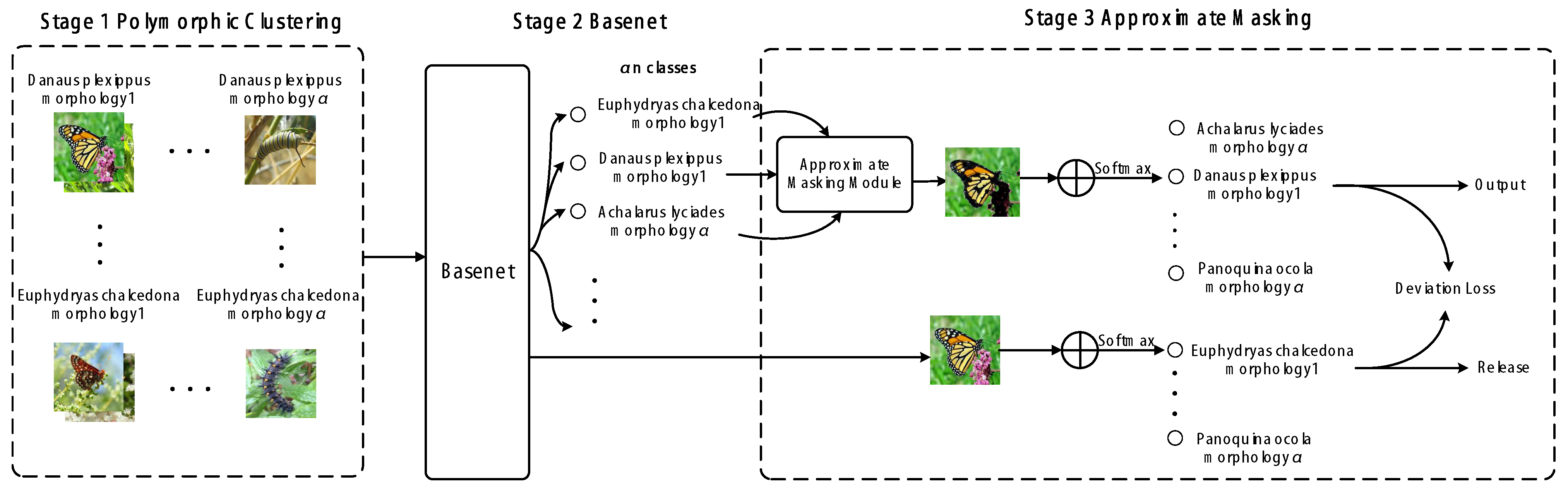
Our proposed PCAM-Frame is primarily divided into three stages. Stage 1 is a novel image data processing method that combines segmentation and clustering operations, which we call the Polymorphic Clustering Module (PCM), which preprocesses insect images before extracting specific features. This preprocessing primarily addresses the significant visual differences in insect individuals at different life stages encountered in fine-grained image classification tasks in insect scenarios. Initially, a transferred salient object segmentation model is used to extract the regions of target insects in the images. This step aims to remove the influence of the background on the next clustering operation. Then, each segmented insect image is subjected to clustering to enable the network to differentiate between individuals of different life stages when learning features. Stage 2 involves feature extraction using a backbone network that has performed well in fine-grained image classification tasks in other scenarios. Stage 3 is a novel masking method, which compares the focus area of the image and filters the area to be occluded with fixed restrictions, called the Approximate Masking Module (AMM), which performs Approximate Masking and Deviation Loss processing for difficult-to-distinguish insect categories after primary feature extraction. This process strengthens the model’s attention to subtle differences between approximate categories during training. The overall framework is illustrated in Figure 2. Since our PCAM-Frame relies on a backbone network, which can be any classification network based on CNN or Transformer, we use "Basenet” to represent the embedding position of the backbone network. Therefore, we will provide detailed explanations of the main content of PCAM-Frame Stage 1 and Stage 3 in detail in the following sections.
3.1. Stage 1: Polymorphic Clustering
This section will elaborate on Stage 1 before feature extraction, which consists of two sub-modules: primary target segmentation and polymorphic clustering. Its purpose is to reclassify individuals of the same subclass of insects at different life stages due to the large appearance difference of the same subclass in different life stages in the insect scene. This allows Basenet to pay attention to the difference in life stages within the class during training, and, to a certain extent, the difference between the insect images of the same life stage is less than the difference within the insect images of different life stages, which has less impact on the final classification of the model. The entire process is depicted in Figure 3.
3.1.1. Salient Object Detection
To ensure accurate differentiation of insect individuals at different life stages through clustering, it is essential to remove the influence of background noise on target insect images. Here, we employ the Salient Object Detection (SOD) method, using the highly acclaimed U2Net network to handle this task. The main structure of U2Net adopts a U-shaped network structure, which includes an encoder (downsampling path) and a decoder (upsampling path). This structure can effectively capture both local and global features in images. It introduces a multiscale feature fusion mechanism in its design, enabling the fusion of feature information from different levels for a more comprehensive understanding of the image. This is particularly helpful for handling targets with large-scale differences. Additionally, it incorporates local perception modules and global perception modules in the network to capture local and global semantic information, aiding in dealing with complex relationships between targets and backgrounds in images. Furthermore, U2Net utilizes attention mechanisms to allow the network to focus more on important areas of the image, thus improving segmentation accuracy. It can predict at high resolution, preserving image details, making it particularly suitable for handling small targets or complex textures. Through this structure, U2Net accurately segments insect targets from complex backgrounds and has begun to be used in recognition and classification tasks [39]. Although there are still some imperfect segmentation cases, it usually removes most of the background noise. Therefore, we use the salient object segmentation method as the first step in preprocessing insect images before extracting specific features.
As shown in Figure 3, insect images have removed the vast majority of background noise after passing through the segmentation network. However, there may still be cases of segmentation errors, such as missing limbs, wings, antennae, etc. Considering that the segmented images are only used as references for subsequent clustering and not as the final input to the feature extraction network, the influence of incorrect segmentation on the final classification can be ignored here.
Here, U2Net accurately segments insect images from the background by designing effective network structures and introducing various feature fusion mechanisms. In our fine-grained insect image classification task in this paper, we utilize this network to perform the first step of processing on each batch of insect images where n is the index of different images in each batch, obtaining segmented images . After overall processing, the image set is obtained.
3.1.2. Polymorphic Clustering
Since the image set ds processed by U2Net has no interference from background noise, the insect subject is revealed, which makes the image more convenient for class clustering. In the images processed by U2Net, there are usually only incomplete or complete insect subjects left in the images. At this time, we use a clustering operation to distinguish them, but the original image is still saved in the end. We perform clustering operations on each segment subset in the segmented image set as follows:
Here, represents the set of data points assigned to the p-th cluster center, represents the Euclidean distance between point x and cluster center c, c represents a certain cluster center of the cluster, in this paper, c represents the category to which the image sample belongs, the first hyperparameter is introduced here, representing the number of categories to be clustered, and then the cluster center is updated:
Finally, the image is segmented after clustering as an index to classify the original image:
Here, n represents the n subclass image set. We adopt the clustering algorithm to cluster each sub-image set after segmentation first to obtain . Here, we do not use the segmentation set after clustering as the input for subsequent feature extraction. Instead, is used as the index of the original dataset before the segmentation, and the image of the dataset before the segmentation is classified into . At this time, the total category number of the dataset is expanded to times of the original dataset.
3.2. Approximate Masking Module
This section elaborates on Stage 3, the AAM, which consists of two sub-methods: the Approximate Masking (AM) method and the Deviation Loss (DL) function. Its purpose is to accurately distinguish the most similar categories, The AM method is a novel masking method, which maps the image to the most likely multiple classes. After comparing the attention regions of these classes, the common attention region is taken as the mask part. This process enhances attention to edge detail differences among these approximate classes to some extent. The structural details are illustrated in Figure 4.
3.2.1. Approximate Masking
As shown in Figure 4, after extracting the final features fn of insect images before classification using the backbone network basenet in the second stage, we first need to identify several classes most likely to be determined as the final category. Here, we introduce a second hyperparameter, , which represents how many easily confused classes are selected for masking. The process of selecting the confusing classes is as follows:
Here, is the final feature of the basenet output, represents the set of all most probable classification categories, and represents the class of the i-th highest probability. Linear regression is applied to map the pre-classification results, and the mapped value represents the classification probability.
Then, we map the obtained set of confusing categories back to the weights in the linear regression function to obtain the feature weight vectors for the most likely classification classes. Subsequently, the regions of interest for these classes are masked. This is achieved by forming a matrix with these vectors and then replacing all elements in each column of the matrix greater than 0 with 0. During masking, we introduce a third hyperparameter to indicate the degree of attention to which regions should be masked. The overall process is as follows:
Here, is the weight mapped back to linear by , is the feature weight vector of class , and is the original weight matrix of class . If all are greater than 0, it means that all the regional features of these classes have a positive effect on the final classification. In this case, if is greater than , it means that the region represented by the change vector is masked; otherwise, it is not processed, and is the new weight matrix after mask processing. Finally, the new weight matrix is obtained, and the new weight matrix is multiplied with the final feature matrix, thus:
Here, in order to facilitate the operation, the rotation rank of the mask matrix is taken and multiplied by the original weight matrix to obtain the new weight matrix . Finally, the obtained by linear regression of the original feature matrix is the classification confidence of the output after the final correction of the network.
3.2.2. Deviation Loss
A batch size contains both different insect samples belonging to the same category and different insect samples belonging to different categories, and these insect samples may be mistakenly classified into similar classes after classification. For the classification results after adding the Approximate Masking Module under ideal conditions, compared with the original classification result without adding a similar region mask module, the recognition accuracy is higher. Here, we propose a novel fusion loss function, called Deviation Loss (DL), which consists of three loss functions with different powers. First of all, we introduce Rankloss [40] to compare the two tensors and , but Rankloss will only produce loss when the classification result is worse than . When similar area mask modules fall into inferior classification accuracy, it is helpful for the Approximate Masking Module to move forward in the direction of better feature effect. Here is:
where y is an indicator vector with an element value of 1 or : a position of 1 indicates that is expected to perform better than , and a position of indicates the opposite. In this paper, in the y vector, except the position of the final classification label corresponding to the sample, which is 1, the other position values are . Obviously, Rankloss only produces loss-directed backpropagation when performs worse than . Therefore, the addition of Rankloss can make the network develop in the direction of positive revenue.
In the first stage, we expanded the total number of categories in the dataset to times the original number by means of clustering, and the classification errors of different forms of the same class were mostly caused by the imbalance of category samples in different life stages of the subclasses after clustering, which was difficult to be solved by the traditional cross-entropy loss function. At this time, we introduce the Focalloss [38] loss function to focus on the problem of classification difficulty imbalance. Here is:
where is the probability that the model predicts the correct class, and is the regulator that controls the weight of easily classified samples. Relative to the cross-entropy loss function, Focalloss has one more . When the is larger (that is, the model can predict the sample more accurately), the value is smaller, so the loss of easily classified samples is reduced. On the contrary, when is small, that is, when the model’s prediction of the sample is inaccurate, the larger the value of , then the loss of easily classified samples will be amplified. This mechanism enables Focal Loss to better deal with category imbalance, which can help the model to better learn the key features of insufficient life stage category samples and improve the classification accuracy.
Therefore, we finally combine these loss functions and finally adopt the DL function that can be expressed as:
where is the sum of the above , , and cross-entropy loss . Through this loss function, the training process of the network can be optimized simply and directly, and the approximate class problem and the imbalance of life stage form samples in insect image classification can be alleviated so that the model is more inclined to the correct classification direction without introducing unnecessary complexity. In summary, the significant target segmentation operation aims to capture small and complex target insect regions in insect images and greatly reduces the interference of background noise on the multi-life stage morphological clustering operation of insects. After clustering each species of insects according to their life stage morphology, the new sample set with category multiplication obtained has a more significant feature extraction effect in the classification network. Then, by masking the confusion area of the approximate class, the attention of its subtle features is further enhanced. Finally, the model is further converged by combining Rankloss, Focalloss and basic cross-entropy loss.
4. Experiments
In this section, we will introduce the detailed setup of experiments and comprehensively evaluate our PCAM-Frame on two fine-grained insect image classification public datasets and two other fine-grained image classification public datasets using multiple mainstream models with the highest accuracy in other fine-grained image classification datasets such as Basenet. Ablation analysis and visualization results are presented to demonstrate the interpretability of PCAM-Frame and the effectiveness of fine-grained image classification in insect scenes.
4.1. Experimental Settings
4.1.1. Datasets
We conducted experiments on four fine-grained image classification public datasets; they are Insecta insect long-tailed distribution in iNaturalist 2017, a large dataset for fine-grained classification of natural biological images distribution subclass dataset, IP102 dataset, the well-known CUB200-2011 bird image fine-grained classification dataset in the field of fine-grained image classification, and the Stanford Cars dataset. Insecta, CUB200-2011, and Stanford Cars dataset’s training and test image distribution were divided according to official guidance documents, while the IP102 dataset had no official guidance documents, so the training set and test set were randomly divided according to 8:2. The reason why we chose CUB200-2011 and Stanford Cars, two non-insect fine-grained image datasets, is to use other fine-grained image classification datasets to confirm the high applicability of our PCAM-Frame in the special case of insect scenes with huge differences in intra-class features. The statistics of training test samples corresponding to each category of the four datasets are shown in Table 1. We used only the images and image labels provided by these datasets in all our experiments, without using any additional annotations.
4.1.2. Detailed Experimental Settings and Evaluation Indicators
In the experiments on Insecta, IP102, CUB200-2011, and Stanford Cars datasets, we first randomly cropped the original image with the size of 224 × 224 and used a random horizontal flip to enhance the data during the image preprocessing in the training stage. In the test phase, we adjusted the image to 256 × 256 size, and then the image was center cropped to 224 × 224 size. In order to ensure the fairness of the experiment, we used the above image preprocessing methods when testing other mainstream models on the two datasets. In the training process of the two datasets, we used the stochastic gradient descent (SGD) optimizer to optimize the model, whose momentum was , the initial learning rate was , and batch size was 16 by default. The cosine annealing function was used to constantly update the learning rate during the training process. The default value of hyperparameter in the first stage experiment of PCAM-Frame was 2, the default value of the number of approximate classes in the mask operation of similar class confusion area in the third stage was 3, and the mask degree was 150.
For all the mainstream fine-grained image classification models used as Basenet in the experiment, we use its pre-trained model parameters without classification headers on ImageNet21k or ImageNet22k as the initial training parameters. Therefore, the comparison between the Transformer class as the backbone network model and the CNN-based model in our experiment is fair and credible. For all comparison experiments related to PCAM-Frame on the four datasets, we adopted precision as the evaluation index, which was defined as follows:
where is the number of correctly predicted samples, and is the total number of predicted samples. All experiments to verify the effectiveness of our approach were performed on the Pytorch platform using a single Nvidia RTX3060 GPU. Here, we use top-1 accuracy as the evaluation criterion.
4.2. Effects of PCAM-Frame on Basenet and Comparison with the Most Advanced Methods
This section describes the effect of PCAM-Frame on the most advanced (SOTA) method for performing fine-grained classification tasks as Basenet on Insecta, IP102, CUB200-2011, and Stanford Cars. At the same time, other CNN-based methods that are not used as Basenet, Vision Transformer-based methods, CNN methods, and Vision Transformer hybrid methods are compared and tested, and the results are obtained and the analysis is completed. In order to ensure the fairness of the comparison experiments, all experiments on our method used the same training hyperparameter settings and test settings. The experimental results are shown in Table 2, in which the experimental accuracy of our method is obtained through the pre-training model provided by the author and other accuracy results are obtained through the relevant literature. Optimal and competitive accuracy are highlighted in bold and underlined, respectively.
4.2.1. Impact Analysis of PCAM-Frame on Basenet in Insecta and IP102 Insect Datasets
From Table 2, we can see that the performance of fine-grained image classification models introduced in the past three years in the insect scenario is not very satisfactory. One reason may be the uneven distribution of sample data in these two insect datasets, but more importantly, it is due to the unique morphology of insects. A significant portion of insect samples contain images from different life stages, and the differences between them are too significant. The uneven distribution of samples from different life stages makes it difficult for these networks to distinguish the specific categories to which these low-sample life-stage insects belong.
However, when the five mainstream networks, VGG-19, ResNet50, ViT-Base, Swin-Base, and Swin-Large, are added to our PCAM-Frame as Basenets, there is a significant improvement in performance on the Insecta and IP102 datasets. The average improvement in accuracy on the Insecta and IP102 datasets reaches 2.2% and 1.4%, respectively, both achieving state-of-the-art (SOTA) results. The difference in accuracy improvement between these two datasets is mainly due to the fact that the IP102 dataset has far fewer samples than Insecta, and the samples of insects in low-sample life stages are even scarcer or missing, resulting in less improvement compared to the large-sample Insecta dataset. This indicates that our PCAM-Frame is more suitable for long-tail datasets with a large number of samples.
4.2.2. Impact Analysis of PCAM-Frame on Basenet in Other Fine-Grained Classification Tasks: CUB200-2011 and Stanford Cars Datasets
As fine-grained image classification tasks have gradually entered the researchers’ field of vision thanks to the development of deep learning neural networks in recent years, there have not been many studies focusing further on fine-grained classification in specific scenarios. The related well-known datasets are also mostly representative. The CUB200-2011 dataset does not have significant differences in appearance between subclasses similar to insects, and the Stanford Cars dataset, as a car dataset, does not have distinctions in appearance based on life stages. Therefore, the life stage clustering in the first stage of the PCAM-Frame may not have a positive effect on the performance of these Basenets on the Stanford Cars dataset.
From Table 2, we can see that the effect of PCAM-Frame on the bird image dataset CUB200-2011 and the car image dataset Stanford Cars is quite limited. The average improvement in accuracy is only 0.4% and 0.1%, respectively, and it even does not exceed the normal accuracy fluctuation range in the experiments. This indicates that our PCAM-Frame is not suitable for image datasets where subclass samples have only one life stage morphology or where the differences in life stage morphology between subclasses are much smaller than the differences between classes.
4.3. Module Ablation Analysis
This section will introduce the accuracy impact of adding different modules of PCAM-Frame to Basenet on the insect image fine-grained classification datasets Insecta and IP102, as well as other fine-grained classification datasets CUB200-2011 and Stanford Cars. To ensure fair comparison experiments, all methods use Swin-Transformer-Base as Basenet, with default hyperparameter values. The same training hyperparameter settings and testing configurations were used for all experiments. The qualitative analysis is shown in Table 3.
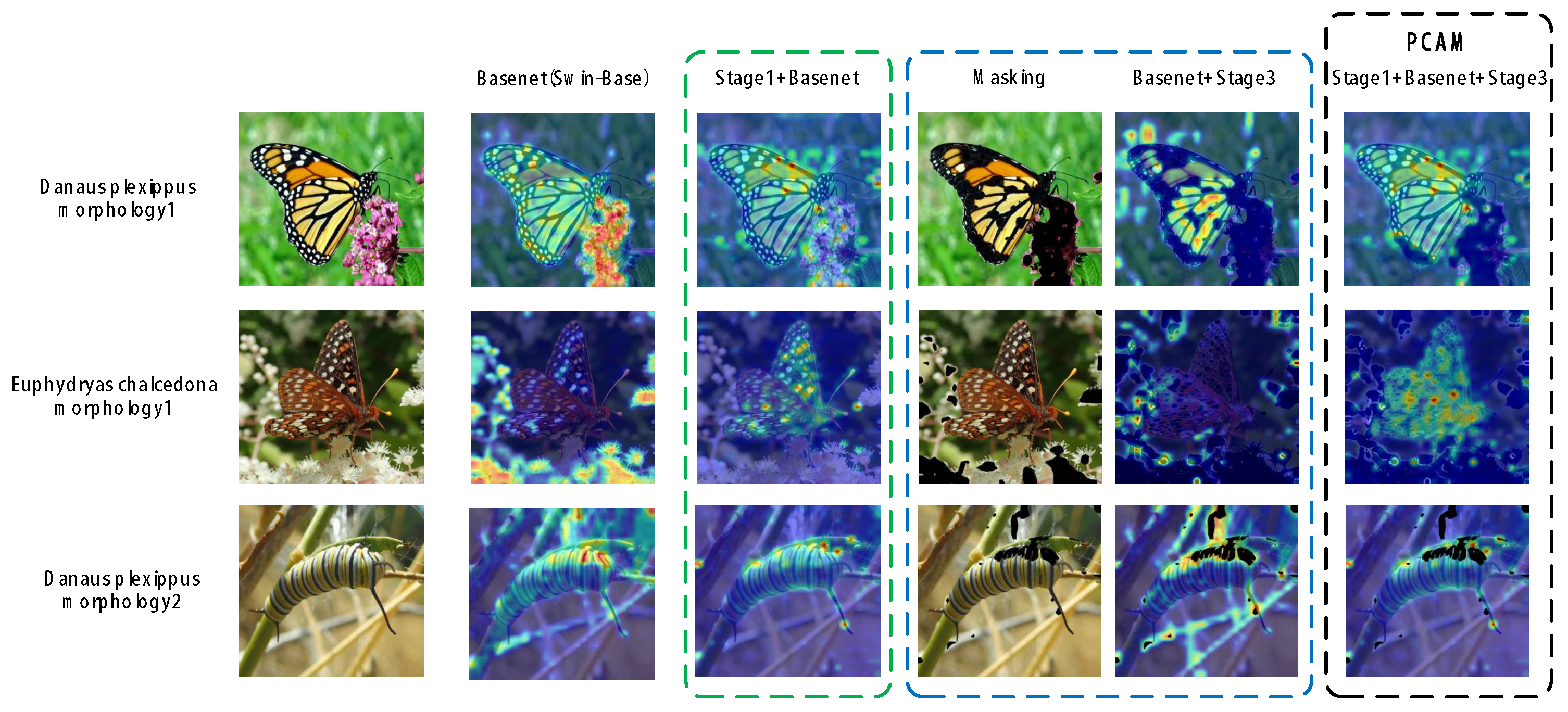
According to Table 3, we can see that our PCAM-Frame, using Swin-Transformer-Base as Basenet, has improved accuracy on all four datasets, with notably better performance in insect scenes. We visualized the regions of interest in insect images from the Insecta dataset using heatmaps for different modules of PCAM-Frame, as shown in Figure 5.
From the heatmaps of the regions of interest for each module in Figure 5, we can intuitively observe that after adding the clustering operation in the first stage, the model focuses more on the main area of the insect target. When the Approximate Masking module in the third stage masks the main conflicting areas of the image, the model pays more attention to the detail area between the approximate classes. The figure visually explains the role of PCAM-Frame at each stage of the fine-grained classification task. This confirms that our research is of great help for insect image fine-grained classification tasks.
We are concerned that the computing speed of the model on the computer changes after the model is applied to the modules of each stage of PCAM-Frame. Therefore, we conduct an experimental discussion on the overall model parameter number and computational complexity after the addition of each module of PCAM-Frame. Resnet50, two Transformer models (ViT-Base, SWI-base) for statistical experiments, and their results are shown in Figure 6.
According to the statistical results of parameters before and after applying PCAM-Frame to the model in the left figure of Figure 6, we can see that the parameters of CNN and Transformer networks have little change after applying PCAM-Frame. This is because U2Net-Lite is embedded in the PCM operation of Stage 1 of PCAM-Frame, and its parameter count is only 4.7 M at the default 224 × 224 size. The mask operation in Stage 3 of PCAM-Frame needs to remap the features into the model. In the CNN class model, the final features of the CNN class model are multiplied with the gradient to map to an attention map. The mapping between cls token and position embedding can obtain the attention map, and the number of model parameters will not increase. The original network classification head is only retrained in the second classification stage, and the number of model parameters will increase very little at this stage. And the Deviation Loss function at the end of PCAM-Frame does not add additional parameters. Therefore, the final number of parameters of each model does not change much after applying PCAM-Frame.
The right figure of Figure 6 is the statistics of Floating Point Operations before and after applying PCAM-Frame to the model. It can be seen that the FLOPs of Transformer network increase greatly, which is because the mask operation of Stage 3 is mapped to patch mapping in the mapping process. Pixel reconstruction in each patch is required, which greatly increases the amount of model computation. However, in CNN-like networks, simple gradient multiplication can be used for mapping, which requires a relatively small amount of computation. Therefore, after applying PCAM-Frame, the training efficiency of CNN-like models is less affected, and the training efficiency of Transformer-like models is significantly reduced.
4.3.1. The Accuracy Effect Analysis of Introducing the Polymorphic Clustering Module in Stage 1
From the experimental results in the fourth row of Table 3, we can see that the model’s accuracy on the insect tasks in the Insecta and IP102 datasets has been improved by 1.9% and 1.0%, respectively, showing significant improvement. However, the accuracy on the bird dataset CUB200-2011 and the car dataset Stanford Cars decreased by 1.2% and 1.5%, respectively. This is because the bird images in the CUB200-2011 dataset are mostly adult birds, and the few juvenile bird samples have very small visual differences from the adult bird samples, making clustering operations unable to distinguish them. Similarly, each type of car in the Stanford Cars dataset does not have different life stage differences, and the clustering operation often groups some car images with different paint colors into one class, ignoring the structural features of the cars, resulting in a decrease in classification accuracy.
Therefore, the Polymorphic Clustering module in the first stage is mainly suitable for fine-grained image classification tasks in scenes with multi-life-stage morphological organisms, such as insects, and is not suitable for image datasets of single-life-stage morphological organisms or artificial objects.
4.3.2. The Accuracy Effect Analysis of Introducing the Approximate Masking Method in Stage 3
From the fifth row of Table 3, it can be seen that directly inputting unprocessed images into the feature extraction network based on Swin-Transformer-Base improves the classification accuracy on all four datasets, with a relatively even improvement effect. This indicates that the Approximate Masking module in the second stage of our PCAM-Frame can be applied to fine-grained image classification tasks in any scene, as it mainly masks the confusing areas of approximate classes, leaving out the distinctive detail areas for the model to make determinations between similar classes.
From the seventh row of Table 3, it can be seen that after clustering the images and inputting them into the feature extraction network based on Swin-Transformer-Base, the model’s accuracy improvement is more significant on insect datasets, while the performance in other scenes is poor. Combined with the results of the fourth row, it can be tentatively concluded that this is due to the influence of the first stage of PCAM-Frame.
4.3.3. The Accuracy Effect Analysis of Introducing Deviation Loss
From the sixth row of Table 3, it can be observed that changing the model’s loss has almost no effect on the model’s accuracy, and the model’s performance even slightly decreases. This is because the new loss is the sum of , , and cross-entropy loss (). At this point, the model does not have a second , so the is 0, and the imbalance of the samples in the four datasets is minimal, causing to hardly update. The average of is close to , resulting in experimental results on the four datasets fluctuating within the normal error range.
From the last three rows of Table 3, it can be inferred that the AM method only has an effect when either the Polymorphic Clustering module in Stage 1 or the AM method in Stage 2 exists, or both modules are present. This is because depends on the AM method, and is heavily influenced by the Polymorphic Clustering module. However, due to the negative impact of the Polymorphic Clustering module on the CUB200-2011 and Stanford Cars datasets, its effectiveness in conjunction with the AM method and DL function can achieve the best results on other scene datasets. Therefore, we consider optimizing the AM method and DL function in subsequent work to achieve better results in fine-grained image classification tasks in other scenes.
In summary, our DL function is a plug-and-play loss function that adds icing on the cake to the performance of our PCAM-Frame in fine-grained image classification tasks in insect scenes.
4.4. Hyperparameters Ablation Study
The discussion in the previous section about the performance of each module is not sufficient to fully explain the motivation behind the selection of the parameters and their default values when designing the PCAM-Frame. Since in Stage 1 and and in Stage 3 do not influence each other, we will conduct separate experiments in this section to discuss the values of the parameter in the Polymorphic Clustering module in Stage 1 and the and parameters in the Approximate Masking module in Stage 3. This will help illustrate the reasons for choosing these parameters and the practical significance of their default values.
4.4.1. Analysis of Hyperparameter in the Polymorphic Clustering Module of Stage 1
Before feeding the image samples from the dataset into the feature extraction network Basenet, we first use the U2Net segmentation network to perform insect object segmentation on the insect images using the segmented insect images as clustering indices. After obtaining the clustering results, the original images are reclassified. This operation aims to distinguish between different life stages of insects, and the number of morphologies specifically needs the hyperparameter to represent. The selection of the specific default value needs to be validated by experiments. Since the Polymorphic Clustering operation in Stage 1 is only effective for insect scene datasets, we only conduct ablation experiments on the parameter on insect datasets. Here, the hyperparameter in the Approximate Masking module is set to the default value of 3, and the hyperparameter is set to the default value of 150 in the experiments. The experimental results are shown in Table 4.
Continuing from Table 4, the average improvement in model classification performance also reached the highest average value when . This may be because most of the samples in the insect classes in the two insect datasets are divided into two life stages. For example, Danaus plexippus, whose images in the Insecta dataset consist of two life stages: larvae and adults. Therefore, when , clustering them into two categories achieved the highest accuracy improvement. At , there is also an improvement in accuracy, possibly because some categories have samples with three or more different life stage morphologies. When is greater than 3, the accuracy decreases. This is because there are too many clustering centers, exceeding the number of life stage morphology categories in the insect sample set, resulting in misalignment during final classification.
4.4.2. Analysis of Hyperparameters and in the Approximate Masking Method of Stage 3
Since the Polymorphic Clustering module in Stage 1 will have a negative impact on fine-grained image classification in non-insect scenes, we will not include the relevant modules from Stage 1 in the ablation experiments in this section. The hyperparameter represents the number of approximate classes the model masks in the Approximate Masking Module, and the hyperparameter represents the degree to which the model focuses on the same region between approximate classes simultaneously in the Approximate Masking Module. Since we use heatmaps to represent the model’s attention to regions in practical coding work, the value of our hyperparameter is between 0 and 255. The influence of hyperparameters and on the model’s accuracy on the Insecta, IP102, CUB200-2011, and Stanford Cars datasets is shown in Figure 7. The Basenet of all experiments is Swin-Base, and the experiments on Insecta and IP102 datasets include Polymorphic Clustering operation in Stage 1. However, CUB200-2011 and Stanford Cars datasets have negative returns on Stage 1 of the experiment, so only Stage 3 operations are conducted for them.
From the 3D confusion matrix plot in Figure 7, we can clearly observe that as increases from 1 to 3, the degree of accuracy improvement of PCAM-Frame on the four datasets gradually rises, reaching its peak at . Beyond , there is no significant change in accuracy, and further increases in would lead to a substantial increase in computational complexity for the Polymorphic Clustering module, which is not conducive to the model’s subsequent improvement. On the other hand, the value of has a greater impact on model performance. When is less than 110, the model’s performance is lower than the original network, as is too small, resulting in too many masked regions where the model cannot capture useful classification information from the remaining image areas. When , the model’s accuracy exceeds that of Basenet, and at , the model’s accuracy reaches its peak. However, when exceeds 150, the masked regions become too few, causing negative effects on the model’s discrimination between approximate classes, resulting in a gradual decline in performance, even lower than that of Basenet. In summary, with and , the Approximate Masking Module achieves the highest accuracy improvement. Therefore, the default values of and used in our comparative experiments are set to 3 and 150, respectively.
5. Discussion
Fine-grained image classification in insect scenes is a problem with higher complexity. As we can see visually, individual insects often evolve color textures that are highly similar to the surrounding vegetation according to the ecological environment they live in, making them more difficult to capture compared to other individual animals. This is the first acute challenge. What is more, unlike other animals, insects do not just change in size or proportion of body parts during the transition of each life stage. There are often no visual similarities between different life stages, which is the most difficult challenge in insect classification.
These two challenges cannot be solved by a single network model and require additional human processing. However, spending a lot of manpower and money on anchoring and life stages is contrary to the purpose of our deep learning technology. We need an automated framework to transfer existing techniques from other domains or come up with new improvements to solve challenges in insect scenario.
As the above experimental results show, our PCAM-Frame has achieved good performance in the insect scene, which is the effectiveness of our proposed targeted solutions to the above two acute problems. Specifically, the PCM in Stage 1 of our PCAM-Frame plays a positive role, which roughly segments the insect individuals in the insect image samples and isolates the influence of the environmental background noise on the clustering operation. The combination of the two operations allows us to automatically distinguish the insect images according to the life stage form. The insect images are labeled with the life stage labels to avoid confusing the class features of insects with different life stage samples without visual association. For AMM in Stage 2, according to the experimental results, it shows a certain degree of universality, and it is still possible to be transferred to fine-grained image classification tasks in other scenes. This is because the AM method is not proposed for the unique difficulties of insects. This problem of final classification of approximate classes is likely to be encountered in many fine-grained image classification scenarios, which is also confirmed by the ablation experiments in Table 3.
In the process of practical application, there are still some potential challenges that our PCAM-Frame will face soon. In the process of actual use, new insect samples will be registered in real time, and registered unqualified insect samples will also be removed in real time. After new samples are registered, new class features are brought, but also a sample imbalance problem is generated, although PCAM-Frame can rely on the DL function of Stage 3 to alleviate this problem dynamically. However, before the unqualified insect sample is removed, it has already brought pollution to the model, and these misguidance parameters cannot be accurately removed from the model, and the model is not easy to retrain in the process of removing the wrong sample, which is the limitation of our PCAM-Frame framework. Therefore, we subsequently consider adding a sample screening module to Stage 2 of PCAM-Frame to dynamically eliminate those unqualified samples according to the sample evaluation after the samples are input into the network, so as to keep the model from being contaminated during the training process.
6. Conclusions
This paper proposes a training framework called PCAM-Frame for insect image fine-grained classification tasks, addressing the challenges caused by the significant morphological differences across multiple life stages within insect categories and the large amount of confusion between similar insect categories, and to meet the adaptation of mainstream fine-grained image classification networks to insect scenes. Built upon the backbone network (Basenet), the PCAM-Frame framework conducts primary target segmentation and polymorphic clustering before inputting into the network, allowing Basenet to learn intra-class life stage morphological characteristics. After extracting network output features, the framework employs approximate masking of confusing regions between similar classes to mask out invalid features and enhance the weight of detailed features. Finally, multiple loss functions are combined to ensure the model converges optimally. The PCAM-Frame structure is well organized, easy to deploy, and can be flexibly adjusted according to the characteristics of Basenet and the classification task. Excellent results have been achieved on the Insecta and IP102 insect image datasets. We demonstrate that our PCAM-Frame brings a good adaptation to mainstream fine-grained image classification networks in insect scenarios. We conducted thorough ablation experiments on the framework’s stages and hyperparameters, fully validating and discussing the actual effects of each stage of the PCAM-Frame and the rationale behind the default parameter settings.
In the future, we plan to incorporate some data augmentation operations during polymorphic clustering to maintain a more balanced distribution of samples for each morphological form of individual insect classes. Additionally, based on the best performance of several Basenet structures, we try to design a feature extraction network specially suitable for our PCAM-Frame to achieve better results in fine-grained insect image classification tasks. Furthermore, we will optimize the design of loss functions to find new function structures that not only ensure the model converges optimally but also accelerate convergence speed.
Author Contributions
Conceptualization, A.M. and H.H.; methodology, A.M.; software, A.M.; validation, A.M., H.H. and N.X.; formal analysis, A.M.; investigation, A.M.; resources, H.H.; data curation, N.X.; writing—original draft preparation, A.M.; writing—review and editing, A.M.; visualization, N.X.; supervision, A.M.; project administration, A.M.; funding acquisition, H.H. All authors have read and agreed to the published version of the manuscript.
Funding
This work was partially supported by the National Natural Science Foundation of China (61672210), the Major Science and Technology Program of Henan Province (221100210500), and the Central Government Guiding Local Science and Technology Development Fund Program of Henan Province (Z20221343032).
Data Availability Statement
The data presented in this study are available on request from the corresponding author.
Conflicts of Interest
The authors declare no conflicts of interest.
References
- Wah, C.; Branson, S.; Welinder, P.; Perona, P.; Belongie, S. The Caltech-UCSD Birds-200-2011 Dataset. California Institute of Technology, 2011. Available online: https://authors.library.caltech.edu/records/cvm3y-5hh21 (accessed on 23 May 2023).
- Khosla, A.; Jayadevaprakash, N.; Yao, B.; Li, F.-F. Novel Dataset for Fine-Grained Image Categorization. 2013. Available online: https://people.csail.mit.edu/khosla/papers/fgvc2011.pdf (accessed on 23 May 2023).
- Van Horn, G.; Mac Aodha, O.; Song, Y.; Cui, Y.; Sun, C.; Shepard, A.; Adam, H.; Perona, P.; Belongie, S. The inaturalist species classification and detection dataset. In Proceedings of the IEEE Conference on Computer Vision and Pattern Recognition, Salt Lake City, UT, USA, 18–23 June 2018; pp. 8769–8778. [Google Scholar]
- Wu, X.; Zhan, C.; Lai, Y.K.; Cheng, M.M.; Yang, J. Ip102: A large-scale benchmark dataset for insect pest recognition. In Proceedings of the IEEE/CVF Conference on Computer Vision and Pattern Recognition, Long Beach, CA, USA, 15–20 June 2019; pp. 8787–8796. [Google Scholar]
- Krause, J.; Stark, M.; Deng, J.; Fei-Fei, L. 3D Object Representations for Fine-Grained Categorization. In Proceedings of the IEEE International Conference on Computer Vision Workshops, Columbus, OH, USA, 23–28 June 2014. [Google Scholar]
- Maji, S.; Rahtu, E.; Kannala, J.; Blaschko, M.; Vedaldi, A. Fine-grained visual classification of aircraft. arXiv, 2013; arXiv:1306.5151. [Google Scholar]
- LeCun, Y.; Bottou, L.; Bengio, Y.; Haffner, P. Gradient-based learning applied to document recognition. Proc. IEEE 1998, 86, 2278–2324. [Google Scholar] [CrossRef]
- Vaswani, A.; Shazeer, N.; Parmar, N.; Uszkoreit, J.; Jones, L.; Gomez, A.N.; Kaiser, Ł.; Polosukhin, I. Attention is all you need. Adv. Neural Inf. Process. Syst. 2017, 30. [Google Scholar]
- Dosovitskiy, A.; Beyer, L.; Kolesnikov, A.; Weissenborn, D.; Zhai, X.; Unterthiner, T.; Dehghani, M.; Minderer, M.; Heigold, G.; Gelly, S.; et al. An image is worth 16x16 words: Transformers for image recognition at scale. arXiv 2020, arXiv:2010.11929. [Google Scholar]
- Lowe, D.G. Distinctive image features from scale-invariant keypoints. Int. J. Comput. Vis. 2004, 60, 91–110. [Google Scholar] [CrossRef]
- Dalal, N.; Triggs, B. Histograms of oriented gradients for human detection. In Proceedings of the 2005 IEEE Computer Society Conference on Computer Vision and Pattern Recognition (CVPR’05), San Diego, CA, USA, 20–25 June 2005; Volume 1, pp. 886–893. [Google Scholar]
- Lin, T.Y.; RoyChowdhury, A.; Maji, S. Bilinear CNN models for fine-grained visual recognition. In Proceedings of the IEEE International Conference on Computer Vision, Santiago, Chile, 7–13 December 2015; pp. 1449–1457. [Google Scholar]
- Zhuang, P.; Wang, Y.; Qiao, Y. Learning attentive pairwise interaction for fine-grained classification. In Proceedings of the AAAI Conference on Artificial Intelligence, New York, NY, USA, 7–12 February 2020; Volume 34, pp. 13130–13137. [Google Scholar]
- Sun, Y.; Zheng, L.; Yang, Y.; Tian, Q.; Wang, S. Beyond part models: Person retrieval with refined part pooling (and a strong convolutional baseline). In Proceedings of the European Conference on Computer Vision (ECCV), Munich, Germany, 8–14 September 2018; pp. 480–496. [Google Scholar]
- Xie, S.; Girshick, R.; Dollár, P.; Tu, Z.; He, K. Aggregated residual transformations for deep neural networks. In Proceedings of the IEEE Conference on Computer Vision and Pattern Recognition, Honolulu, HI, USA, 21–26 July 2017; pp. 1492–1500. [Google Scholar]
- Liu, H.; Tian, Y.; Yang, Y.; Pang, L.; Huang, T. Deep relative distance learning: Tell the difference between similar vehicles. In Proceedings of the IEEE Conference on Computer Vision and Pattern Recognition, Las Vegas, NV, USA, 27–30 June 2016; pp. 2167–2175. [Google Scholar]
- He, J.; Chen, J.N.; Liu, S.; Kortylewski, A.; Yang, C.; Bai, Y.; Wang, C. Transfg: A transformer architecture for fine-grained recognition. In Proceedings of the AAAI Conference on Artificial Intelligence, Philadelphia, PA, USA, 22 February–1 March 2022; Volume 36, pp. 852–860. [Google Scholar]
- Liu, X.; Wang, L.; Han, X. Transformer with peak suppression and knowledge guidance for fine-grained image recognition. Neurocomputing 2022, 492, 137–149. [Google Scholar] [CrossRef]
- Liu, Z.; Lin, Y.; Cao, Y.; Hu, H.; Wei, Y.; Zhang, Z.; Lin, S.; Guo, B. Swin transformer: Hierarchical vision transformer using shifted windows. In Proceedings of the IEEE/CVF International Conference on Computer Vision, Montreal, BC, Canada, 11–17 October 2021; pp. 10012–10022. [Google Scholar]
- Sun, H.; He, X.; Peng, Y. Sim-trans: Structure information modeling transformer for fine-grained visual categorization. In Proceedings of the 30th ACM International Conference on Multimedia, Lisbon, Portugal, 10–14 October 2022; pp. 5853–5861. [Google Scholar]
- Bera, A.; Wharton, Z.; Liu, Y.; Bessis, N.; Behera, A. Sr-gnn: Spatial relation-aware graph neural network for fine-grained image categorization. IEEE Trans. Image Process. 2022, 31, 6017–6031. [Google Scholar] [CrossRef]
- Chou, P.Y.; Kao, Y.Y.; Lin, C.H. Fine-grained visual classification with high-temperature refinement and background suppression. arXiv 2023, arXiv:2303.06442. [Google Scholar]
- Pucci, R.; Kalkman, V.J.; Stowell, D. Comparison between transformers and convolutional models for fine-grained classification of insects. arXiv 2023, arXiv:2307.11112. [Google Scholar]
- Larios, N.; Deng, H.; Zhang, W.; Sarpola, M.; Yuen, J.; Paasch, R.; Moldenke, A.; Lytle, D.A.; Correa, S.R.; Mortensen, E.N.; et al. Automated insect identification through concatenated histograms of local appearance features: Feature vector generation and region detection for deformable objects. Mach. Vis. Appl. 2008, 19, 105–123. [Google Scholar] [CrossRef]
- Faithpraise, F.; Birch, P.; Young, R.; Obu, J.; Faithpraise, B.; Chatwin, C. Automatic plant pest detection and recognition using k-means clustering algorithm and correspondence filters. Int. J. Adv. Biotechnol. Res. 2013, 4, 189–199. [Google Scholar]
- Zhu, L.Q.; Zhang, Z. Auto-classification of insect images based on color histogram and GLCM. In Proceedings of the 2010 7th International Conference on Fuzzy Systems and Knowledge Discovery, Yantai, China, 10–12 August 2010; Volume 6, pp. 2589–2593. [Google Scholar]
- Cheng, X.; Zhang, Y.; Chen, Y.; Wu, Y.; Yue, Y. Pest identification via deep residual learning in complex background. Comput. Electron. Agric. 2017, 141, 351–356. [Google Scholar] [CrossRef]
- Xie, C.; Li, R.; Dong, W.; Song, L.; Zhang, J.; Chen, H.; Chen, T. Recognition for insects via spatial pyramid model using sparse coding. Trans. Chin. Soc. Agric. Eng. 2016, 32, 144–151. [Google Scholar]
- Korsch, D.; Bodesheim, P.; Denzler, J. Deep learning pipeline for automated visual moth monitoring: Insect localization and species classification. arXiv 2023, arXiv:2307.15427. [Google Scholar]
- Theivaprakasham, H.; Darshana, S.; Ravi, V.; Sowmya, V.; Gopalakrishnan, E.; Soman, K. Odonata identification using customized convolutional neural networks. Expert Syst. Appl. 2022, 206, 117688. [Google Scholar] [CrossRef]
- Peng, Y.; Wang, Y. CNN and transformer framework for insect pest classification. Ecol. Inform. 2022, 72, 101846. [Google Scholar] [CrossRef]
- Le-Qing, Z.; Zhen, Z. Automatic insect classification based on local mean colour feature and Supported Vector Machines. Orient. Insects 2012, 46, 260–269. [Google Scholar] [CrossRef]
- Dembski, J.; Szymański, J. Bees detection on images: Study of different color models for neural networks. In Proceedings of the Distributed Computing and Internet Technology: 15th International Conference, ICDCIT 2019, Bhubaneswar, India, 10–13 January 2019; pp. 295–308. [Google Scholar]
- Chawla, N.V.; Bowyer, K.W.; Hall, L.O.; Kegelmeyer, W.P. SMOTE: Synthetic minority over-sampling technique. J. Artif. Intell. Res. 2002, 16, 321–357. [Google Scholar] [CrossRef]
- He, H.; Bai, Y.; Garcia, E.A.; Li, S. ADASYN: Adaptive synthetic sampling approach for imbalanced learning. In Proceedings of the 2008 IEEE International Joint Conference on Neural Networks (IEEE World Congress on Computational Intelligence), Hong Kong, China, 1–6 June 2008; pp. 1322–1328. [Google Scholar]
- Wu, D.; Xu, Y.; Lu, B.L. Transfer learning for EEG-based brain–computer interfaces: A review of progress made since 2016. IEEE Trans. Cogn. Dev. Syst. 2020, 14, 4–19. [Google Scholar] [CrossRef]
- Tang, S.; Wang, C.; Nie, J.; Kumar, N.; Zhang, Y.; Xiong, Z.; Barnawi, A. EDL-COVID: Ensemble deep learning for COVID-19 case detection from chest X-ray images. IEEE Trans. Ind. Inform. 2021, 17, 6539–6549. [Google Scholar] [CrossRef]
- Lin, T.Y.; Goyal, P.; Girshick, R.; He, K.; Dollár, P. Focal loss for dense object detection. In Proceedings of the IEEE International Conference on Computer Vision, Venice, Italy, 22–29 October 2017; pp. 2980–2988. [Google Scholar]
- Gamage, L.; Isuranga, U.; Meedeniya, D.; De Silva, S.; Yogarajah, P. Melanoma Skin Cancer Identification with Explainability Utilizing Mask Guided Technique. Electronics 2024, 13, 680. [Google Scholar] [CrossRef]
- Briggs, F.; Fern, X.Z.; Raich, R. Rank-loss support instance machines for MIML instance annotation. In Proceedings of the 18th ACM SIGKDD International Conference on Knowledge Discovery and Data Mining, Beijing, China, 12–16 August 2012; pp. 534–542. [Google Scholar]
- Simonyan, K.; Zisserman, A. Very deep convolutional networks for large-scale image recognition. arXiv 2014, arXiv:1409.1556. [Google Scholar]
- Fu, J.; Zheng, H.; Mei, T. Look closer to see better: Recurrent attention convolutional neural network for fine-grained image recognition. In Proceedings of the IEEE Conference on Computer Vision and Pattern Recognition, Honolulu, HI, USA, 21–26 July 2017; pp. 4438–4446. [Google Scholar]
- He, K.; Zhang, X.; Ren, S.; Sun, J. Deep residual learning for image recognition. In Proceedings of the IEEE Conference on Computer Vision and Pattern Recognition, Las Vegas, NV, USA, 27–30 June 2016; pp. 770–778. [Google Scholar]
- Chen, Y.; Bai, Y.; Zhang, W.; Mei, T. Destruction and construction learning for fine-grained image recognition. In Proceedings of the IEEE/CVF Conference on Computer Vision and Pattern Recognition, Long Beach, CA, USA, 15–20 June 2019; pp. 5157–5166. [Google Scholar]
- Szegedy, C.; Ioffe, S.; Vanhoucke, V.; Alemi, A. Inception-v4, inception-resnet and the impact of residual connections on learning. In Proceedings of the AAAI Conference on Artificial Intelligence, San Francisco, CA, USA, 4–9 February 2017; Volume 31. [Google Scholar]
- Liu, C.; Xie, H.; Zha, Z.J.; Ma, L.; Yu, L.; Zhang, Y. Filtration and distillation: Enhancing region attention for fine-grained visual categorization. In Proceedings of the AAAI Conference on Artificial Intelligence, New York, NY, USA, 7–12 February 2020; Volume 34, pp. 11555–11562. [Google Scholar]
- Song, J.; Yang, R. Feature boosting, suppression, and diversification for fine-grained visual classification. In Proceedings of the 2021 International Joint Conference on Neural Networks (IJCNN), Shenzhen, China, 18–22 July 2021; pp. 1–8. [Google Scholar]
- Ge, W.; Lin, X.; Yu, Y. Weakly supervised complementary parts models for fine-grained image classification from the bottom up. In Proceedings of the IEEE/CVF Conference on Computer Vision and Pattern Recognition, Long Beach, CA, USA, 15–20 June 2019; pp. 3034–3043. [Google Scholar]
- Zhang, Y.; Cao, J.; Zhang, L.; Liu, X.; Wang, Z.; Ling, F.; Chen, W. A free lunch from vit: Adaptive attention multi-scale fusion transformer for fine-grained visual recognition. In Proceedings of the ICASSP 2022-2022 IEEE International Conference on Acoustics, Speech and Signal Processing (ICASSP), Singapore, 22–27 May 2022; pp. 3234–3238. [Google Scholar]
- Wang, J.; Yu, X.; Gao, Y. Feature fusion vision transformer for fine-grained visual categorization. arXiv 2021, arXiv:2107.02341. [Google Scholar]
- Xu, Q.; Wang, J.; Jiang, B.; Luo, B. Fine-grained visual classification via internal ensemble learning transformer. IEEE Trans. Multimed. 2023, 25, 9015–9028. [Google Scholar] [CrossRef]
- Chou, P.Y.; Lin, C.H.; Kao, W.C. A novel plug-in module for fine-grained visual classification. arXiv 2022, arXiv:2202.03822. [Google Scholar]
- Zhu, H.; Ke, W.; Li, D.; Liu, J.; Tian, L.; Shan, Y. Dual cross-attention learning for fine-grained visual categorization and object re-identification. In Proceedings of the IEEE/CVF Conference on Computer Vision and Pattern Recognition, New Orleans, LA, USA, 18–24 June 2022; pp. 4692–4702. [Google Scholar]
- Wu, H.; Xiao, B.; Codella, N.; Liu, M.; Dai, X.; Yuan, L.; Zhang, L. Cvt: Introducing convolutions to vision transformers. In Proceedings of the IEEE/CVF International Conference on Computer Vision, Montreal, BC, Canada, 11–17 October 2021; pp. 22–31. [Google Scholar]
- Chen, Y.; Dai, X.; Chen, D.; Liu, M.; Dong, X.; Yuan, L.; Liu, Z. Mobile-former: Bridging mobilenet and transformer. In Proceedings of the IEEE/CVF Conference on Computer Vision and Pattern Recognition, New Orleans, LA, USA, 18–24 June 2022; pp. 5270–5279. [Google Scholar]
Figure 1.
Partial samples from the Insecta subset of the iNaturalist 2017 dataset.

Figure 2.
Overall structure of PCAM-Frame. It consists of three stages from left to right: Stage 1 Polymorphic Clustering is represented in the dashed box on the left, which is mainly completed by segmentation and clustering operations. The middle rounded rectangular box represents Stage 2 Basenet, which represents the embedding position of the backbone network. The dashed box on the right represents Stage 3 Approximate Masking, which consists of two parts: image mask and deviation loss.

Figure 3.
Stage 1: salient object detection and polymorphic clustering. Firstly, U2Net was used to perform Salient Object Detection (SOD) operation, and then the SOD results were used to perform k-means clustering on the original image set.
Figure 3.
Stage 1: salient object detection and polymorphic clustering. Firstly, U2Net was used to perform Salient Object Detection (SOD) operation, and then the SOD results were used to perform k-means clustering on the original image set.

Figure 4.
Stage 3: region masking and deviation loss. Firstly, the pre-classification is performed, and then the image mask is performed according to the mapping of the pre-classification results. Finally, the Deviation Loss is used to correct the convergence direction.
Figure 4.
Stage 3: region masking and deviation loss. Firstly, the pre-classification is performed, and then the image mask is performed according to the mapping of the pre-classification results. Finally, the Deviation Loss is used to correct the convergence direction.

Figure 5.
Visualization of areas of interest for different modules of PCAM-Frame on Insecta dataset.
Figure 5.
Visualization of areas of interest for different modules of PCAM-Frame on Insecta dataset.

Figure 6.
Parameter number and Floating Point Operations (FLOPs) statistics of mainstream Basenet after applying PCAM-Frame.
Figure 6.
Parameter number and Floating Point Operations (FLOPs) statistics of mainstream Basenet after applying PCAM-Frame.

Figure 7.
Hyperparameter analysis of and on all four datasets. Blue represents lower accuracy than Basenet without adding Stage 3, and the closer to blue means the lower accuracy of the model at that parameter value. On the contrary, the red represents higher accuracy than Basenet without adding Stage 3, and the closer to red means the higher accuracy of the model at that parameter value.


Table 1.
Summary of the total number of categories and training–testing sample statistics for the four datasets.
Table 1.
Summary of the total number of categories and training–testing sample statistics for the four datasets.
| Dataset | Class | Total Images | Train Images | Test Images |
|---|---|---|---|---|
| Insecta [3] | 1021 | 118,555 | 100,479 | 18,076 |
| IP102 [4] | 102 | 75,222 | 60,177 | 15,045 |
| CUB-200-2011 [1] | 200 | 11,788 | 5994 | 5794 |
| Stanford Cars [2] | 196 | 16,185 | 8144 | 8041 |
Table 2.
Comparison of top-1 accuracy on Insecta, IP102, CUB200-2011, and Stanford Cars datasets.
| Method | BackBone | Acc(%)/Insecta | Acc(%)/IP102 | Acc(%)/CUB | Acc(%)/Cars |
|---|---|---|---|---|---|
| VGG-19 [41] | VGG-19 | 52.7 | 48.7 | 84.0 | 91.8 |
| RA-CNN [42] | VGG-19 | 53.3 | 48.8 | 85.3 | 92.5 |
| ResNet-50 [43] | ResNet-50 | 54.1 | 49.5 | 84.5 | 92.7 |
| DCL [44] | ResNet-50 | 54.0 | 49.4 | 87.4 | 94.4 |
| ResNet-152 [43] | ResNet-152 | 54.2 | 49.3 | 86.6 | 93.6 |
| SSN [45] | ResNet-101 | 54.9 | 49.9 | 86.7 | - |
| FDL [46] | DenseNet-161 | 55.0 | - | 89.1 | 94.3 |
| FBSD [47] | ResNet-50 | 55.1 | - | 89.3 | 94.4 |
| API-Net [13] | DenseNet-161 | 55.3 | 50.4 | 90.0 | 95.3 |
| StackedLSTM [48] | GoogleNet | 56.0 | 51.0 | 90.4 | - |
| ViT [9] | ViT-Base | 57.7 | 51.9 | 90.2 | 93.6 |
| AFtrans [49] | ViT-Base | 58.2 | 52.2 | 91.5 | 95.0 |
| TransFG [17] | ViT-Base | 58.4 | 52.3 | 91.7 | 94.8 |
| FFVT [50] | ViT-Base | 58.4 | 52.4 | 91.6 | 94.4 |
| IELT [51] | ViT-Base | 58.4 | 52.9 | 91.8 | 94.8 |
| Swin-Trans [19] | Swin-Base | 58.8 | 52.9 | 92.0 | 94.9 |
| SIM-Trans [20] | Swin-Base | 58.9 | 53.0 | 91.8 | - |
| PIM [52] | Swin-Large | 60.9 | 53.3 | 92.4 | 95.1 |
| HERBS [22] | Swin-Base | 60.6 | 54.0 | 93.1 | - |
| DCAL [53] | ResNet-50+ViT-Base | 60.4 | 52.6 | 92.0 | 95.3 |
| CvT [54] | ResNet-50+ViT-Base | 60.0 | 52.3 | 91.2 | - |
| Mobile-Former [55] | MobileNet+ViT-Base | 60.9 | 53.2 | 92.4 | - |
| Our PCAM-Frame | VGG-19 | 55.0 (+2.3) | 49.9 (+1.2) | 83.9 (+0.1) | 92.0 (+0.2) |
| Our PCAM-Frame | ResNet-50 | 55.7 (+1.6) | 50.4 (+0.9) | 84.7 (+0.2) | 93.0 (+0.3) |
| Our PCAM-Frame | ViT-Base | 60.0 (+2.3) | 53.4 (+1.5) | 91.1 (+0.9) | 93.3 (−0.3) |
| Our PCAM-Frame | Swin-Base | 61.6 (+2.8) | 54.7 (+1.8) | 92.4 (+0.4) | 95.0(+0.1) |
| Our PCAM-Frame | Swin-Large | 63.1 (+2.2) | 54.9 (+1.6) | 92.7 (+0.3) | 95.1 (+0) |
The numbers in parentheses indicate that PCAM-Frame improves the performance of the current backbone network.
Table 3.
The top-1 accuracy of each module of PCAM-Frame is compared on Insecta, IP102, CUB200-2011 and Stanford Cars datasets.
Table 3.
The top-1 accuracy of each module of PCAM-Frame is compared on Insecta, IP102, CUB200-2011 and Stanford Cars datasets.
| Module | Acc(%)/Insecta | Acc(%)/IP102 | Acc(%)/CUB | Acc(%)/Cars | ||
|---|---|---|---|---|---|---|
| Stage1-PCM | Stage3-AM | Stage3-DL | ||||
| 58.8 | 52.9 | 92.0 | 94.9 | |||
| ✓ | 60.7 (+1.9) | 53.9 (+1.0) | 90.8 (−1.2) | 93.4 (−1.5) | ||
| ✓ | 59.7 (+0.9) | 53.3 (+0.4) | 92.7 (+0.7) | 95.1 (+0.2) | ||
| ✓ | 58.6 (−0.2) | 52.3 (−0.6) | 92.0 (+0) | 94.4 (−0.5) | ||
| ✓ | ✓ | 61.0 (+2.2) | 54.3 (+1.4) | 92.2 (+0.2) | 94.8 (−0.1) | |
| ✓ | ✓ | 60.9 (+2.1) | 54.1 (+1.2) | 91.6 (−0.4) | 94.1 (−0.8) | |
| ✓ | ✓ | 60.2 (+1.4) | 54.7 (+1.8) | 92.5 (+0.5) | 95.0 (+0.1) | |
| ✓ | ✓ | ✓ | 61.6 (+2.8) | 54.7 (+1.8) | 92.4 (+0.4) | 95.0 (+0.1) |
The numbers in parentheses indicate the impact of each module of PCAM-Frame on the accuracy of Basenet on the insect datasets.
Table 4.
Hyperparameter analysis of on Insecta and IP102.
| Parameter Value () | Module (Basenet:Swin-Base) | Acc(%)/Insecta | Acc(%)/IP102 |
|---|---|---|---|
| 1 | Stage1 + Basenet | 58.8 | 52.9 |
| 1 | Stage1 + Basenet + Stage3 | 58.6 | 52.2 |
| 2 | Stage1 + Basenet | 60.7 (+1.9) | 53.9 (+1.0) |
| 2 | Stage1 + Basenet + Stage3 | 61.6 (+3.0) | 54.7 (+2.5) |
| 3 | Stage1 + Basenet | 60.8 (+2.0) | 53.0 (+0.1) |
| 3 | Stage1 + Basenet + Stage3 | 61.0 (+2.4) | 53.4 (+1.2) |
| 4 | Stage1 + Basenet | 56.4 (−2.4) | 51.8 (−1.1) |
| 4 | Stage1 + Basenet + Stage3 | 56.7 (−1.9) | 51.7 (−0.5) |
| 5 | Stage1 + Basenet | 54.7 (−4.1) | 52.0 (−0.9) |
| 5 | Stage1 + Basenet + Stage3 | 55.1 (−3.5) | 51.7 (−0.5) |
The numbers in parentheses indicate the impact of the individual modules of PCAM-Frame on the accuracy of Basenet on the insect datasets.
Disclaimer/Publisher’s Note: The statements, opinions and data contained in all publications are solely those of the individual author(s) and contributor(s) and not of MDPI and/or the editor(s). MDPI and/or the editor(s) disclaim responsibility for any injury to people or property resulting from any ideas, methods, instructions or products referred to in the content. |
© 2024 by the authors. Licensee MDPI, Basel, Switzerland. This article is an open access article distributed under the terms and conditions of the Creative Commons Attribution (CC BY) license (https://creativecommons.org/licenses/by/4.0/).
Share and Cite
MDPI and ACS Style
Huo, H.; Mei, A.; Xu, N. Polymorphic Clustering and Approximate Masking Framework for Fine-Grained Insect Image Classification. Electronics 2024, 13, 1691. https://doi.org/10.3390/electronics13091691
AMA Style
Huo H, Mei A, Xu N. Polymorphic Clustering and Approximate Masking Framework for Fine-Grained Insect Image Classification. Electronics. 2024; 13(9):1691. https://doi.org/10.3390/electronics13091691
Chicago/Turabian StyleHuo, Hua, Aokun Mei, and Ningya Xu. 2024. "Polymorphic Clustering and Approximate Masking Framework for Fine-Grained Insect Image Classification" Electronics 13, no. 9: 1691. https://doi.org/10.3390/electronics13091691
Note that from the first issue of 2016, this journal uses article numbers instead of page numbers. See further details here.