
An Enhanced Hidden Markov Model for Map-Matching in Pedestrian Navigation

Computer Engineering Department, Kwangwoon University, Seoul 01897, Republic of Korea
*
Author to whom correspondence should be addressed.
†
These authors contributed equally to the article and share first authorship.
Electronics 2024, 13(9), 1685; https://doi.org/10.3390/electronics13091685
Submission received: 20 February 2024
/
Revised: 20 April 2024
/
Accepted: 24 April 2024
/
Published: 26 April 2024
(This article belongs to the Special Issue Recent Research in Positioning and Activity Recognition Systems)
Abstract
:Map-matching is a core functionality of pedestrian navigation applications. The localization errors of the global positioning systems (GPSs) in smartphones are one of the most critical factors that limit the large-scale deployment of pedestrian navigation applications, especially in dense urban areas where multiple road segments exist within the range of GPS errors, which can be increased by tall buildings neighboring each other. In this paper, we address two issues of practical importance for map-matching based on the Hidden Markov Model (HMM) in pedestrian navigation systems: large localization error in the initial phase of map-matching and HMM breaks in open field traversals. A heuristic method to determine the probability of initial states of the HMM based on a small number of GPS data received during the short warm-up period is proposed to improve the accuracy of initial map-matching. A simple but highly practical method based on a heuristic evaluation of near-future locations is proposed to prevent the malfunction of the Viterbi algorithm within the area of open fields. The results of field experiments indicate that the enhanced HMM constructed via the proposed methods achieves significantly higher map-matching accuracy compared to that of state of the art.
1. Introduction
Pedestrian navigation refers to the technology or systems designed to assist individuals in locating, tracking, and following routes to reach a specific destination on foot, primarily using smartphones equipped with a GPS receiver [1]. Map-matching is regarded as one of the core technologies that enable satisfactory user experience for navigation services by providing accurate information on current trajectories. However, the inherent inaccuracy of GPS caused by various factors such as satellite signal attenuation, multipath effects, and atmospheric interference, especially in densely populated urban areas where several narrow alleys and corridors coexist within the typical GPS error distance, can lead to an unacceptably low accuracy in identifying the trajectories of pedestrians.
The main objective of a map-matching algorithm is to map a sequence of observed GPS data to a road segment, providing more accurate and reliable location information for many ITS services such as navigation, map update/inference, object tracking, and traffic prediction [1,2,3,4,5,6,7,8,9,10,11,12]. The HMM is the foundation of map-matching methods as it is capable of handling noisy observations and complex road networks [13]. With the HMM, noisy GPS measurements serve as the observations of the model, while the hidden states represent road segments. The HMM can be specified using three kinds of probability distributions: an initial probability distribution over states, an emission probability distribution, and a transition probability distribution. The Viterbi algorithm is commonly used to find the optimal hidden state sequence of the HMM [14]. The conventional methods define the initial probabilities over states as a uniform distribution and the emission probability distribution based on the distance between the GPS measurements and the closest road segments.
Despite wide acceptance in vehicular navigation, HMM-based map-matching methods have not received much attention in pedestrian navigation due to the unique challenges that remain to be overcome [1,2]. The localization error of GPSs in smartphones used by pedestrians is one of the critical factors that limit the large-scale deployment of pedestrian navigation applications. An erroneous map-matching result can result in incorrect navigation on a long sequence of different road segments, which could make users backtrack toward the initial locations often.
Other challenges are caused by pedestrian movement patterns that are often highly diverse and complex due to their greater freedom of movement. Pedestrian movement patterns include walking speed, chosen routes, and their responses to the situation on the road. A pedestrian can, for instance, move through various spaces and terrains, including narrow alleys, open fields, and areas near buildings. These pedestrian movement patterns in urban environments can cause temporary breakdowns or incorrect map-matching results in the Viterbi algorithm. Our goal is to enhance the performance of map-matching in terms of matching accuracy without using additional sensor data such as camera images or inertial measurement data in order to preserve the convenience of smartphone navigation applications that rely solely on GPS and map data.
In this paper, we address two issues of practical importance within HMM for map-matching in pedestrian navigation systems:
- Persistent map-matching errors due to the large localization error in the initial phase of navigation;
- Lack of handling the state of open field traversal.
Our main contributions can be summarized as follows: First, a novel method to determine the probability distribution for initial states is proposed based on a heuristic approach that leverages a small number of initial GPS measurements to make predictions on the likelihood of reaching a road segment in subsequent moments, assuming continuing movements. Second, an enhanced HMM is proposed to improve map-matching accuracy in the presence of pedestrians moving in open fields. We thoroughly evaluate and analyze the proposed method with field-collected datasets. The data consists solely of GPS values collected through the GPS module of mobile phone, excluding data from any other sensors. The results show that the proposed method improves the map-matching accuracy for GPS measurements on road segments and detection rate for GPS measurements in open fields.
This paper is organized as follows. Section 1 provides a brief introduction to the HMM for map-matching. Section 2 describes related works. The preliminaries of HMM in map-matching using the Viterbi algorithm are discussed in Section 3. Section 4 provides a detailed explanation of the enhanced HMM in map-matching for pedestrians (EHMM-P). Section 5 analyzes the experiment results of the proposed method through experiments. Section 6 summarizes our work and discusses future research.
2. Related Works
The existing methods for map-matching can be categorized into geometric methods, topological methods, probabilistic methods, and advanced methods [15,16,17,18,19,20,21,22,23].
The geometric methods mainly focus on the geometric attributes of trajectories and road networks, encompassing Euclidean distances and closeness. Closeness is often defined through various similarity metrics such as the Fréchet distance [24]. The topological methods concentrate on the connectivity of road segments so that they can avoid unreasonable mismatches such as discontinuous paths [17,25]. Although these techniques exhibit notable computational efficiency, they may yield imprecise outcomes when the location error is large.
The probabilistic methods take both geometric and topological information into account. In the context of map-matching, the HMM methods are most commonly employed since they can be applied in a straightforward manner. Specifically, each recorded GPS measurement is treated as an observation, while each road segment comprising a true path is considered as a hidden state. Each road segment in close proximity to the observation has the potential to be the true road segment, thereby becoming a candidate road segment with an associated emission probability for the observation. The transition probability, which incorporates topology information, is utilized to estimate the movement between two consecutive timestamps.
The goal of HMM methods for map-matching is to find the optimal matching road sequence for a GPS trajectory. The Viterbi algorithm, based on dynamic programming, is one of the most frequently used methods in map-matching [14]. There exist many different methods to define the emission and transition probability distributions for map-matching. In line with the study conducted by Newson et al., a significant number of studies define the emission probability distribution [13]. The definitions of transition probabilities vary according to the different factors considered [7,22,26,27,28,29]. A new transition probability that considers the rationality of moving speed and distance is proposed in [26]. The importance of the number of turns and travel distance between road segments is used in [28] to estimate transition probabilities through inverse reinforcement learning.
In the past few years, several advanced map-matching algorithms have been proposed [5,21,22,23,28,30]. These algorithms include methods based on the Kalman filter (KF) as well as techniques that utilize different neural networks to integrate multiple data sources. Maaref et al. propose a navigation methodology that utilizes a particle filter to estimate the state of a ground vehicle by integrating pseudo-ranges drawn from ambient signals of opportunity [5]. Hansson et al. explored the effectiveness of HMMs in identifying traveled lanes of a vehicle using a high-definition map with a lane-change signal and visual information, with little impact from speed and headings information [21]. Choi et al. utilize a global navigation satellite system (GNSS) combined with an inertial navigation system, a camera, and a digital map to detect road facilities and achieve vehicle localization based on map-matching [22]. Lee et al. propose a method for recognizing driving lanes on highways that achieves low-cost and precise vehicle positioning by matching the road boundaries detected using a LiDAR sensor with a precise digital map [23]. Based on various data sources and neural networks, these methods are expensive to run and require a significant amount of data. A cooperative vehicular localization scheme named C-SOM (Constrained Self-Organizing Map) based on vehicle-to-vehicle communication is proposed in [31]. It estimates distances between neighboring vehicles using weighted least squares of double difference and then utilizes C-SOM with adjusted GPS data to decrease location estimation errors.
While most of the aforementioned methods focus on vehicle map-matching, pedestrian map-matching necessitates distinct approaches, owing to its unique characteristics compared to vehicles. Pedestrian map-matching is mostly carried out indoors, such as in [2,24,32,33]. An algorithm is proposed in [2] to improve indoor pedestrian dead reckoning accuracy by compensating for position error via magnetic map-matching, using multiple sensors and outlier mitigation with roughness weighting factors. AdaPFnet is a map-matching algorithm for indoor pedestrian navigation based on deep learning techniques [24]. There are relatively few studies on outdoor pedestrian map-matching, such as [5,25]. Ren et al. propose a movement pattern recognition algorithm to improve map-matching efficiency and accuracy in pedestrian/wheelchair navigation systems/services based on GPS positions, orientation data from a compass, and movement states recognized from accelerometer data [25]. A method in map-matching for pedestrians based on the Fréchet distance is discussed in [3]. The work in [34] mainly investigates HMM-based map-matching with multipath effects. This method simulates multipath effects through 3D building models and geometric methods and calculates the hypothetical position of GPS trajectory samples, which are then used in map-matching.
Some existing research efforts have focused on creating new road networks for open fields. Behr et al. triangulate all identified open fields on the map using the computational geometry algorithms library (CGAL) meshing method and added boundary edges as arcs to expand the road network [35,36]. Sasaki et al. propose an algorithm for interpolating missing road segments by using vehicle trajectories based on map-matching and clustering techniques [37]. Ding et al. proposed using Mapillary data to generate bicycle network information [38]. Most of the aforementioned methods incur high computational costs, particularly when there are large open fields or when there are many obstacles within open fields, such as amusement facilities, which make the road network more complex. But, open fields do not necessarily require a road network as pedestrians can move freely in such spaces without following specific paths.
3. Preliminaries
3.1. Map-Matching Problem
Given a road network , a directed graph with vertices representing road intersections and edges representing road segments, and a GPS trajectory , where is the number of GPS measurements and is a GPS measurement, i.e., the latitude and longitude coordinates , the goal of map-matching is to find the optimal road segment sequence on the road network that matches the trajectory with its ground truth path. Note that the road segment, , is a directed edge in a road network with a length, start vertex, and end vertex.
3.2. HMM Methods for Map-Matching
A HMM can be constructed with the hidden states and observations representing road segments and GPS measurements. The Viterbi algorithm can generate the hidden state sequence that best matches the observed sequence of states, identifying the most probable path corresponding to the observed trajectory in the road network.
HMM is defined based on three main parameters: the initial state probability distribution , the emission probability distribution matrix , and the transition probability distribution matrix A.
We adopt the parameters proposed in [13] and explain them briefly as follows.
3.2.1. Emission Probability Distribution
The emission probability is the probability of observing a GPS measurement given the road segment . For a given and , the closest point on the road segment is denoted as . The emission probability matrix is composed of emission probability distribution defined as
where is the standard deviation of Gaussian GPS noise and is the number of hidden states in HMM. is the Euclidean distance between GPS measurements and the closest point on road segment of GPS measurement . GPS noise is assumed to have a zero mean Gaussian distribution [13].
3.2.2. Initial State Probability Distribution
The initial state probability distribution refers to the probability distribution over road segments when the time sequence begins. These probabilities indicate the likelihood of the system being in each specific road segment at the initial timestamp of the observed sequence. The initial probability distribution over states is defined as
where is GPS measure at the initial timestamp, which is the first observation. In [13], the initial probability distribution is defined in the same form as the emission probability distribution, while some HMM models define it as a uniform distribution.
3.2.3. Transition Probability Distribution
The transition probability is the probability of a pedestrian moving between road segment and road segment at two times. The transition probability matrix is composed of the transition probability distribution defined as
where, is the Euclidean distance between GPS measurements and and indicates the distance between the closest point on the road segment of GPS measurement and the closest point on the road segment of GPS measurement , which is recorded as “route distance”, as shown in Figure 1. measures the difference between the Euclidean distance and the route distance, For a valid state transition, the Euclidean distance and the route distance between the two closest points are approximately similar [13].
3.3. Viterbi Algorithm
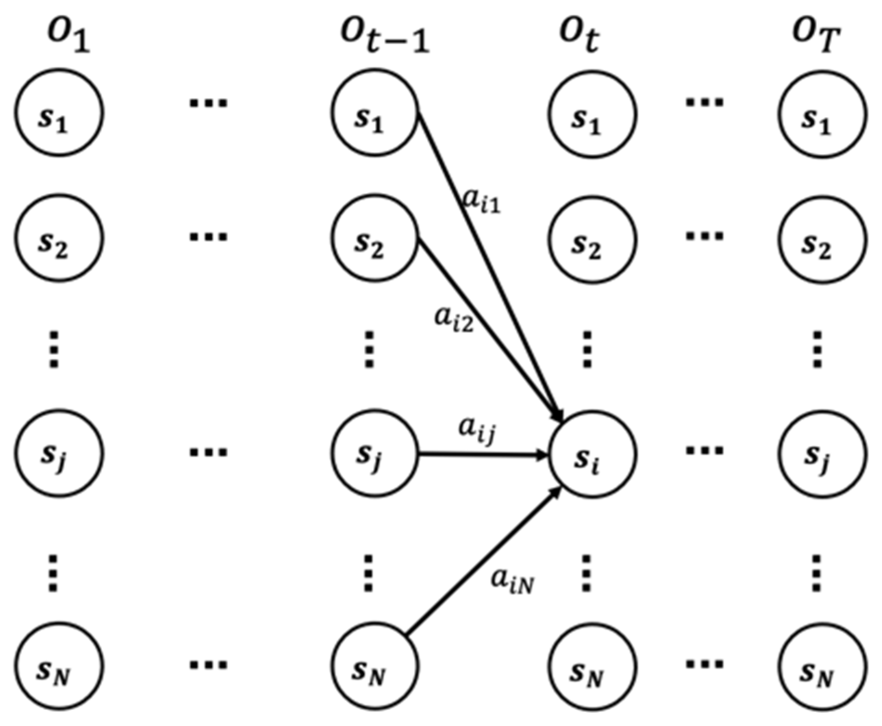
In HMM, the process of determining the sequence of latent or unobservable variables that correspond to a given sequence of observations is referred to as the decoding problem. To address this problem, the Viterbi algorithm is employed in HMMs. This algorithm utilizes dynamic programming principles to calculate the optimal path probabilities, thereby achieving a globally optimal solution. Specifically, the Viterbi algorithm recursively computes the optimal path probability at the current timestamp by considering previous probabilities, along with the state transition probability distribution and emission probability distribution. By comparing the probabilities of different paths, the path with the maximum probability is selected as the optimal path. The Viterbi algorithm generates the most probable state sequence for a given observation sequence by utilizing the constructed trellis. The Viterbi trellis is shown in Figure 2. Given observations and the HMM model , the optimal hidden state sequence can be found based on the Viterbi algorithm. is the set of hidden states, and represents the probability of transitioning from state to state .
The Viterbi algorithm works as follows:
- (1)
- Initialization. Initialize the algorithm by assigning initial values for the first hidden state based on the initial probability distribution and emission probability distribution.
- (2)
- Recursion. Iteratively compute the probabilities of all possible hidden state sequences up to a given GPS measurement .
- (3)
- Termination. Identify the final state by finding the sequence that maximizes the probability.
- (4)
- Backtracking. Trace back through the sequence to determine the most likely path of hidden states that led to the identified final hidden state.
- (5)
- Return the optimal hidden state sequence.
- (6)
- is the maximum probability of producing observation sequence when moving along a hidden state sequence and getting into state .
4. The Enhanced HMM for Map-Matching
4.1. Problem Statements
The initial state distribution plays a crucial role in the Viterbi algorithm for HMM in map-matching. The Markov property implies that the distribution of the current state depends on the distribution of the previous state, making the distribution of the initial states influential, especially for those states within a certain amount time in the early stage of navigation, despite the stationary distribution property. Traditionally, the uniform distribution is commonly used to specify the initial state distribution and the emission probability distribution is typically based solely on the distance between GPS measurements and road segments [13,26,27,39]. However, taking just the distance into account may be insufficient due to the large GPS error. We propose using a heuristic approach to determining the probability distribution of initial states. That is, given a pedestrian trajectory and a road network , the goal is to determine an initial state distribution of the HMM in order to find the most probable road segment for the initial GPS measurement .
HMM breaks can occur in many cases, such as when there are no road segments within the search area of a GPS measurement [13]. An open-field area such as a lawn field and an open square are good examples. The search area is a circular region of radius centered around a GPS measurement. Road segments covered by the search area of a GPS measurement are candidate roads for this GPS measurement. We propose adding a new hidden state in our HMM so that GPS measurements obtained while a person is traversing an open field can be matched to the new hidden state. In our experiment, the value of search area radius does not dynamically adapt to changes in the environment.
The problem definition of handling the open field traversal is defined as follows: Given a pedestrian trajectory traversing open fields and a road network , the goal is to represent an open field as a hidden state of the HMM and redefine the emission and transition probability distributions to improve the stability and accuracy of map-matching.
4.2. EHMM-P
This paper proposes an enhanced HMM in map-matching for pedestrians (EHMM-P) that can improve the performance of pedestrian navigations using the Viterbi algorithm in terms of map-matching accuracy based on heuristics. Our proposed method leverages a small number of GPS measurements during a short warm-up period to specify the initial state distributions. It also incorporates an additional open-field hidden state and introduces a new emission and transition probability distribution considering the preceding GPS measurements and other factors, i.e., distance difference, direction difference, and position difference. It then utilizes a human trajectory forecasting model that learns human mobility patterns to generate open-field trajectories that align with human behavior.
4.2.1. Probability Distributions of the Initial States
The probability distribution of initial states is usually defined by a uniform distribution, while the emission probability distribution is defined as a function based only on the distance between GPS measurements and road segments, as shown in Equation (2). It is clear that the probability of initial states would be unreliable due to the GPS error. We propose a new initial state distribution based on a small number of GPS measurements during a short warm-up period called calibration time that is a user-defined parameter. The GPS measurements , collected during are called calibration points. is the total number of calibration points collected during the calibration time . Calibration points are used to determine the probability density function for the initial states. From the work on the second-order HMM, we can understand that utilizing historical information more extensively is more beneficial for map-matching of the current GPS measurement [38,40]. Similarly, it is beneficial for map-matching of the initial GPS measurement when there are more correction points. In the experiment section, we will describe how to select an appropriate calibration time.
We acknowledge that human mobility is spatiotemporally continuous, with the current position depending on the preceding or even more distant locations. Therefore, how to utilize historical information at the current time is a question worthy of profound consideration. Diverging from conventional approaches like the second-order HMM that utilizes historical data, we performed a mapping of calibration points based on pedestrian movement patterns. We introduce the notion of an arrival point, which refers to the location on a road segment that a pedestrian is assumed to reach at a particular future time based on the current GPS location and a fixed walking distance. Each calibration point corresponds to an arrival point at the current time. The distance error between these arrival points and the real road segment is attributed to GPS error, known to follow a Gaussian distribution [13]. The probability of a road segment being in the initial state is higher than other road segments when arrival points are closer to that road segment. Subsequently, we will explain how to compute and use arrival points.
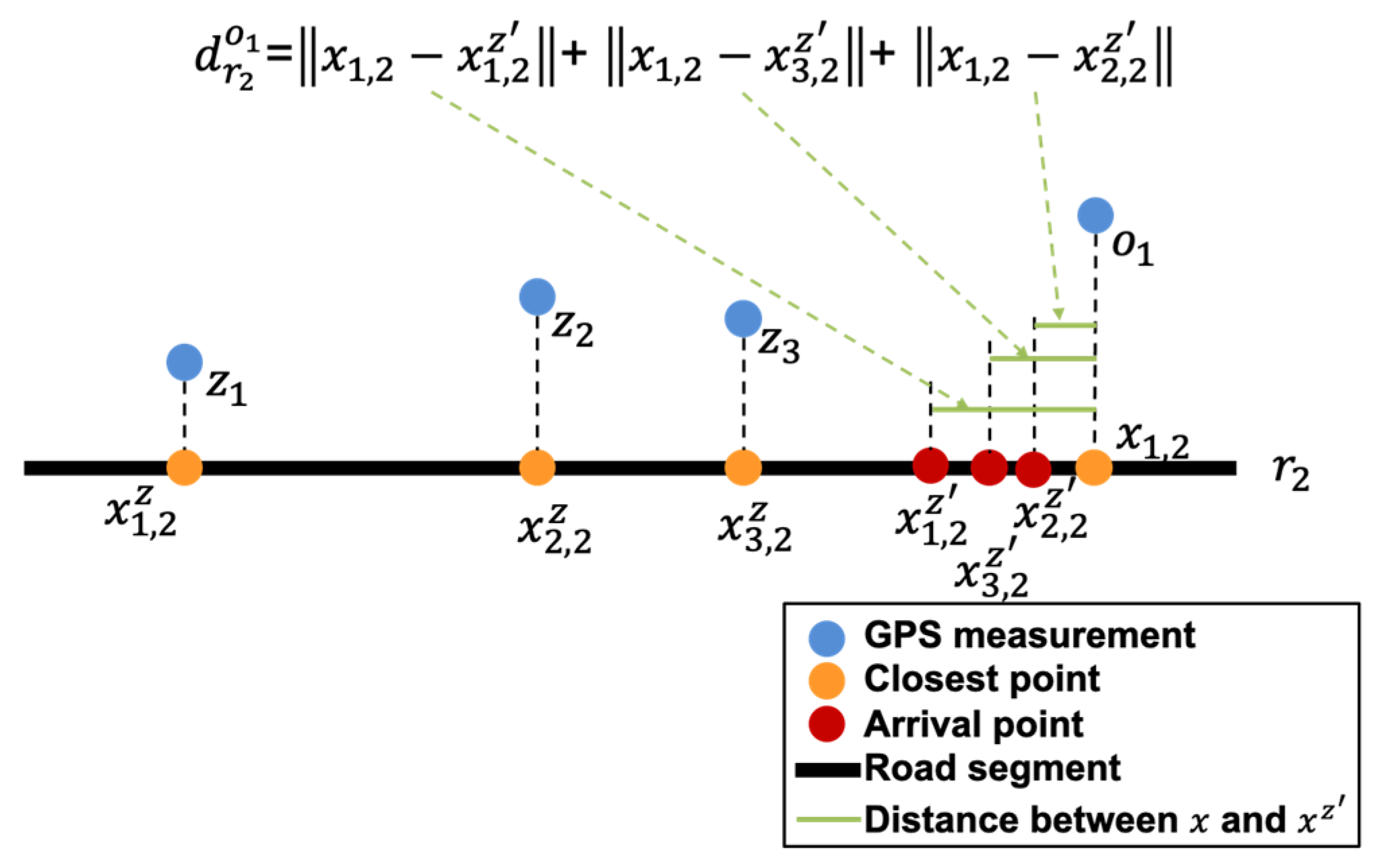
The position of an arrival point is determined by the location of a calibration point and the expected distance traveled along the route during the calibration time. The expected distance can be calculated by multiplying the time between the moment a calibration point is collected and the current time by the average speed , which can be estimated as
Figure 3 shows an illustration of where is the distance between calibration point and and , which was determined based on the experiments conducted as described in Section 5.2 A.
The on-route position of a calibration point is determined by computing the closest point on the route in order to obtain an arrival point. We define the , , as the closest point on road segment of calibration point . To distinguish the closest point of calibration points and the closest point of the first GPS measurement, we define , as the closest point on the road segment of the GPS measurement . We can then determine an arrival point for each calibration point by multiplying by the number of time steps between the calibration point and the initial GPS measurement . Each time step is separated by 1 sec according to 1 Hz GPS data collection frequency. is defined as the arrival point of . Figure 4 illustrates two scenarios of how to obtain the arrival points of calibration points along the road towards In Figure 4a, the closest point on road segment of calibration point , walking along road segment , will reach the arrival point after one time step, that is, at the initial time. The distance between and is , as indicated by the orange line. Similarly, will arrive at after two time steps. The length of the blue line is representing the distance between and . And, will arrive at after three time steps. The distance between and is denoted by the green line, with a length equal to . In Figure 4b, the closest point on road segment of calibration point , walking along road segment , will reach the arrival point after one time step, that is, at the initial time. The walking path is illustrated with the orange line and the length is . Similarly, , walking from road segments to , will arrive at after two time steps. The walking path is represented by the blue polyline, with a length of . And, , walking from road segments to and then to , will arrive at after three time steps. Represented by the green polyline, the walking path from to has a length of .
We introduce a distance component to the initial state probability, based on the total distance between the closest point of GPS measurement on road segment and arrival points , denoted as .
We define a new probability distribution for the initial states at the time of :
where is the summation of distance for candidate road segments.
Intuitively, takes on the largest value for the road segment on which the arrival points are closest to the closest point of the initial GPS measurement. Figure 5 illustrates an example where the arrival point of the calibration point, denoted by , indicates the on-road location that calibration point would reach at the initial time according to the average speed and is the sum of the distances from three arrival points to the closest points of on .
Consequently, the initial probability of the hidden states can be computed using
4.2.2. Emission and Transition Probability Distributions
As discussed earlier, conventional HMMs might incorrectly match GPS measurements on an open field to road segments. Therefore, a HMM needs to be enhanced to be capable of handling both open-field as well as non-open-field trajectories. In our enhanced HMM model, we represent an open-field as a special hidden state and redefine the emission and transition probability distributions to ensure the continuity and accuracy of map-matching.
Given GPS measurements as the observations, the set of hidden states is augmented by hidden state representing an open-field so that the new set of hidden states becomes .
The introduction of an open-field as a new hidden state requires adjustments to the emission and transition probability distributions of the conventional HMM. We propose new emission and transition probability distributions that leverage the preceding GPS measurements and the information between measurements and hidden states.
Emission Probability Distribution
Many HMMs for map-matching have adopted the approach proposed by [13] to design emission probabilities that road segments close to the GPS measurements are more likely to be the correct road segments. Intuitively, the emission probabilities are inversely proportional to the distance between the GPS measurement and the road segment. We adopt this idea and use the probability density function based on the distance between a GPS measurement and the closest points on the road segments as the new emission probability. However, when the state corresponds to an open field, the GPS measurement would not have the closest points on the road segments. Therefore, we use GPS measurement itself as a candidate position to replace the closest point on the road segment. In this case, the Gaussian probability density function based on GPS error reaches its maximum value, which is evidently incorrect. Thus, we introduce the so-called the total length factor to differentiate the probability depending on whether the state is in the open-field state or a road state. Intuitively, when there are many roads within the search area of a GPS measurement, it is more likely that the GPS measurement is on the road rather than on the open field. The GPS measurements on an open field may have few or no roads within the search area.
where is the length of the road segment within the search area, and is the parameter of the exponential distribution to be empirically determined. Figure 6 shows an example of . The red circle represents the search area at time . and are lengths of the road segments and within the search area for GPS measurement , while the lengths of are zero. The emission probability distribution is defined as
where is the standard deviation of Gaussian GPS noise. represents the Euclidean distance between the estimated position and GPS measurement . The estimated position is the closest point on that candidate road segment when the state corresponds to a road segment. When the state corresponds to an open field, the estimated position is , and the distance-based Gaussian distribution always yields the maximum value . In this case, is used to determine probabilities. The observation, , has the probability that can be observed from each of the hidden states. Therefore, we need to compute Equation (12) times, with each computation representing the probability of located in a specific state.
Transition Probability Distribution
The conventional transition probability assumes that the Euclidean distance between two GPS measurements is similar to the route distance between the two closest points for correct matching [13]. However, the difference between the Euclidean distance and the route distance, as described in Equation (4), cannot be determined in the case of an open-field location due to the lack of route distance. We propose new transition probabilities for four kinds of transition scenarios: (a) from a road segment to another road segment, (b) from a road segment to an open field, (c) from an open field to a road segment, and (d) remaining on an open field. The movement vector of a GPS measurement is defined as the average vector of a few preceding GPS measurements:
where is the number of preceding GPS measurements, and is the vector from to . Note that should be less than or equal to the number of calibration points . When , represents the vector between and . When , represents the vector between calibration and . In the Viterbi algorithm, the calculation of the transition probability can be performed starting from .
Using the movement vector found, three different probabilities can be obtained based on the three new attributes described below. These probabilities are then multiplied together to determine the transition probabilities.
- (1)
- Distance Difference
The difference between two distance values, i.e., the distance between the estimated positions at two consecutive time steps and the magnitude of the movement vector (we denote this quantity as ‘distance difference’ hereafter), is caused by GPS errors, which follow Gaussian distribution [13]. The probability distribution based on the distance difference is defined as
where is the standard deviation of Gaussian GPS noise. represents the estimated position of , and represents the estimated position of . In the case of a hidden state for a road segment, the estimated position should be the closest point of the current GPS measurement on the road segment. On the other hand, in the case of an open field, the estimated position would be the current GPS location. That is, represents the closest point on for GPS measurement when corresponds to road segment , whereas represents the GPS measurement when corresponds to an open field. represents the distance between two estimated positions, and . When one of the estimated positions is the GPS measurement itself, . Otherwise, , where denotes the route distance. is the difference between the magnitude of the movement vector and .
For each transition, the distance difference between two estimated positions and the magnitude of the movement vector will be computed. An example of the distance differences in each transition scenario is shown in Figure 7. Two blue points, and , represent GPS measurements. Two yellow points, and , represent estimated positions of GPS measurement and GPS measurement . is the distance between two estimated positions. A red arrow represents the movement vector. For each scenario, is calculated as described above. In Figure 7a, both hidden states correspond to road segments, from which we take the closest points on the roads as the estimated points and compute the route distance from to . In Figure 7b–d, each of them contains at least one hidden state corresponding to an open-field state, . Therefore, we use the GPS measurement itself as the estimated point to calculate the Euclidean distance between the two estimated points. The probabilities of all possible transitions need to be computed using Equation (14) within these four kinds of distance differences. Note, however, that it does not imply that probabilities only include four values. For instance, in Figure 7a, could correspond to any road segment, {}, resulting in time computations for this scenario. Similarly, Figure 7b,d each require time computations, while scenario Figure 7c requires only one computation. The smaller distance difference will reach the higher probability .
- (2)
- Direction Difference
We consider the angle between the movement vector and the vector of estimated positions at two consecutive time steps as the direction difference. As mentioned before, represents the estimated position of , and represents the estimated position of . The notion of the direction difference is made based on the assumption that humans tend to maintain their original direction of movement. The direction difference is defined as
where is the radian value of the angle between and from to . For each transition, we calculate the direction difference. In order to make this value large, when the direction difference is small, the reciprocal of is used with 1 added in the denominator to prevent the error of division by zero, as given in Equation (15).
The direction differences in four kinds of state transition scenarios are shown in Figure 8. For different hidden states, corresponding to different estimated points and , we use the vector with the starting point and the end point as . The angle between and the movement vector is .
- (3)
- Position Difference
The heuristic method to compute the initial state probabilities based on arrival points described in Section 4.2.1 can be adopted here to differentiate the probabilities of state sequences. At time , we can determine the maximum probability of a state sequence ending with hidden state of time . We then obtain a sub-sequence from time to , denoted as , …, = , . The sequence is stored in matrix . The estimated position of hidden state serves as the starting point, moving in the direction and distance of . The state sequence would reach the arrival position at time . The direction of this arrival point is obtained based on the state at time and, walking the distance , it reaches the arrival point of GPS measurement at time , where is the movement vector mentioned before. We calculate the distance between the arrival point and the estimated position of . Subsequently, the summation of distances between the estimated position of the GPS measurement and these arrival points is calculated. Like considering only the distance between two GPS measurements, if there were no GPS errors, the arrival point would coincide with the estimated position of . The GPS error introduces a difference between an arrival point and the estimated position of . Thus, the sum of distances follows a Gaussian distribution. It is defined as
where represents the distance between the estimated position of and the arrival point of . The transition probability is high when the summation of distances is small. The arrival point in each state transition scenario is shown in Figure 9. As described before, when the state is road segment, the estimated point is the closest point on the road. When the state is an open area, the estimated point is the GPS measurement itself. Figure 9a is the estimated point of and moves along the road direction for one time step, reaching the arrival point . Figure 9b–d are their respective corresponding estimated points at time ; taking as the velocity and walking for a time step, they will reach their arrival point at Time . represents the distance between the estimated position of and the arrival point of . Note that only is shown in this example.
Based on the probability distributions associated with the three new attributes described above, the new transition probability distribution can be defined as
As mentioned in [13], while some of the GPS errors may not be strictly based on Gaussian distribution, both their experiment and ours have demonstrated its effectiveness.
4.2.3. Algorithm
We define as the maximum probability of the state sequence of the length that ends in state . is defined as the state of states sequences with maximum probability at state and time , which will be saved in the matrix . When we compute the third part of transition probability, , we can obtain the sub-sequence from . The and are defined as follows:
After (18) and (19) are updated recursively, the probability of the optimal state sequence and the end state of the optimal state sequence are defined in (20) and (21), respectively.
As a result, the Viterbi algorithm finds the sequence of states with the maximum probability product via backtracking . The optimal path corresponding to the given observation sequence is obtained by concatenating the optimal states in the optimal state sequence. The optimal state sequence could include both road segments and open-field states. Each open-field state at a different timestamp is associated with the GPS measurement at that timestamp.
With the introduction of open fields as a hidden state and the incorporation of multiple factors in the proposed HMM, the computational cost increases. The algorithm proposed in this research still has the same time complexity as conventional HMM-based map-matching. The complexity of the Viterbi algorithm is for conventional HMM. We add a new hidden state, the open-field state, for which the complexity of our proposed EHMM-P is . Our approach can achieve the computation of approximately 1000 GPS points per second, similar to the reference work, where Viterbi was also employed to search for the optimal path of HMM for map-matching [41]. Algorithm 1 shows the summary of the proposed EHMM-P. Table 1 shows the summary of notations.
| Algorithm 1 EHMM-P |
| Inputs: GPS trajectory ; Road network Outputs: Matched road segments and open-field trajectory 1. Initialization: For each do 2. 3. For each do 4. For each and do 5. Recursion: 6. Termination: 7. Backtracking: For do 8. Initialize and as empty lists 9. For in do 10. If is a road segment do 11. 12. Else 13. Return and |
4.2.4. Trajectory Prediction in Open-Fields Based on Human Mobility Patterns
The EHMM-P method determines which GPS measurements should be matched to an open-field based on the probability distributions. A pre-trained model called Y-net is utilized for the GPS measurements identified as open-field measurements to generate open-field trajectories that align with human behavior [42]. Y-net can predict scene-compliant multimodal human trajectories within the open-field based on scene semantics and human mobility patterns using a few open-field measurements identified via EHMM-P and a destination measurement (i.e., the last location identified via EHMM-P before exiting the open-field). We select the trajectory that is closest to the GPS trajectory determined via EHMM-P from the multiple trajectories predicted using Y-net as the trajectory predicted using EHMM-P+Y-net. This approach aligns with human mobility patterns and does not deviate from the overall pedestrian trajectory.
5. Experiments
A series of comparative experiments using field data was conducted to evaluate the proposed EHMM-P. The EHMM-P comprises new probabilities of initial states, new emission, and transition probability distribution. Comparisons were made between the conventional HMM and Behr’s method in order to evaluate the performance of the proposed method [2,35]. Behr’s approach involves creating a grid on the open field and utilizing Dijkstra’s algorithm to find the path with minimum energy consumption.
The experimental setup involved utilizing a dataset collected from real-world scenarios, which included GPS measurements and corresponding ground truth locations. The map-matching of each method was evaluated from various perspectives to assess their performance. This section begins with an introduction to the collection and pre-processing of the dataset, followed by a series of comparative experiments. Finally, the performance of each method is analyzed and discussed.
5.1. Data Collection and Data Preprocessing
The pedestrian walking trajectory data used in the experiment were collected from pedestrians carrying GPS-equipped mobile phones at a sampling frequency of 1 Hz as they walked along pre-defined routes in the campus. We computed the ground truth location based on the distance and angle data measured between current location and landmark position. The road network data were .shp format with nodes and links. The ground truth locations and corresponding road segments were manually measured and recorded.
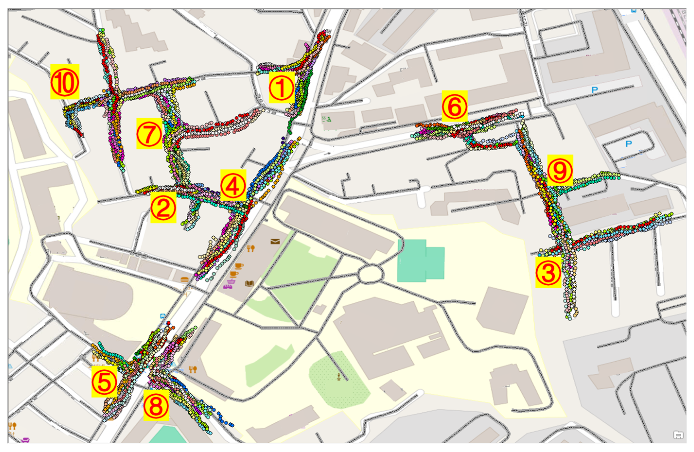
To evaluate the proposed EHMM-P, we collected two pedestrian walking trajectory datasets. Dataset I was collected to evaluate the proposed probability distributions of the initial states at ten intersections near the campus, denoted by the yellow markers in Figure 10. The area is characterized by dense architecture, with buildings not exceeding 20 m in height. For each intersection, we planned five paths around each interaction to contain various scenarios. We walked for approximately thirty seconds while collecting GPS measurements, repeating it five times on each path. Dataset I comprised 7700 GPS measurements in total. We were allowed to go straight or make turns through the intersections.
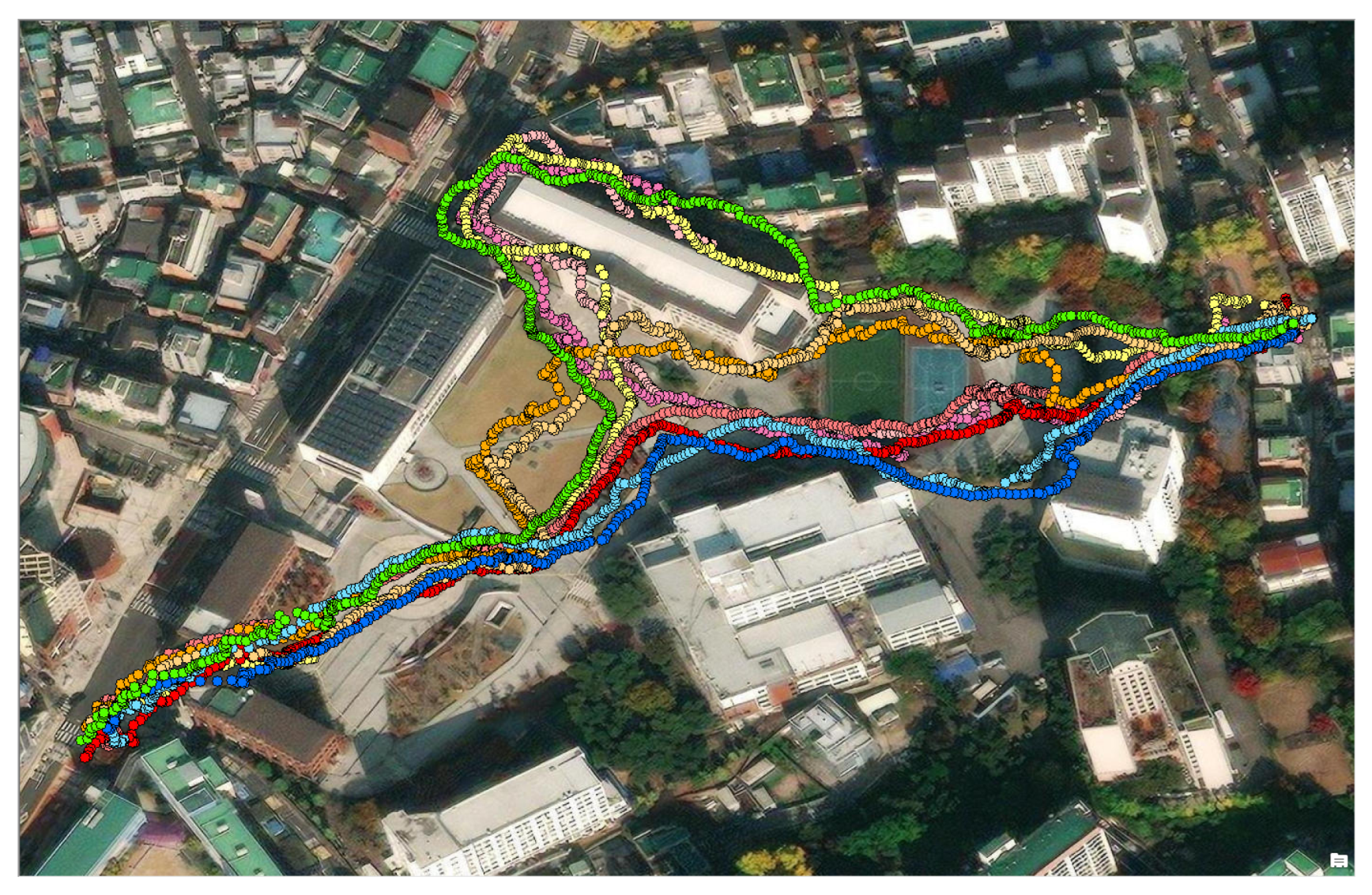
Dataset II was primarily collected within the campus and comprised extended trajectories traversing open fields where buildings are sparse. It encompassed five pre-defined routes, each of which was traversed twice in the opposite direction, as shown in Figure 11. Each trajectory contains at least two open fields. Comprehensive information regarding Dataset II is provided in Table 2.
5.2. Results and Discussion
In this chapter, we compared the outcomes obtained by utilizing various calibration times for map-matching. We conducted a comparative assessment of the accuracy achieved using different methods for map-matching on trajectories that traverse open fields. The map-matching accuracy is defined as the ratio of correctly matched GPS measurements to the total number of GPS measurements with corresponding ground truth road segments, as given in Equation (22):
where is the number of GPS measurements correctly matched on road segments, and is the total number of ground truth points on road segments. We also use a performance metric called ‘route mismatched fraction’, , proposed by [13] to measure the matching accuracy. This fraction is the sum of the lengths of mismatched road segments, denoted as , and the lengths of unmatched road segments, denoted as , divided by the total length of the correct route, denoted as . The route mismatch fraction is only avaliable for the locations on the road segments. We compute the Fréchet distance using Behr’s method to evaluate the prediction of open-field locations. The Fréchet distance is a standard distance measure for curves to describe the similarity between two paths. Given two sequences of points , and , and a monotone path , the discrete Fréchet distance between the two sequences, is the distance
- A.
- Performance Evaluation of Proposed Method for Initial Map-Matching
We compare the influence of probability distributions of initial states based on the traditional and the proposed methods in terms of the accuracy of entire map-matching. We use the distance-based emission and transition probability distribution suggested by Newson and Krumm in both methods on Dataset I [13].
The accuracy of map-matching for the initial single GPS measurements was assessed across various calibration time lengths. Figure 12 displays the map-matching accuracy in various calibration times ranging from 4 to 8 s. For the trade-offs between insufficient duration for obtaining a movement vector and the adverse impact on user experience, we selected a calibration period of 4 to 8 s in our experiments. The conventional HMM remains unaffected by the calibration time. Fluctuations in HMM results occur because different initial points are selected when using different calibration times, leading to variations in the initial point matching results and impacting the map-matching accuracy. The results indicate that the map-matching accuracy of EHMM-P outperforms that of the traditional method within the 4 to 8 s calibration time. The escalating calibration time correlates with an improved matching accuracy for EHMM-P, suggesting that a greater number of calibration points yields more accurate results. Nevertheless, longer calibration times correlate with increased user waiting times, which must be strictly controlled for optimal user experience in practical applications. To strike a balance between response time and map-matching accuracy, we adopted a 4 s calibration time in the subsequent experiments. In practice, the calibration time can be set as an adjustable parameter, permitting users to select shorter calibration times for faster outcomes or longer calibration times for higher map-matching accuracy.
Figure 13 displays the map-matching results of intersection 4 on Dataset I, utilizing probabilities of initial states based on the traditional and the proposed methods. The red lines are road segments. The blue and green circles are the closest points of the road segment as the map-matching results of the traditional and proposed method for visualization, respectively. The yellow and orange circles are the GPS measurements and ground truth locations, respectively. The first four GPS measurements were used as the calibration points for our model and GPS measurement 4 is the initial point. The conventional HMM matched all these GPS measurements to the right-side road segment, which is the most probable sequence of states predicted by the Viterbi algorithm. Our method computes the initial probability based on Equation (10). As shown, our proposed method maps GPS measurements to the left-side road segment that the ground truth on. The initial matching of GPS measurement 4 significantly influences the matching results of all subsequent GPS measurements.
- B.
- Performance Evaluation of Map-matching
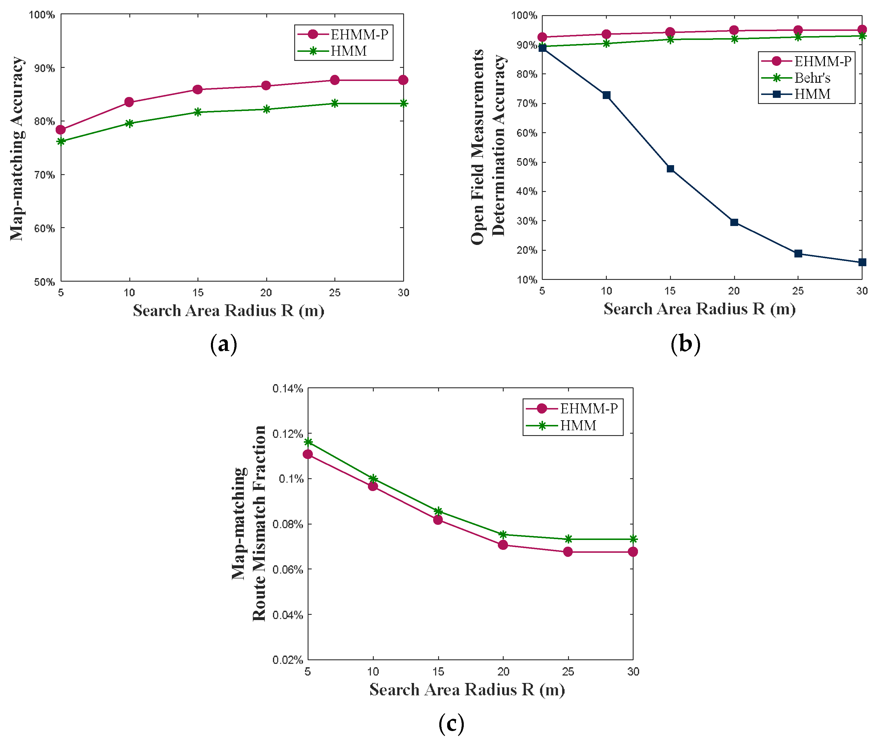
Next, a comparison of three different methods for map-matching was conducted: (i) the conventional HMM, (ii) Behr’s method, and (iii) the proposed EHMM-P. We examined the performance of these methods using different search radii since the size of the search radii has a considerable amount of impact on the performance of models. With an increase in the search radius, the number of candidate road segments also grows. In the case of conventional HMMs, explicit identification of open-field GPS measurements is not carried out. GPS measurements without candidate road segments within the search area are considered as open-field GPS measurements in conventional HMMs.
We measured the map-matching accuracy, as shown in Figure 14a, for various values of search radii in dense urban areas of Dataset I. When the search radius is 5 m, the accuracies of conventional HMM and EHMM-P are lower than those of other radii as the small search area with a lack of candidate road segments leads to numerous points on the road being directly classified as open-field points. With the increase in the search radius, there is an increased probability of matching points with substantial errors on the road to road segments, resulting in an enhancement of the matching accuracy of conventional HMM and EHMM-P. Figure 14b illustrates the accuracy of identifying open-field GPS measurements using three different methods on Dataset II. As mentioned above, the HMM will match GPS measurements to road segments within the search area as the radius increases, leading to a decrease in the determination rate of open-field measurements. Behr’s method generates a grid road network over open fields, allowing GPS measurements from such areas to be matched onto the created road network, resulting in higher accuracy with a larger search radius. As the search radius increases to 25 m, it leads to an increased likelihood of matching to road segments because of the total length factor, thereby reducing the accuracy of identification of EHMM-P. In our scenario, as the radius increases, the accuracy of EHMM-P remains higher than other methods. Figure 14c presents the route mismatch fraction proposed by [13] of the three methods on the entirety of Dataset I. As the radius increases, some locations with large errors can match to the correct roads that are farther away, which could reduce the magnitude of the route mismatch fraction. Our proposed EHMM-P achieves better map-matching performance than conventional HMM in dense urban areas, excluding open fields.
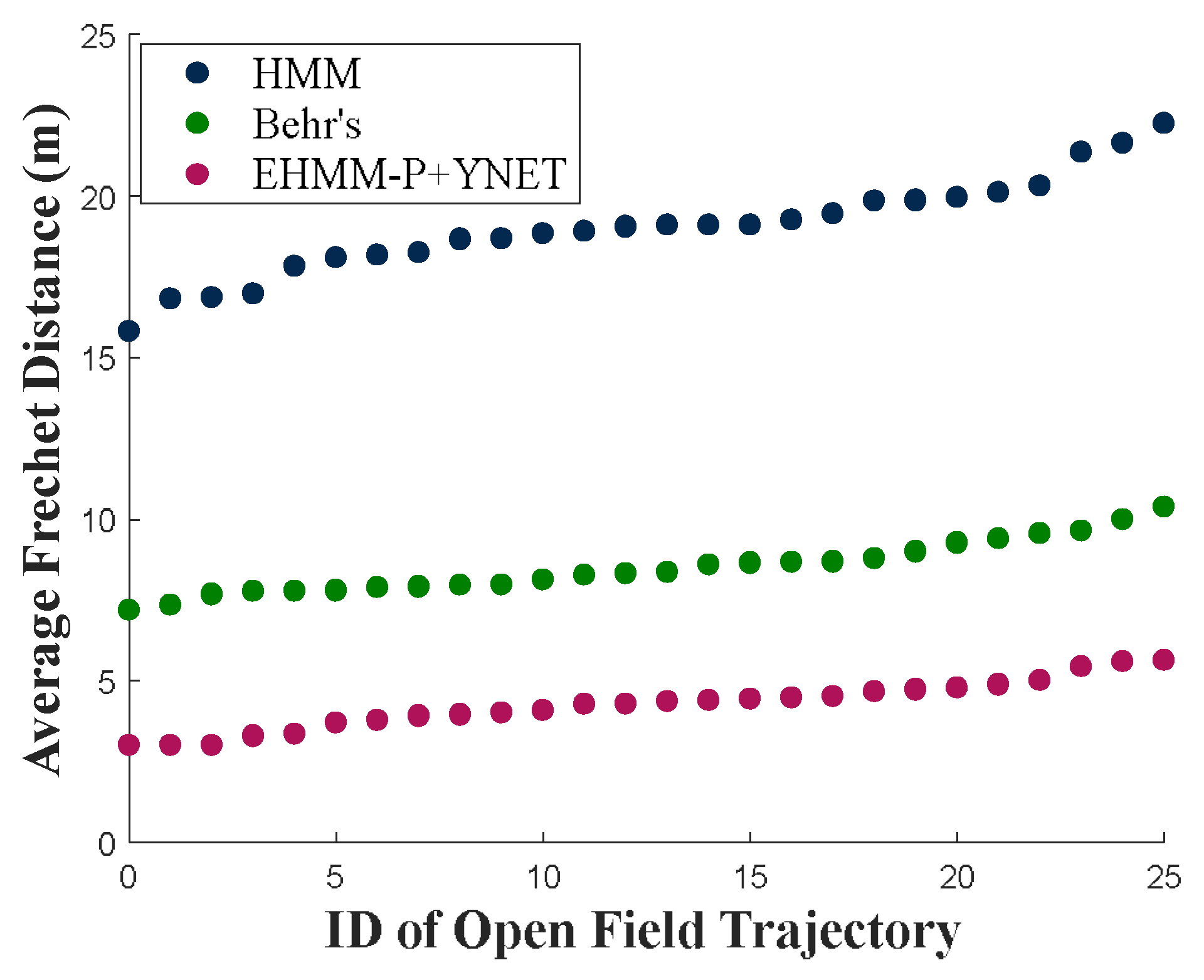
The performance of open-field predicted trajectories is evaluated using the average Fréchet distance, as shown in Figure 15. Behr’s method outputs the prediction of trajectories for those GPS measurements that are included in the tessellation. Our EHMM-P method with Y-net could predict a trajectory of open-field measurements. As the determination accuracy increases, Behr’s method and EHMM-P correctly match more locations in open fields, resulting in a reduced discrepancy between the predicted trajectory and the actual trajectory compared to when locations are incorrectly matched to roads. EHMM-P+Y-net considers human mobility patterns, which can predict the trajectory closer to the ground truth path with a small Fréchet distance.
Additionally, we computed the average reductions in positioning error for the entire trajectories via map-matching on Datasets I and II, and presented them in Table 3.
Figure 16 illustrates prediction results using the three methods, i.e., (a) conventional HMM, (b) Behr’s method, and (c) EHMM-P, respectively. To provide a clearer demonstration of the prediction of each method, we use the closest point on the road segment matched to GPS measurements as the visualized prediction results, instead of displaying the matched road segments; for the points matched to the open-field, we draw the trajectory predicted using EHMM-P+Y-net. The map-matching results consider not just whether the GPS measurements are matched to the correct road segment but whether open-field GPS measurements are mapped onto road segments as well. The traditional HMM always matches GPS measurements to road segments if they exist within the search range. As we can see clearly in Figure 16a, all GPS measurements are matched to corresponding roads. On the other hand, the method proposed by Behr and EHMM-P can identify open-field points. In Figure 16b, tessellation of the open-field (light blue area) is used in path matching in the Behr’s method (pink polyline). In this case, for ground truth locations from location 198 to location 249 in the open-field, EHMM-P and Behr’s detected locations 200 to 250 and locations 205 to 243 as open-field locations are used, respectively. Although EHMM-P incorrectly matches points 198 and 199 to the road segment, all points prior to location 198 are correctly matched to the ground truth road segment. In contrast, Behr’s method incorrectly matches points prior to 198 to the wrong road segment. Similarly, as the trajectory exits the open-field, EHMM-P can identify more GPS measurements to the correct hidden states, whereas Behr’s method mismatches some open-field measurements to the wrong hidden states. Compared to Figure 16b,c, it can be observed that our method achieves a higher map-matching accuracy and detection rate of open-field GPS measurements.
- C.
- Human Behavior-Based Trajectory Prediction in Open-fields
Y-net is used to generate open-field trajectories that align with human behavior for the open-field locations determined using EHMM-P [42]. The input consists of the GPS measurements in the open-fields and Google Earth maps, while the output is the prediction. The pink polyline and green circles in Figure 16b,c illustrate the trajectories generated using Behr’s method and EHMM-P+Y-net, respectively. EHMM-P determines GPS measurements starting from location 200 as the open-field point, with location 200 to 204 inputted to the Y-net for predicting subsequent pedestrian trajectories. The top 20 trajectories with the highest probability are generated by the Y-net. The trajectory with the smallest average distance to the GPS measurement trajectory was selected using EHMM-P+Y-net. By incorporating learned human behavior patterns and environmental information from Google Earth images, the model captures the complexity of pedestrian motion, resulting in predicted trajectories that closely resemble actual human walking patterns and effectively avoid obstacles.
6. Conclusions
This paper proposes an enhanced HMM for map-matching in pedestrian navigation. EHMM-P focuses on improving the accuracy of map-matching for pedestrians, specifically targeting the issues of persistent map-matching error due to the large localization error in the initial phase of map-matching and lack of handling in the state of open-field traversal. EHMM-P introduces a new probability distribution for the initial states of HMM, which is established using a limited set of GPS data collected during a warm-up period. The HMM model is adapted to incorporate an additional hidden state for open-field scenarios, accompanied by redefined emission and transition probability density functions. Furthermore, an existing Y-net model trained on human mobility patterns is employed to predict human trajectories in open fields, selecting the most similar trajectory as the EHMM-P+Y-net prediction, which most likely aligns with human behavior for GPS measurements.
Extensive comparative experiments using field GPS data validate the performance of EHMM-P. The results confirm its effectiveness in improving pedestrian map-matching accuracy compared to traditional HMM and Behr’s methods. EHMM-P demonstrates good generalization across different datasets and performs well in diverse scenarios. The limitation of our proposed method is that it is not truly a real-time method since it requires a short period of time to collect the calibration points to compute the initial state probability and dynamic adaptive behavior of the map-matching method under various GPS/positioning environments is not considered in the proposed method. And, the transition and emission probabilities may not be based on the Gaussian distribution for some GPS measurements. A machine learning approach may be considered as an alternative to improve the accuracy in unstable GPS environments. Future research directions include leveraging deep learning methods to further enhance the performance of EHMM-P, incorporating a wider range of human behavioral patterns for trajectory prediction and exploring inverse reinforcement learning to improve the probabilistic representation of HMM.
Author Contributions
Conceptualization, methodology, S.M., P.W. and H.L.; software, S.M.; validation, formal analysis, investigation, resources S.M., P.W. and H.L.; data curation, S.M.; writing—original draft preparation, S.M. and P.W.; writing—review and editing, S.M., P.W. and H.L.; visualization, S.M. and P.W.; supervision, H.L.; project administration, H.L.; funding acquisition, H.L. All authors have read and agreed to the published version of the manuscript.
Funding
This research was supported by the MSIT, Korea under the National Program for Excellence in SW supervised by the IITP (No. 2017-0-00096) and the Research Grant of Kwangwoon University in 2022.
Data Availability Statement
The data presented in this study are available on request from the corresponding author. The data are not publicly available due to privacy.
Conflicts of Interest
The authors declare no conflicts of interest.
References
- Siriaraya, P.; Wang, Y.; Zhang, Y.; Wakamiya, S.; Jeszenszky, P.; Kawai, Y.; Jatowt, A. Beyond the shortest route: A survey on quality-aware route navigation for pedestrians. IEEE Access 2020, 8, 135569–135590. [Google Scholar] [CrossRef]
- Kim, Y.H.; Choi, M.J.; Kim, E.J.; Song, J.W. Magnetic-map-matching-aided pedestrian navigation using outlier mitigation based on multiple sensors and roughness weighting. Sensors 2019, 19, 4782. [Google Scholar] [CrossRef]
- Bang, Y.; Kim, J.; Yu, K. An Improved Map-Matching Technique Based on the Frechet Distance Approach for Pedestrian Navigation Services. Sensors 2016, 16, 1768. [Google Scholar] [CrossRef]
- Hashemi, M.; Karimi, H.A. A weight-based map-matching algorithm for vehicle navigation in complex urban networks. J. Intell. Transp. Syst. 2016, 20, 573–590. [Google Scholar] [CrossRef]
- Maaref, M.; Kassas, Z.M. Ground vehicle navigation in GNSS-challenged environments using signals of opportunity and a closed-loop map-matching approach. IEEE Trans. Intell. Transp. Syst. 2019, 21, 2723–2738. [Google Scholar] [CrossRef]
- Lai, C.; Zhang, M.; Cao, J.; Zheng, D. SPIR: A secure and privacy-preserving incentive scheme for reliable real-time map updates. IEEE Internet Things J. 2019, 7, 416–428. [Google Scholar] [CrossRef]
- An, Q.; Feng, Z.; Chen, S.; Huang, K. A green self-adaptive approach for online map matching. IEEE Access 2018, 6, 51456–51469. [Google Scholar] [CrossRef]
- Ahmed, M.; Karagiorgou, S.; Pfoser, D.; Wenk, C. A comparison and evaluation of map construction algorithms using vehicle tracking data. GeoInformatica 2015, 19, 601–632. [Google Scholar] [CrossRef]
- Ding, Z.; Yang, B.; Guting, R.H.; Li, Y. Network-Matched Trajectory-Based Moving-Object Database: Models and Applications. IEEE Trans. Intell. Transp. Syst. 2015, 16, 1918–1928. [Google Scholar] [CrossRef]
- Priambodo, B.; Ahmad, A.; Kadir, R.A. Predicting Traffic Flow Propagation Based on Congestion at Neighbouring Roads Using Hidden Markov Model. IEEE Access 2021, 9, 85933–85946. [Google Scholar] [CrossRef]
- Chen, Z.; Jiang, Y.; Sun, D. Discrimination and prediction of traffic congestion states of urban road network based on spatio-temporal correlation. IEEE Access 2019, 8, 3330–3342. [Google Scholar] [CrossRef]
- Wei, X.; Li, J.; Feng, K.; Zhang, D.; Li, P.; Zhao, L.; Jiao, Y. A Mixed Optimization Method Based on Adaptive Kalman Filter and Wavelet Neural Network for INS/GPS During GPS Outages. IEEE Access 2021, 9, 47875–47886. [Google Scholar] [CrossRef]
- Newson, P.; Krumm, J. Hidden Markov map matching through noise and sparseness. In Proceedings of the 17th ACM SIGSPATIAL International Conference on Advances in Geographic Information Systems, Seattle, WA, USA, 4–6 November 2009; pp. 336–343. [Google Scholar]
- Forney, G.D. The Viterbi algorithm. Proc. IEEE 1973, 61, 268–278. [Google Scholar] [CrossRef]
- Abdallah, F.; Nassreddine, G.; Denoeux, T. A Multiple-Hypothesis Map-Matching Method Suitable for Weighted and Box-Shaped State Estimation for Localization. IEEE Trans. Intell. Transp. Syst. 2011, 12, 1495–1510. [Google Scholar] [CrossRef]
- Chambers, E.; Fasy, B.T.; Wang, Y.; Wenk, C. Map-matching using shortest paths. ACM Trans. Spat. Algorithms Syst. (TSAS) 2020, 6, 1–17. [Google Scholar] [CrossRef]
- Liu, X.; Liu, K.; Li, M.; Lu, F. A ST-CRF map-matching method for low-frequency floating car data. IEEE Trans. Intell. Transp. Syst. 2017, 18, 1241–1254. [Google Scholar] [CrossRef]
- Alrassy, P.; Jang, J.; Smyth, A.W. OBD-Data-Assisted Cost-Based Map-Matching Algorithm for Low-Sampled Telematics Data in Urban Environments. IEEE Trans. Intell. Transp. Syst. 2022, 23, 12094–12107. [Google Scholar] [CrossRef]
- Huang, Z.; Qiao, S.; Han, N.; Yuan, C.; Song, X.; Xiao, Y. Survey on vehicle map matching techniques. CAAI Trans. Intell. Technol. 2021, 6, 55–71. [Google Scholar] [CrossRef]
- Hu, Y.; Lu, B. A Hidden Markov Model-Based Map Matching Algorithm for Low Sampling Rate Trajectory Data. IEEE Access 2019, 7, 178235–178245. [Google Scholar] [CrossRef]
- Hansson, A.; Korsberg, E.; Maghsood, R.; Nordén, E. Lane-level map matching based on HMM. IEEE Trans. Intell. Veh. 2021, 6, 430–439. [Google Scholar] [CrossRef]
- Choi, K.; Suhr, K.; Jung, J.H.G. Map-Matching-Based Cascade Landmark Detection and Vehicle Localization. IEEE Access 2019, 7, 127874–127894. [Google Scholar] [CrossRef]
- Lee, Y.J.; Suhr, J.K.; Jung, H.G. Map Matching-Based Driving Lane Recognition for Low-Cost Precise Vehicle Positioning on Highways. IEEE Access 2021, 9, 42192–42205. [Google Scholar] [CrossRef]
- Ma, S.; Lee, H. Improving positioning accuracy based on self-organizing map (SOM) and inter-vehicular communication. Trans. Emerg. Telecommun. Technol. 2019, 30, e3733. [Google Scholar] [CrossRef]
- Zhang, L.; Cheng, M.; Xiao, Z.; Zhou, L.; Zhou, J. Adaptable Map Matching Using PF-net for Pedestrian Indoor Localization. IEEE Commun. Lett. 2020, 24, 1437–1440. [Google Scholar] [CrossRef]
- Ren, M.; Karimi, H.A. Movement pattern recognition assisted map matching for pedestrian/wheelchair navigation. J. Navig. 2012, 65, 617–633. [Google Scholar] [CrossRef]
- Jagadeesh, G.R.; Srikanthan, T. Online Map-Matching of Noisy and Sparse Location Data with Hidden Markov and Route Choice Models. IEEE Trans. Intell. Transp. Syst. 2017, 18, 2423–2434. [Google Scholar] [CrossRef]
- Goh, C.Y.; Dauwels, J.; Mitrovic, N.; Asif, M.T.; Oran, A.; Jaillet, P. Online map-matching based on hidden markov model for real-time traffic sensing applications. In Proceedings of the 15th International IEEE Conference on Intelligent Transportation Systems, Anchorage, AK, USA, 16–19 September 2012; pp. 776–781. [Google Scholar]
- Osogami, T.; Raymond, R. Map matching with inverse reinforcement learning. In Proceedings of the 23rd International Joint Conference on Artificial Intelligence, Beijing, China, 3–9 August 2013; pp. 2547–2553. [Google Scholar]
- Chao, P.; Hua, W.; Mao, R.; Xu, J.; Zhou, X. A survey and quantitative study on map inference algorithms from gps trajectories. IEEE Trans. Knowl. Data Eng. 2020, 34, 15–28. [Google Scholar] [CrossRef]
- Shen, Z.; Du, W.; Zhao, X.; Zou, J. DMM: Fast map matching for cellular data. In Proceedings of the 26th Annual International Conference on Mobile Computing and Networking, London, UK, 21–25 September 2020; pp. 1–14. [Google Scholar]
- Perttula, A.; Leppäkoski, H.; Kirkko-Jaakkola, M.; Davidson, P.; Collin, J.; Takala, J. Distributed Indoor Positioning System with Inertial Measurements and Map Matching. IEEE Trans. Instrum. Meas. 2014, 63, 2682–2695. [Google Scholar] [CrossRef]
- Zampella, F.; Ruiz, A.R.J.; Granja, F.S. Indoor Positioning Using Efficient Map Matching, RSS Measurements, and an Improved Motion Model. IEEE Trans. Veh. Technol. 2015, 64, 1304–1317. [Google Scholar] [CrossRef]
- Zhong, Y. HMM Map Matching for Trajectories in City Areas with Multipath Errors. Master’s Thesis, Eindhoven University of Technology, Eindhoven, The Netherlands, 2021. [Google Scholar]
- Behr, T.; van Dijk, T.C.; Forsch, A.; Haunert, J.H.; Storandt, S. Map Matching for Semi-Restricted Trajectories. In Proceedings of the 11th International Conference on Geographic Information Science (GIScience 2021), Online, 27–30 September 2021. [Google Scholar]
- Boissonnat, J.-D.; Devillers, O.; Teillaud, M.; Yvinec, M. Triangulations in CGAL. In Proceedings of the 16th Annual Symposium on Computational Geometry, Hong Kong, China, 12–14 June 2000; pp. 11–18. [Google Scholar]
- Sasaki, Y.; Yu, J.; Ishikawa, Y. Road Segment Interpolation for Incomplete Road Data. In Proceedings of the 2019 IEEE International Conference on Big Data and Smart Computing (BigComp), Kyoto, Japan, 27 February–2 March 2019; pp. 1–8. [Google Scholar]
- Ding, X.; Fan, H.; Gong, J. Towards generating network of bikeways from Mapillary data. Comput. Environ. Urban Syst. 2021, 88, 101632. [Google Scholar] [CrossRef]
- Fu, X.; Zhang, J.X.; Zhang, Y. An Online Map Matching Algorithm Based on Second-Order Hidden Markov Model. J. Adv. Transp. 2021, 2021, 9993860. [Google Scholar] [CrossRef]
- Salnikov, V.; Schaub, M.T.; Lambiotte, R. Using higher-order Markov models to reveal flow-based communities in networks. Sci. Rep. 2016, 6, 23194. [Google Scholar] [CrossRef] [PubMed]
- Koller, H.; Widhalm, P.; Dragaschnig, M.; Graser, A. Fast hidden Markov model map-matching for sparse and noisy trajectories. In Proceedings of the 2015 IEEE 18th International Conference on Intelligent Transportation Systems, Gran Canaria, Spain, 15–18 September 2015; IEEE: Piscataway, NJ, USA, 2015; pp. 2557–2561. [Google Scholar]
- Mangalam, K.; An, Y.; Girase, H.; Malik, J. From goals waypoints & paths to long term human trajectory forecasting. In Proceedings of the IEEE/CVF International Conference on Computer Vision (ICCV), Montreal, BC, Canada, 11–17 October 2021; pp. 15233–15242. [Google Scholar]
Figure 1.
The illustration of route distance and Euclidean distance between two GPS measurements, by courtesy of Newson and Krumm [13]. The dashed arrows represent distances.
Figure 1.
The illustration of route distance and Euclidean distance between two GPS measurements, by courtesy of Newson and Krumm [13]. The dashed arrows represent distances.

Figure 2.
The Viterbi trellis for computing the optimal sequence through the hidden states.

Figure 3.
An illustration of the average speed .

Figure 4.
An illustration of how to determine arrival points. The length of the blue line is representing the distance between and . The length of the green line is representing the distance between and . (a,b) represent different possible walking paths.
Figure 4.
An illustration of how to determine arrival points. The length of the blue line is representing the distance between and . The length of the green line is representing the distance between and . (a,b) represent different possible walking paths.

Figure 5.
An illustration of computing .

Figure 6.
An example of total length factor .

Figure 7.
The distance differences in four kinds of state transition scenarios: (a) state transition from road segment to road segment ; (b) state transition from road segment to open field ; (c) state transition from open field to open field ; and (d) state transition from open field to road segment .

Figure 8.
The direction differences in four kinds of state transition scenarios: (a) state transition from road segment to road segment ; (b) state transition from road segment to open field ; (c) state transition from open field to open field ; and (d) state transition from open field to road segment .

Figure 9.
The arrival points in four kinds of state transition scenarios: (a) state transition from road segment to road segment ; (b) state transition from road segment to open field ; (c) state transition from open field to open field ; and (d) state transition from open field to road segment .
Figure 9.
The arrival points in four kinds of state transition scenarios: (a) state transition from road segment to road segment ; (b) state transition from road segment to open field ; (c) state transition from open field to open field ; and (d) state transition from open field to road segment .


Figure 10.
Dataset I: GPS measurements collected in a dense urban area with 10 intersections. The terms in Korean represent the names of buildings and places. The circles are GPS measurements.
Figure 10.
Dataset I: GPS measurements collected in a dense urban area with 10 intersections. The terms in Korean represent the names of buildings and places. The circles are GPS measurements.


Figure 11.
Dataset II: ten trajectories on campus. The terms in Korean represent the names of buildings and places.
Figure 11.
Dataset II: ten trajectories on campus. The terms in Korean represent the names of buildings and places.


Figure 12.
Map-matching accuracy of traditional and our proposed probabilities of initial states with various calibration time length on Dataset I.
Figure 12.
Map-matching accuracy of traditional and our proposed probabilities of initial states with various calibration time length on Dataset I.

Figure 13.
Visualization of map-matching results on the Dataset I using the probabilities of initial states based on the traditional (blue) and the proposed (green) methods.
Figure 13.
Visualization of map-matching results on the Dataset I using the probabilities of initial states based on the traditional (blue) and the proposed (green) methods.

Figure 14.
(a) Map-matching accuracy. (b) Open-field measurement determination accuracy. (c) Route mismatch fraction for various values of search radii (m).
Figure 14.
(a) Map-matching accuracy. (b) Open-field measurement determination accuracy. (c) Route mismatch fraction for various values of search radii (m).

Figure 15.
Average Fréchet distance of traditional HMM, Behr’s method, and proposed EHMM-P method for various values of search radii R (m) on Dataset II.
Figure 15.
Average Fréchet distance of traditional HMM, Behr’s method, and proposed EHMM-P method for various values of search radii R (m) on Dataset II.

Figure 16.
Visualization of map-matching results on Dataset II based on the (a) conventional HMM (blue), (b) Behr’s method (pink), and (c) EHMM-P (green). The GPS trajectory is represented as yellow points and the ground truth trajectory is represented as orange points. The red lines are road segments.


Table 1.
Summary of Notations.
| Notations | Descriptions |
|---|---|
| GPS measurement | |
| Road segment | |
| Open-field hidden state | |
| The set of hidden states | |
| The probability of the optimal state sequence | |
| The end state of the optimal state sequence | |
| The standard deviation of GPS measurements | |
| The parameter of the exponential distribution | |
| -th road segment within the search area | |
| Matched road segment sequence | |
| Matched open-field sequence |
Table 2.
Detailed information of each path.
| Path ID | No. of GPS Measurements | No. of Open-Field GPS Measurements |
|---|---|---|
| 1 | 910 | 317 |
| 2 | 794 | 320 |
| 3 | 1442 | 641 |
| 4 | 917 | 489 |
| 5 | 767 | 374 |
| Total | 4830 | 2141 |
Table 3.
Average reductions in positioning error.
| Method | HMM | Behr’s Method | EHMM-P |
|---|---|---|---|
| Reduced Error (m) | 1.02 | 2.35 | 4.63 |
Disclaimer/Publisher’s Note: The statements, opinions and data contained in all publications are solely those of the individual author(s) and contributor(s) and not of MDPI and/or the editor(s). MDPI and/or the editor(s) disclaim responsibility for any injury to people or property resulting from any ideas, methods, instructions or products referred to in the content. |
© 2024 by the authors. Licensee MDPI, Basel, Switzerland. This article is an open access article distributed under the terms and conditions of the Creative Commons Attribution (CC BY) license (https://creativecommons.org/licenses/by/4.0/).
Share and Cite
MDPI and ACS Style
Ma, S.; Wang, P.; Lee, H. An Enhanced Hidden Markov Model for Map-Matching in Pedestrian Navigation. Electronics 2024, 13, 1685. https://doi.org/10.3390/electronics13091685
AMA Style
Ma S, Wang P, Lee H. An Enhanced Hidden Markov Model for Map-Matching in Pedestrian Navigation. Electronics. 2024; 13(9):1685. https://doi.org/10.3390/electronics13091685
Chicago/Turabian StyleMa, Shengjie, Pei Wang, and Hyukjoon Lee. 2024. "An Enhanced Hidden Markov Model for Map-Matching in Pedestrian Navigation" Electronics 13, no. 9: 1685. https://doi.org/10.3390/electronics13091685
Note that from the first issue of 2016, this journal uses article numbers instead of page numbers. See further details here.