Abstract
Machine vision systems use industrial cameras’ digital sensors to collect images and use computers for image pre-processing, analysis, and the measurements of various features to make decisions. With increasing capacity and quality demands in the electronic industry, incoming quality control (IQC) standards are becoming more and more stringent. The industry’s incoming quality control is mainly based on manual sampling. Although it saves time and costs, the miss rate is still high. This study aimed to establish an automatic defect detection system that could quickly identify defects in the gold finger on printed circuit boards (PCBs) according to the manufacturer’s standard. In the general training iteration process of deep learning, parameters required for image processing and deductive reasoning operations are automatically updated. In this study, we discussed and compared the object detection networks of the YOLOv3 (You Only Look Once, Version 3) and Faster Region-Based Convolutional Neural Network (Faster R-CNN) algorithms. The results showed that the defect classification detection model, established based on the YOLOv3 network architecture, could identify defects with an accuracy of 95%. Therefore, the IQC sampling inspection was changed to a full inspection, and the surface mount technology (SMT) full inspection station was canceled to reduce the need for inspection personnel.
1. Introduction
Machine vision systems use industrial cameras’ digital sensors to collect images and use computers for image pre-processing, analysis, and the measurements of various features to make decisions. Machine vision systems include a host computer, an image capture card, an image processor, an image camera (such as closed-circuit television (CCTV) and microlens), a lighting source (such as LED or infrared light), an image display, and other components. A machine vision system for industrial inspection includes a programmable logic controller (PLC), a PC-based controller (PC-base), a servo motion machine, and other components.
1.1. State of the Art in Defect Detection
Defect detection, a critical facet of quality control, has undergone a transformative journey from conventional methods to the integration of sophisticated machine learning (ML) approaches. This subsection delves into the historical context and contemporary landscape of defect detection, offering insights into the evolution of methodologies and the recent surge in ML-driven advancements.
1.1.1. Traditional Defect Detection Methods
In the earlier stages of manufacturing and quality assurance, defect detection primarily relied on manual inspection and rule-based systems. Visual examination, human expertise, and manual quality control processes were the cornerstones of defect identification. While effective to a certain extent, these methods faced inherent human subjectivity, scalability, and speed challenges. As industries evolved and production scales increased, the limitations of traditional approaches became more apparent.
Traditional defect detection methods refer to established techniques employed for identifying and inspecting defects in various materials or products. These methods have been in use for a considerable period and often involve manual or rule-based automated approaches. A breakdown of key aspects is presented as follows:
- (1)
- Magnetic Particle Inspection, Penetrant Inspection, Eddy Current, etc.: Chen et al. [1] mentioned techniques like magnetic particle inspection, penetrant inspection, and eddy current. These methods rely on physical phenomena to reveal defects in materials, such as cracks or discontinuities.
- (2)
- Manual Inspection: traditional defect detection often involves a manual inspection by human operators or experts. This approach relies on visual examination and expertise to identify defects in materials or products.
- (3)
- Pattern Recognition and Image Processing: Some traditional methods leverage basic computer visions, pattern recognition, and image processing techniques for defect detection. These methods may include algorithms designed to identify specific patterns associated with defects.
- (4)
- Application-Specific Approaches: Depending on the industry and application, traditional defect detection methods vary. For instance, Bhattacharya and Cloutier [2] discussed fabric defect detection methods, which could involve specific techniques tailored for textiles.
Traditional methods have paved the way for modern approaches, such as machine vision and deep learning. While they are effective, traditional methods may have limitations in handling complex defects or require more manual effort. The advent of advanced technologies aims to overcome these limitations and enhance the accuracy and efficiency of defect detection.
1.1.2. Machine Learning-Based Defect Detection
The advent of machine learning (ML) ushered in a new era for defect detection, presenting a paradigm shift in automated quality control. ML algorithms, particularly those based on deep learning principles, showcased unparalleled capabilities in discerning intricate patterns and anomalies within manufacturing processes. These advancements not only enhanced the speed and accuracy of defect identification but also paved the way for the exploration of complex datasets. Recent years have witnessed the ascendancy of state-of-the-art ML models in defect detection. Notable approaches include the Faster Region-Based Convolutional Neural Network (FRCNN), RetinaNet, and You Only Look Once (YOLO). These models leverage convolutional neural networks (CNNs) and object detection techniques to achieve exceptional mean average precision (mAP) scores. A comparison with traditional methods highlights the superior performance of ML-based models, particularly in scenarios involving low-resolution images.
Machine Learning (ML)-based defect detection has witnessed significant advancements, shaping the state of the art in various domains. Noteworthy contributions include:
- (1)
- Selective Laser Sintering Defect Detection: Westphal et al. [3] proposed a convolutional neural network (CNN)-based method for defect detection in selective laser sintering, showcasing the application of ML in additive manufacturing.
- (2)
- Software Defect Detection: McMurray [4] explored ML-based software defect detection, emphasizing the importance of selecting appropriate ML algorithms and models to enhance software defect prediction.
- (3)
- Segmentation-Based Deep Learning Architecture: A segmentation-based deep-learning architecture is presented for surface anomaly detection [5]. This methodology demonstrates the effectiveness of deep learning in identifying and segmenting defects.
- (4)
- Transportation Infrastructure Defect Detection: Sui et al. [6] conducted a state-of-the-art review of ML applications in transportation infrastructure defect detection, using ground penetrating radar (GPR) in particular.
- (5)
- Visual Defect Detection using CNN: Jha et al.’s [7] survey of current approaches in visual defect detection focused on CNNs and pixel-level segmentation techniques.
- (6)
- Root Cause Analysis: Papageorgiou [8] provided a systematic review of ML methods for root cause analysis, utilizing techniques such as Principal Component Analysis and Dynamic Time Warping.
In recent years, the field of defect detection technologies has witnessed significant advancements, particularly in the application of machine learning and deep learning techniques. Several studies have explored innovative approaches to enhance the accuracy and efficiency of defect detection processes. Bhattacharya and Cloutier [9] proposed a streamlined deep-learning framework for the efficient detection and classification of manufacturing defects on printed circuit boards (PCBs). Chen and Xie [10] proposed a new method for detecting defects on circuit boards in the fields of optical sensors and optical devices. The motivation behind this research is the need for extremely high precision and performance in applications such as fiber optic communication, optical computing, biomedical devices, and high-performance computing devices. Tabernik et al. [5] proposed a segmentation-based deep-learning architecture specifically designed for the detection and segmentation of surface anomalies, focusing on the domain of surface-crack detection. Soomro et al. [11] proposed a robust printed circuit board (PCB) classification system using computer vision and deep learning to aid in sorting e-waste for recycling. Volkan and Akgül [12] proposed a defect detection system for printed circuit boards (PCBs) using machine learning and deep learning algorithms. The system aims to accurately produce PCBs and minimize error rates by detecting various defects such as missing holes, mouse bites, open circuits, shorts, spurs, and spurious copper. Huang et al. [13] proposed an application of deep learning, specifically three integrated models for automatic defect detection in printed circuit boards (PCBs) using automatic optical inspection (AOI) technology. Huang et al. [14] proposed a predictive model using a decision tree to analyze electronics manufacturing data and predict the circuit board assembly process yield. Huang et al. [15] proposed a machine vision system for intelligent decision analysis to evaluate solder ball cracking and its interface in Ball Grid Array (BGA) package components. Ray and Mukherjee [16] introduced a hybrid approach that helped in producing zero-defect PCB by detecting the defects. Li et al. [17] proposed a self-adaptive method that collected error-related data from the automated optical inspection edge, retrained the artificial intelligence model on the server with these data, and deployed the updated model back to the edge. Çelik et al. [18] suggested an automated inspection system using vision-based technology for identifying pixel defects on LCD panels.
1.2. Research Motivation
The conventional manual sampling method employed for incoming quality control (IQC) in the electronics industry, though cost-effective, presents notable shortcomings. The high miss rate associated with manual sampling poses a significant risk to the subsequent manufacturing processes and the overall quality of the final product. This inadequacy results in the need for additional, often labor-intensive, second manual sampling inspections to ensure product quality, leading to increased operational costs and time consumption. The motivation for this research arises from the imperative to overcome these limitations. By adopting machine vision systems, we aim to revolutionize IQC standards and address the deficiencies of the manual sampling approach. Machine vision systems offer the potential for a more accurate and comprehensive inspection of raw materials, reducing the miss rate and enhancing overall production efficiency. The integration of industrial cameras, image processors, and advanced analytics in machine vision systems promises to provide a reliable and automated solution, ensuring not only improved quality control but also increased production capacity. Our research endeavors to optimize IQC processes in the electronics industry, aligning with the growing demands for heightened production capacity and quality standards.
1.3. Research Purpose
This study proposes the development of an automated defect detection system for efficiently identifying faults on the gold finger of printed circuit boards (PCBs) based on manufacturer-defined standards. The primary objective is to enhance the efficiency and accuracy of incoming quality control procedures, potentially replacing or augmenting manual inspections. Leveraging deep learning networks, this research aims to establish a self-learning system by training the model on a diverse dataset. Continuous automatic updates during the training process will optimize image processing techniques and deductive reasoning calculations, contributing to the establishment of efficient fault determination standards. The study evaluates the system’s performance against manual inspection methods, focusing on speed, accuracy, and adaptability to various defect types. Additionally, there is an exploration of opportunities for human-in-the-loop integration to ensure collaborative decision-making between the automated system and human expertise. The anticipated outcomes include the development of a robust automated defect detection system with the potential to revolutionize incoming quality control in the electronics manufacturing industry.
1.4. Research Process
First, status analysis was carried out according to the incoming quality control specifications and equipment, and the defect characteristics were clearly defined. Second, the image acquisition equipment and shooting process were confirmed, after which defect images were collected for the training samples. Then, Labeling Master software (version 1) was used to mark the position and category of defects on a single image, and the YOLO Version 3 (You Only Look Once Version 3; YOLOv3) and Faster R-CNN (faster regions with CNN features) algorithms were used to train and test the model. Finally, the accuracy of the confusion matrix was employed to compare the results from the above two methods to find the one with the higher accuracy for building the defect detection system.
Our reason for employing YOLOv3 stems from its well-established reputation for achieving a harmonious blend of accuracy and speed, rendering it particularly adept for real-time applications. Despite the existence of newer iterations, the pragmatic choice of YOLOv3 is underpinned by its proven robustness and reliability. Its widespread adoption across diverse industrial applications provides a wealth of documentation and community support, ensuring a stable and comprehensively understood foundation for our defect detection system. Also, drawing upon the scholarly investigations conducted by Nepal and Eslamiat [19] and Ge et al. [20], it was discerned that YOLOv3 exhibited a superior Frames Per Second (FPS) performance in comparison to both YOLOv4 and YOLOv5l. As for the inclusion of Faster R-CNN in our experimentation, it was motivated by its effectiveness in precisely identifying object boundaries and managing intricate feature representations. While newer models offer incremental improvements, Faster R-CNN remains a benchmark for object detection tasks, known for its comprehensibility, established performance, and versatility in handling diverse datasets. Our rationale for selecting YOLOv3 and Faster R-CNN revolves around striking a balance between harnessing cutting-edge advancements and ensuring the dependability and interpretability essential for industrial applications, aligning closely with the specific requirements and constraints of our defect detection system.
2. Quality Control and Image-Based Defect Classification
This study used printed circuit boards in memory storage products to analyze the testing process status. Each panel contained five printed circuit boards (PCBs), and each PCB contained 144 golden fingers, as shown in Figure 1. In our defect detection study, the decision to utilize a set of fingers instead of individual finger images sliced was grounded in a comprehensive consideration of several factors. First and foremost, this choice aimed to provide a more realistic representation of defect occurrences in industrial settings, where defects often manifest across a group of neighboring fingers rather than isolated to individual ones. This approach enhances the authenticity of our study by aligning with the actual conditions of defect occurrence in PCBs. Moreover, analyzing a set of fingers allows for a richer contextual understanding of defect detection, as defects may exhibit patterns or correlations across neighboring fingers. This consideration becomes crucial for accurately identifying subtle variations and anomalies. From a practical standpoint, working with sets of fingers streamlines the training and testing processes, reducing the dataset size while maintaining the required complexity for a robust machine-learning model. This choice aligns with common industrial practices, where inspections are frequently performed on groups or batches of components rather than individual units. Overall, the use of a set of fingers enhances the efficiency, practicality, and real-world applicability of our defect detection system.
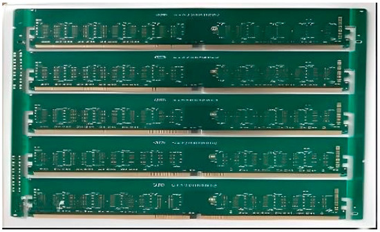
Figure 1.
Display of a panel comprising five PCBs (each PCB is intricately designed with 144 golden fingers).
The first IQC sampling inspection was carried out after the raw PCB material was placed into the material, following MIL-STD-105E specifications, for which 0.4 is the acceptable standard. Then, a second total test was performed. Both tests were performed manually with a microscope at a magnification of 10–15×. The inspected PCB entered the surface mount technology (SMT) manufacturing process and was then sent to the test station for a memory test (MT) by direct personnel. Next, it was sent to the quality memory test station (quality memory test; QMT) for sampling inspection by indirect personnel. Finally, packing and a full inspection were carried out to complete the final product’s final quality control (FQC), after which it was sent to the warehouse.
2.1. Defect Categories
The IQC defect classification criterion currently considers the causes of defects; however, the defect detection system developed in this study was trained and learned from the image appearance characteristics of defects. Therefore, the original IQC defect categories (seven categories in total) were redefined as the following machine vision defect categories (five categories in total): dent, foreign material (FB), foreign material (between) (FBTW), scratch and poor gold finger size (PGF). The appearance characteristics of each defect category are shown in Figure 2 and illustrated as follows:
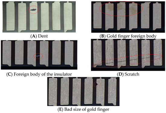
Figure 2.
Appearance characteristics of each gold finger defect category.
- (1)
- Dent: irregularly shaped flaws appearing in patches on the golden fingers, distinguished by significant color variations compared to the standard golden appearance (refer to Figure 2A).
- (2)
- Gold Finger Foreign Material: imperfections resembling the color of the gold finger itself (refer to Figure 2B).
- (3)
- Foreign Material (Between): foreign particles adhering to the insulator between two adjacent golden fingers (refer to Figure 2C).
- (4)
- Scratch: linear abrasions, particularly strip scratches (refer to Figure 2D).
- (5)
- Poor Gold Finger Size: deviations in both the shape and size of the gold finger, as depicted in Figure 2E.
2.2. Image Acquisition Method Confirmation and Defect Image Collection
In this study, an industrial camera was used with fly capture image acquisition software, and a telocentric lens was used with an external light source to control the image brightness. The model, specifications, and erection entity of the image-fetching device are shown in Table 1. The scope of the image acquisition in this study is shown in Figure 3. Each image contained six golden fingers. The image acquisition process was as follows:

Table 1.
Image acquisition equipment model and specifications.
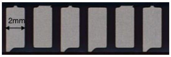
Figure 3.
Gold finger image range.
- (1)
- The PCB was placed on the shooting platform;
- (2)
- The industrial camera was fixed on the X-Y moving axis and automatically moved to the initial shooting position set by the computer;
- (3)
- The camera remained stationary for five seconds to allow the photographer to capture and archive the image;
- (4)
- The camera was moved to the next shooting range for image fetching. When the five-plate PCB fetching was completed, the inspector removed the PCB from the platform.
3. YOLOv3 Model Training
In this study, a YOLOv3 deep learning network was used to build a defect detection system. Its network architecture, model training, and bounding box prediction are described below.
3.1. Network Infrastructure
YOLOv3 uses the residual network (ResNet-53) and combines low-level and high-level defect information to solve the gradient vanishing problem. The residual network contained 53 convolutional layers and was called Darknet-53. In addition, feature pyramid networks (FPNs) were used to improve the prediction ability of the model for features with small defects [21]. In our study, Darknet-53 was created as part of the YOLOv3 model architecture for defect detection. The architecture of Darknet-53 involves the use of a residual network (ResNet) with 53 convolutional layers. This design was adopted to address the gradient vanishing problem by combining low-level and high-level defect information. The incorporation of feature pyramid networks (FPNs) further enhanced the model’s prediction ability for features with small defects.
The training process of YOLOv3, which includes Darknet-53, consisted of several key steps. Notably, the residual network was initialized with weights that were either randomly set or obtained from pre-training for subsequent fine-tuning. The model then underwent training to optimize its ability to detect defects, considering factors such as learning rate, anchor frame size, and loss functions. The loss function, detailed in Equation (2) in this paper, encompasses various components, including the confidence score and object detection, contributing to the overall training process.
3.2. YOLOv3 and Darknet-53: Advancements and Applications
This study on defect detection, particularly utilizing the YOLOv3 model with the Darknet-53 architecture, contributes to the broader field of machine learning fault detection in the following ways:
- (1)
- Architectural Advancements: Our research introduces Darknet-53, a residual network with 53 convolutional layers, as a key component of the YOLOv3 model. This architectural innovation aims to overcome challenges such as gradient vanishing by effectively combining low-level and high-level defect information. Darknet-53’s design is rooted in the well-established principles of ResNet and is further empowered by feature pyramid networks (FPNs). This contributes to the evolving landscape of neural network architectures for improved fault detection.
- (2)
- Effective Feature Extraction: Leveraging the principles of ResNet within Darknet-53 enhances the model’s capability for comprehensive feature extraction. The integration of FPN complements this by addressing the prediction challenges associated with small defective features. Our approach aligns with recent trends in ML fault detection, emphasizing the significance of robust feature extraction methods to enhance model accuracy and reliability.
- (3)
- Practical Application in Defect Detection: Our research is not solely theoretical but addresses a practical concern—defect detection. By implementing the YOLOv3 model with Darknet-53, we aim to provide a solution that is applicable in real-world scenarios. This aligns with the broader shift in ML fault detection research towards developing practical, deployable models that can be effectively utilized across various industries and domains.
3.3. Model Training
The training process of YOLOv3 consisted of five steps as follows: (1) input the images and training parameters, such as the learning rate and anchor frame size; (2) specify the weights of the randomly initialized network or input the weights from the pre-training for adjustment; and (3) use Equation (1) to calculate the output dimension of the image. In this step, the input image is first divided into S × S grids, and the model detects whether there are defective features within each grid. If the coordinates of a feature center fall within a grid, the model makes a feature prediction based on the dimension information of the grid. Next, B bounding boxes are formed using the central coordinates of each grid as the center, and the unique bounding boxes are retained after filtering according to the object score for specific categories. Five parameters of each boundary box are determined by the model, which are the central coordinates (x, y), width (W), height (H), and confidence. The model then predicts the probabilities of C categories for each grid. The variable “C” corresponds to the number of categories or classes that the YOLOv3 model is trained to recognize and detect. The definition of these categories is task-specific and determined by the objectives of our defect detection system. The categorization process involves annotating the training dataset with labels corresponding to different classes, ensuring that the model can distinguish between these predefined categories during training. The choice and definition of these categories are crucial steps in tailoring the model to the specific requirements of the application.
In step 4, Equation (2) calculates the loss value, which can be continuously updated and decreased with the training process. Finally, the iteration is completed when the loss value no longer decreases, and the model training is over.
where is the loss weight of the boundary box containing defects (); is the loss weight of the bounding box without defects (); indicates whether the defective center falls on grid i and if yes, the value is 1; otherwise, it is 0. Furthermore, denotes whether the jth bounding box in grid is responsible for this defect and if yes, the value is 1; otherwise, it is 0. Also, represents whether the jth bounding box in grid i is not responsible for this defect and if yes, the value is 1; otherwise, it is 0. means that the image is divided into S × S grids; B is the number of boundary boxes predicted by the grid (YOLOv3 is set to 3); is the offset from the grid coordinates to the real feature box coordinates; , is the offset from the grid coordinates to the predicted bounding box coordinates; is the anchor box to the real characteristics of the frame’s width and the size of the high scale; , is the size scaling of the width and height of the predicted bounding box; is the true features box in grid i’s confidence; is the confidence of the bounding box in grid i; for the actual grid belongs to the category of probability; and is the probability of predicting that grid i belongs to category .
3.4. Training Model Detection
First, the intersection over union (IoU) is calculated using Equation (3) for the defect position marked by the input image, i.e., the overlap rate between boundary box A and ground truth B. IoU is a measure of the overlap between the predicted bounding box and the ground truth. It is calculated as the ratio of the intersection area to the union area of the two boxes. The higher the IoU, the more accurate the prediction. In our study, the IoU score serves as a crucial metric for evaluating the localization performance of our defect detection model on printed circuit boards (PCBs). The IoU measures the overlap between predicted and actual defect positions, providing a key indicator of accuracy in localization. Our analysis consistently revealed high IoU scores across diverse defect scenarios, demonstrating the model’s robust capability in precisely delineating defect boundaries. Instances of lower IoU scores were carefully scrutinized to understand localization challenges. Given the significance of accurate defect localization in industrial quality control, where spatial precision is paramount, our findings affirmed the practical utility of our defect detection system in ensuring both the identification and precise location of anomalies on PCBs.
Then, Equation (4) is used to calculate the confidence, which indicates whether the bounding box contains features as well as the accuracy of the feature location. The confidence score is calculated based on the product of the following two components: the probability of the presence of an object (Pr(Object)) and the intersection over union (IoU) of the predicted bounding box with the ground truth. Pr(Object) represents the probability that an object is present within the predicted bounding box. It is equal to 1 if the bounding box contains features (defects, in this case) and 0 otherwise. The confidence score indicates how confident the model is in its prediction. Higher confidence scores suggest a stronger belief that the bounding box accurately contains the specified object. Then, Equation (5) is used to calculate the object score of a specific category, which represents the probability that the predicted bounding box can be attributed to this type of feature, namely, the accuracy. The confidence score is then compared with the preset threshold value. If the confidence score is less than the threshold value, the boundary box is filtered. If the remaining boundary box has the maximum confidence score, the final feature category and position of the model are provided.
where, if the bounding box contains features, Pr(object) is 1; otherwise, Pr(object) is 0.
where the Pr(|Object) for the prediction of the grid characteristics belongs to the category of .
3.5. Bounding Box Prediction
The learning goal of YOLOv3 is to scale , , and the confidence of the grid coordinates from the real ground truth to , , and the width and height of the real ground truth by the preset anchor box. These five values are used to obtain information about the bounding box according to the formula of the bounding box. The learning process is shown in Figure 4, in which the red frame is the preset anchor frame, and the green box is the real feature box. For coordinate translation, the solid red box is first translated to the dotted red box using Equations (6) and (7), and then the dotted red box is scaled to the green box according to Equations (7) and (8), in which (), , are the center coordinates, width, and height of the real feature box, respectively, and (cx, cy) is the upper-left coordinate of the grid.
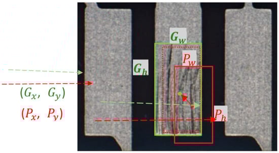
Figure 4.
YOLOv3 training process diagram.
Next, , , , and are substituted into Equations (10)–(12) to predict the information of the bounding box in which (), , and are the center coordinates, width, and height of the predicted boundary box, respectively; is an S-shaped growth curve function (Sigmoid function), which is intended to control the offset value between [0, 1] to prevent excessive offset; () is the upper-left coordinate of the grid; and and are the width and length of the preset anchor box, respectively. The prediction diagram of the bounding box is shown in Figure 5 [22].
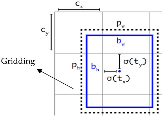
Figure 5.
Boundary box prediction diagram.
4. Faster R-CNN Model Training
In this study, the Faster R-CNN deep learning network was used to construct a defect detection system. Its network architecture, model training, and bounding box prediction are described below.
4.1. Network Infrastructure
The Faster R-CNN network architecture includes inception net, region proposal networks (RPN), and the region of interest pooling (ROI Pooling), as shown in Figure 6. Among them, the inception network extracts features through the structure of the broadened network to generate feature maps so that the training model can obtain more detailed defect feature information.
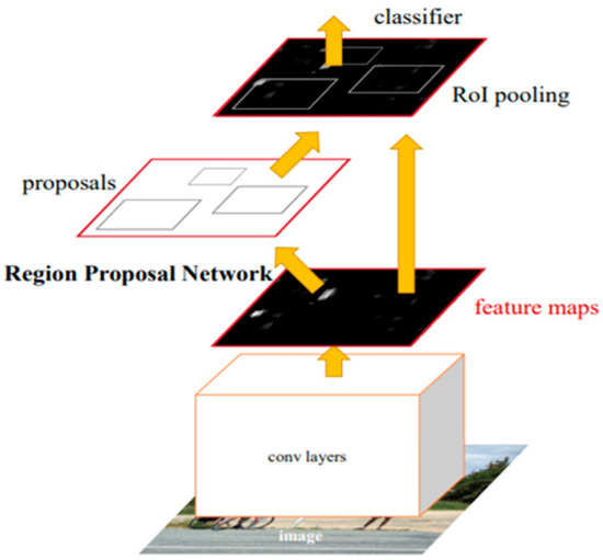
Figure 6.
Faster R-CNN framework.
4.2. Model Training
The Faster R-CNN training process consists of seven steps as follows: (1) input the image and training parameters; (2) use the inception network to extract features; (3) use the RPN network to generate the candidate box; (4) adjust the candidate box to a specific size in the ROI pooling layer; (5) use IoU to determine which defect category the candidate box belongs to and then correct the position of the candidate box; (6) use Equation (14) to calculate the loss value , which is continuously updated and decreases with the training process; and (7) when the loss value is no longer reduced, the iteration is completed and the model training is over.
where i is the defect category and is used to predict whether the bounding box contains this kind of flaw. If yes, the value is 1; otherwise, it is 0. is the predicted offset and size scaling of the bounding box by the anchor box; and are the loss weights, and their value is set by the number of bounding boxes, which is generally 256. refers to whether the real feature box contains class I defects, which, if “Yes” is 1, otherwise, it is 0. for the anchor box and the real characteristics of the frame’s actual offset and size scaling, R is the smooth L1 function, such as Equation (15), of which is three.
4.3. Boundary Box Prediction
Faster R-CNN inputs candidate boxes to the classification layer and bounding box regression layer for classification and position correction. In the classification layer, Faster R-CNN gives the probability of whether each candidate box belongs to a defect category. The IoU is used as the judgment criterion. When the IoU of the candidate box and the real feature box is greater than 0.7, the candidate box contains a defect category, and the probability is 1; otherwise, it is 0. The purpose of the regression layer of the bounding box is to make the candidate box close to the real feature box. As shown in Figure 7, the red box represents the candidate box, the green box represents the real feature box, and the blue box represents the candidate box obtained by the migration and scaling of the red box. Faster R-CNN uses Equations (16)–(19) to close the candidate box to the real feature box [23].
where , , and are the center coordinates, the width, and the height of the real feature box, respectively; ), and are the center coordinates, the width, and the height of the anchor frame, respectively; and (, ) and coordinate the offset value of the real characteristics of the box to the anchor box and size scale, respectively.
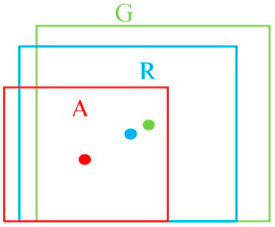
Figure 7.
Position correction diagram.
5. YOLOv3 vs. Faster R-CNN
In this study, the advantages and disadvantages of the object detection network based on YOLOv3 and Faster R-CNN are discussed. The test images were used to calculate their accuracy and compare other differences.
5.1. Comparison of Accuracy
In this study, the accuracy in the confusion matrix was used as the judgment index to compare the classification accuracy of the test images by models with different algorithms, as shown in Table 2 and Equation (20). To accommodate the presence of multiple defects in a single image, the accuracy analysis was designed to consider the overall performance of the defect detection system across all defect categories. The metrics used for evaluation, such as True Positives (TPs), False Positives (FPs), False Negatives (FNs), and True Negatives (TNs), were calculated collectively for all defect types. The confusion matrix, which forms the basis of our accuracy analysis, accounts for the system’s ability to correctly identify True Positives (correctly detected defects), False Positives (incorrectly identified defects), False Negatives (missed defects), and True Negatives (correctly identified absence of defects) across all defect categories present in the dataset.
Table 2.
Confusion matrix.
In this study, the existence of defects in the images was taken as the criterion to evaluate the defect detection system. A total of 765 datasets were used, and 55% of dataset images were defective. In total, 612 images of datasets were dedicated to the training phase and 153 datasets for testing. To ensure a fair and robust training process, we maintained a balanced representation of defective and non-defective PCB images. Specifically, 50% of the images in our training dataset contained defective PCB images, while the remaining 50% were non-defective PCB images. Considering this assumption, 111 defective and 42 non-defective images remained for testing data. This careful balancing of the training data aimed to enhance the model’s ability to generalize across various scenarios, promoting robustness in defect detection. Subsequently, during the testing phase, the dataset of 153 images comprised 72% with defects and 28% without defects. The test results are shown in Table 3.
Table 3.
Test result confusion matrix.
The results showed that the accuracy of the YOLOv3 algorithm and the Faster R-CNN algorithm was 95.4% and 83.7%, respectively, indicating that the YOLOv3 algorithm was better than the Faster R-CNN algorithm.
The precision, recall, and F1 score metrics provide a comprehensive evaluation of the performance of object detection models, YOLOv3 and Faster R-CNN, based on the given confusion matrices. The formulas for calculating precision, recall, and F1 are presented in Equations (21)–(23), respectively. These metrics provide a more nuanced understanding of the performance of each algorithm, proceeding beyond accuracy alone.
In this order, for YOLOv3, is the following:
Using the same scenario, Faster R-CNN is the following:
For YOLOv3, the high precision of approximately 95.6% indicates that when it predicts an object as defective, it is correct about 95.6% of the time. The recall of 98.2% signifies that YOLOv3 effectively identifies a significant portion of the actual defective items. The corresponding F1 score of 96.9% balances precision and recall, offering a robust measure of overall performance. On the other hand, Faster R-CNN demonstrates a precision of 83.1%, denoting that it correctly identifies defective items around 83.1% of the time. The recall of 97.3% indicates its ability to capture a substantial proportion of actual defective items. The F1 score for Faster R-CNN, at 89.6%, reflects a harmonious blend of precision and recall, portraying its overall effectiveness in object detection. These metrics collectively provide valuable insights into the strengths and weaknesses of each model, assisting in informed decision-making regarding their deployment in practical applications.
In the subsequent analysis, we assessed the efficacy of the Yolov3 model and evaluated its susceptibility to overfitting. The examination of overfitting during the optimization procedure necessitates scrutiny of the accuracy pertaining to the training data. To facilitate this evaluation, we incorporated a chart, as shown in Figure 8. In this figure, each epoch includes 100 iterations. The discernible trend from the chart illustrates a notable increase in accuracy throughout the training of the Yolov3 network. Beyond epoch 400, accuracy reaches a plateau, stabilizing at approximately 95%. This observation underscores the model’s capacity to maintain a consistent accuracy level after the specified epoch, suggesting a potential mitigation of overfitting effects.
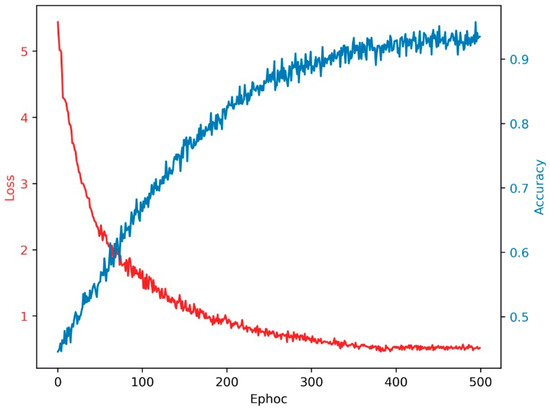
Figure 8.
Data training validation.
5.2. Comparison of Efficiency
In this study, the efficiency of the YOLOv3 and Faster R-CNN algorithms were further compared, as shown in Table 4, and illustrated as follows:
Table 4.
Efficiency comparison between YOLOv3 and Faster R-CNN.
- (1)
- Marking method: LabelImg Master software is used by both algorithms to mark, select, and classify the defect range on each image.
- (2)
- Operation mode: YOLOv3 and Faster R-CNN use input instructions to perform training and testing, but YOLOv3 is simpler than R-CNN. YOLOv3 requires only one file for parameter modification, while Faster R-CNN requires three files for modification. Regarding detection, YOLOv3 can detect multiple images at a time and automatically store images of the detection results. In contrast, Faster R-CNN can only detect one image at a time and cannot automatically store images of the detection results.
- (3)
- Training time: Based on the characteristics of the gold finger flaws discussed in this study, YOLOv3 took about two days to complete the training, while Faster R-CNN took about four days.
- (4)
- Learning mode: YOLOv3 and Faster R-CNN are used to build models, and both require classification of the training images before training, so they both belong to the supervised learning mode.
- (5)
- Deep learning architecture: Deep learning architecture mainly affects the speed of model training. From the perspective of training time, the speed of a one-stage architecture is faster than that of a two-stage architecture.
5.3. Defect Detection System Setup
As the accuracy of YOLOv3 at 95% was better than that of Faster R-CNN at 84%, YOLOv3 was selected to build the defect detection system. In this study, the determination to present a 95% accuracy was informed by multiple considerations, recognizing the potential for further refinement through methods like hyperparameter tuning. The rationale behind this reported accuracy is multifaceted. Firstly, it acknowledges the influence of application-specific requirements, where the acceptability of accuracy is contingent upon the unique demands and limitations of the particular application. In the realm of industrial defect detection, attaining a 95% accuracy might be considered satisfactory, especially if it aligns with or surpasses the quality control standards of the specific industry, with the acceptable threshold influenced by factors such as defect criticality and associated cost implications. Additionally, the reported accuracy reflects a conscientious trade-off between accuracy and other performance metrics like speed or computational resources, considering the need for a balance between a high detection rate and efficiency in terms of processing time and computational resources. Furthermore, the presented accuracy serves as a foundational baseline performance, with the awareness that further optimization opportunities exist, particularly through techniques like hyperparameter tuning. The decision not to extensively explore these advanced techniques initially was driven by the intention to establish a fundamental understanding of the defect detection system’s capabilities before delving into more intricate optimization strategies. The inspection process before and after the introduction of the defect detection system is shown in Table 5. After the introduction of the defect detection system, although the average PCB inspection time increased from 1.5 min to 3 minutes, the IQC sampling inspection was changed to a full inspection because the defect detection system adopted automatic image acquisition. As the accuracy of the defect detection system met the inspection standards of the case company, the SMT full inspection station was canceled.
Table 5.
Inspection process before and after the introduction of the defect detection system.
6. Conclusions
In the electronics industry, due to increasing demands for capacity and quality, incoming quality control standards are becoming more and more stringent. Currently, the industry’s incoming quality control is mainly based on manual sampling, which is time-consuming and prone to misjudgment. In this study, an automated defect detection system was built, in which deep learning was applied to the training iteration process of the defect detection model for the gold finger on the PCB to establish the defect determination criteria efficiently and accurately. In this study, the object detection networks of the YOLOv3 and Faster-R-CNN algorithms were evaluated. The results showed that the defect classification detection model based on the YOLOv3 network architecture could identify the location of defects with 95% accuracy. Therefore, the IQC sampling inspection was changed to a full inspection, and the SMT full inspection station was canceled for the purpose of reducing the inspection workforce.
This study is limited by its exclusive focus on defects related to the gold finger on printed circuit boards (PCBs), potentially hindering its generalizability to diverse defect types and industrial contexts. Additionally, the research primarily explores the YOLOv3 algorithm, neglecting alternative models and architectures that could offer valuable insights. Future research can overcome these limitations by broadening the scope of defect detection to include a wider range of defect types and industrial applications. Evaluating diverse deep-learning architectures and algorithms can enhance our understanding and potentially improve model performance. Integrating real-world data into the training process is crucial for ensuring the model’s adaptability to various manufacturing environments.
Author Contributions
C.-Y.H.; methodology, software, conceptualization, and editing. P.-X.T.; conceptualization and software. All authors have read and agreed to the published version of the manuscript.
Funding
This research is supported by the National Science Council under grant number 112AO29B.
Data Availability Statement
All data are available in this paper.
Conflicts of Interest
Author Pei-Xuan Tsai was employed by the company Sinbon Electronics. The remaining authors declare that the research was conducted in the absence of any commercial or financial relationships that could be construed as a potential conflict of interest.
References
- Chen, Y.; Ding, Y.; Zhao, F.; Zhang, E.; Wu, Z.; Shao, L. Surface Defect Detection Methods for Industrial Products: A Review. Appl. Sci. 2021, 11, 7657. [Google Scholar] [CrossRef]
- Hanbay, K.; Talu, M.F.; Özgüven, Ö.F. Fabric defect detection systems and methods—A systematic literature review. Optik 2016, 127, 11960–11973. [Google Scholar] [CrossRef]
- Westphal, E.; Seitz, H. A machine learning method for defect detection and visualization in selective laser sintering based on convolutional neural networks. Addit. Manuf. 2021, 41, 101965. [Google Scholar] [CrossRef]
- Mcmurray, S.; Sodhro, A.H. A Study on ML-Based Software Defect Detection for Security Traceability in Smart Healthcare Applications. Sensors 2023, 23, 3470. [Google Scholar] [CrossRef] [PubMed]
- Tabernik, D.; Šela, S.; Skvarč, J.; Skočaj, D. Segmentation-based deep-learning approach for surface-defect detection. J. Intell. Manuf. 2020, 31, 759–776. [Google Scholar] [CrossRef]
- Sui, X.; Leng, Z.; Wang, S. Machine learning based detection of transportation infrastructure internal defects using ground penetrating radar: A state-of-the-art review. Intell. Transp. Infrastr. 2023, 2, liad004. [Google Scholar] [CrossRef]
- Jha, S.B.; Babiceanu, R.F. Deep CNN-based visual defect detection: Survey of current literature. Comput. Ind. 2023, 148, 103911. [Google Scholar] [CrossRef]
- Papageorgiou, K.; Theodosiou, T.; Rapti, A.; Papageorgiou, E.I.; Dimitriou, N.; Tzovaras, D.; Margetis, G. A systematic review on machine learning methods for root cause analysis towards zero-defect manufacturing. Front. Manuf. Technol. 2022, 2, 972712. [Google Scholar] [CrossRef]
- Bhattacharya, A.; Cloutier, S.G. End-to-end deep learning framework for printed circuit board manufacturing defect classification. Sci. Rep. 2022, 12, 12559. [Google Scholar] [CrossRef]
- Chen, P.; Xie, F. A Machine Learning Approach for Automated Detection of Critical PCB Flaws in Optical Sensing Systems. Photonics 2023, 10, 984. [Google Scholar] [CrossRef]
- Soomro, I.A.; Ahmad, A.; Raza, R.H. Printed circuit board identification using deep convolutional neural networks to facilitate recycling. Resour. Conserv. Recycl. 2022, 177, 105963. [Google Scholar] [CrossRef]
- Volkan, K.A.Y.A.; Akgül, İ. Detection of defects in printed circuit boards with machine learning and deep learning algorithms. Avrupa Bilim Teknol. Dergisi 2022, 41, 183–186. [Google Scholar]
- Huang, C.-Y.; Lin, I.-C.; Liu, Y.-L. Applying Deep Learning to Construct a Defect Detection System for Ceramic Substrates. Appl. Sci. 2022, 12, 2269. [Google Scholar] [CrossRef]
- Huang, C.Y.; Ruano, M.; Chen, C.H.; Greene, C. Applying data mining methodology to establish an intelligent decision system for PCBA process. Solder. Surf. Mount Technol. 2019, 31, 271–278. [Google Scholar] [CrossRef]
- Huang, C.Y.; Hong, J.H.; Huang, E. Developing a machine vision inspection system for electronics failure analysis. IEEE Trans. Compon. Packag. Manuf. Technol. 2019, 9, 1912–1925. [Google Scholar] [CrossRef]
- Ray, S.; Mukherjee, J. A hybrid approach for detection and classification of the defects on printed circuit board. Int. J. Comput. Appl. 2015, 121, 42–48. [Google Scholar] [CrossRef]
- Li, Y.; Kuo, P.; Guo, J. Automatic Industry PCB Board DIP Process Defect Detection System Based on Deep Ensemble Self-Adaption Method. IEEE Trans. Compon. Packag. Manuf. Technol. 2021, 11, 312–323. [Google Scholar] [CrossRef]
- Çelik, A.; Küçükmanisa, A.; Sümer, A.; Çelebi, A.; Urhan, O. A real-time defective pixel detection system for LCDs using deep learning-based object detectors. J. Intell. Manuf. 2020, 33, 985–994. [Google Scholar] [CrossRef]
- Nepal, U.; Eslamiat, H. Comparing YOLOv3, YOLOv4 and YOLOv5 for Autonomous Landing Spot Detection in Faulty UAVs. Sensors 2022, 22, 464. [Google Scholar] [CrossRef]
- Ge, Z.; Liu, S.; Wang, F.; Li, Z.; Sun, J. Yolox: Exceeding yolo series in 2021. arXiv 2021, arXiv:2107.08430. [Google Scholar]
- Redmon, J.; Farhadi, A. Yolov3: An incremental improvement. arXiv 2018, arXiv:1804.02767. [Google Scholar]
- Redmon, J.; Farhadi, A. YOLO9000: Better, faster, stronger. In Proceedings of the IEEE Conference on Computer Vision and Pattern Recognition 2017, Honolulu, HI, USA, 21–26 July 2017; pp. 7263–7271. [Google Scholar]
- Girshick, R.; Donahue, J.; Darrell, T.; Malik, J. Rich feature hierarchies for accurate object detection and semantic segmentation. In Proceedings of the IEEE Conference on Computer Vision and Pattern Recognition 2014, Columbus, OH, USA, 23–28 June 2014; pp. 580–587. [Google Scholar]
Disclaimer/Publisher’s Note: The statements, opinions and data contained in all publications are solely those of the individual author(s) and contributor(s) and not of MDPI and/or the editor(s). MDPI and/or the editor(s) disclaim responsibility for any injury to people or property resulting from any ideas, methods, instructions or products referred to in the content. |
© 2024 by the authors. Licensee MDPI, Basel, Switzerland. This article is an open access article distributed under the terms and conditions of the Creative Commons Attribution (CC BY) license (https://creativecommons.org/licenses/by/4.0/).