Bad Data Repair for New Energy Stations in Power System Based on Multi-Model Parallel Integration Approach

Abstract

The accurate and reliable acquisition of measurement information is very important for the stable operation of power systems, especially the operation status information of new energy stations. With the increasing proportion of new energy stations in power systems, the quality issues of data from these stations, caused by communication congestion, interference, and network attacks, become more pronounced. In this paper, to deal with the issue of low accuracy and poor performance of bad data restoration in new energy stations, a novel deep learning approach by combining the modified long short-term memory (LSTM) neural network and Wasserstein generative adversarial network with gradient penalty (WGAN-GP) is proposed. The proposed method can be implemented in a parallel ensemble way. First, the normal data set acquired from multiple sections of new energy stations is utilized to train the modified LSTM and WGAN-GP model. Secondly, according to the data characteristics and rules captured by each model, the two models are systematically integrated and the bad data repair model pool is constructed. Subsequently, the results of model repair are screened and merged twice by the parallel integration framework to obtain the final repair result. Finally, the extensive experiments are carried out to verify the proposed method. The simulative results of energy stations in a real provincial power grid demonstrate that the proposed method can effectively repair bad data, thereby enhancing the data quality of new energy stations.

1. Introduction

In recent years, with the ongoing development of new energy systems, the integration of numerous new energy stations has led to a surge in the amount of data processed by power systems, making the data structures more complex [1]. In modern power systems, the tight integration of the physical and information layers has deepened the reliance of control centers on real-time measurement data. However, in addition to inevitable data noise, these real-time measurements frequently contain bad data. Such data not only distorts the system’s true state and adversely affects the accuracy and convergence of state estimation, but also poses significant challenges to the performance of subsequent advanced applications [2,3]. For instance, voltage amplitude errors in line parameter identification can be amplified a thousandfold in resistance identification [4]. In addition, network and time synchronization attacks on synchronous phasor data pose a threat to the safe and stable operation of power systems, sometimes even triggering cascading failures [5,6]. To deal with issues, repairing the bad measurement data of the new energy stations in real time is not only crucial for improving data quality and reliability, but also enhances the situational awareness capabilities of power systems, supporting their safe and stable operation.

Generally speaking, the methods for repairing bad data at new energy stations fall into two main categories: model-dependent repair methods and data-driven repair methods. Model-dependent repair methods require knowledge of the system’s topology and detailed parameters, which repairs the bad data through state estimation models. Reference [7] proposed a synchronous phasor data conditioning algorithm in which Kalman filtering and smoothing techniques for synchronous phasor data conditioning preprocessed the data before they reached the linear estimator to ensure the quality of the data obtained from phasor measurement units (PMUs), achieving the accurate restoration of PMU data. Reference [8] proposed a state estimator (PSE) method based on phasor measurement, which used an augmented state vector approach to identify and correct angle deviations and current scaling errors in phasor data, thereby improving data consistency and facilitating the repair of PMU data.

Although the aforementioned model-based methods for repairing bad data can effectively address anomalies, it is important to note their high dependency on models, requiring detailed system topology and parameter information. However, acquiring the accurate topology and detailed parameters of actual power systems is often challenging. In contrast, data-driven strategies for bad data repair can establish mappings between normal data sets and target data by directly learning intrinsic data relationships using data mining and machine learning methods, thereby accomplishing data repair. Consequently, data-driven repair methods have gained widespread attention in recent years [9,10,11,12]. Reference [13] proposed a data repair model, which is constructed with a generative adversarial network (GAN), which combines a temporal convolutional network (TCN) and a bi-directional long short-term memory network (BiLSTM) to repair the AIS data. Reference [14] proposed a bidirectional recurrent imputation time series (BRITS) method, leveraging bi-directional recurrent neural networks to capture the dynamic properties of time series data from both directions and provide accurate predictions for missing values. Reference [15] proposed a method using artificial neural networks to estimate missing synchrophasor data, predicting missing data values from existing complete data sets. Reference [16] proposed a method using an improved generative adversarial network, which can learn the distribution of measurement data in the power system and realize the reconstruction of missing measurement data with higher accuracy.

Data-driven repair methods, not reliant on detailed system models, offer significant flexibility. For the above-mentioned data-driven methods, they mostly rely on a single model. However, this dependence on a single training method significantly reduces the model’s generalization ability. Recently, ensemble learning has become a popular machine learning paradigm. Its core idea is to introduce diversity into models and appropriate combination strategies to overcome the limitations of single models, thereby enhancing overall repair accuracy [17]. Reference [18] proposed a multi-scale ensemble neural network method that utilizes long short-term memory (LSTM), gated recurrent units (GRU), and temporal convolutional networks (TCN) as the basic models. These networks are assembled on both single-model and multi-model scales to improve prediction accuracy. In dealing with large, variable, and nonlinear data sets, the heterogeneous base learning model can comprehensively capture the potential properties and associations of data with different distribution characteristics, and improve the overall performance of the model.

Therefore, addressing the issues of poor generalization and overfitting in single models, and considering the nonlinear time-series characteristics of new energy station data, in order to realize the reliable repair of abnormal data of new energy stations, a deep learning method combining modified LSTM with WGAN-GP is proposed in this paper. This method employs a parallel ensemble learning framework that integrates both modified LSTM and WGAN-GP models. Initially, the modified LSTM model is used to capture the temporal correlation features in the data of new energy stations, ensuring accurate fitting and prediction of time trends and patterns in the data. Simultaneously, the WGAN-GP model learns the distribution characteristics of the new energy station data, generating data similar to the actual data distribution, thereby enhancing robustness in real-world applications. Afterwards, by parallelly integrating the modified LSTM and WGAN-GP models, the strengths of both models are deeply fused to enhance the model’s generalization capabilities. Finally, simulation tests on the actual operational dataset of a new provincial energy station demonstrate that, compared to single data models, the proposed multi-model parallel ensemble method exhibits stronger generalization abilities. It can achieve the high-precision repair of bad data under various conditions, thus improving the data quality level of new energy stations.

The rest of the paper is organized as follows. Section 2 introduces the two selected models, the modified LSTM and the WGAN-GP. Section 3 is dedicated to presenting the multi-model parallel ensemble model. Section 4 provides a detailed discussion of the simulation results. Finally, Section 5 concludes by summarizing the article and discussing the future scope for the proposed method.

2. Multi-Model Parallel Integrated Data Repair Method

In this section, a novel approach by combining the modified long short-term memory (LSTM) neural network and Wasserstein generative adversarial network with gradient penalty (WGAN-GP) is developed and will be introduced in detail.

2.1. Modified LSTM Algorithm

2.1.1. Traditional LSTM Algorithm

Long short-term memory is a special type of recurrent neural network (RNN) first proposed in [19], primarily designed to deal with the issues of gradient disappearance and gradient explosion during long sequence training. Different from a traditional RNN, LSTM introduces three gate mechanisms: the forget gate, the input gate, and the output gate, along with a cell state. These gate mechanisms, implemented through neural networks, enable effective memory retention and selective forgetting of information within measurement data, thereby capturing temporal dependencies among the measured data.

In general, LSTM can be represented in the following form:

$$\left\{\begin{array}{l}{f}_t=\sigma (w_f[x_t,h_{t-1}]+b_f)\\ i_t=\sigma (w_i[x_t,h_{t-1}]+b_i)\\ o_t=\sigma (w_o[x_t,h_{t-1}]+b_o)\\ c_t=(f_t\otimes c_{t-1})\oplus (i_t\otimes \tanh (w_c[x_t,h_{t-1}]+b_c))\\ h_t=o_t\otimes \tanh (c_t)\end{array}\right.$$

(1)

where $f_t$ is the forgetting door; $i_t$ indicates an input gate; $o_t$ denotes an output gate; $c_t$ represents a cell state; $h_t$ is hidden state; $x_t$ is the input vector at time $t$; $t$ is a time step; $b_f$, $b_i$, $b_o$, $b_c$ are the deviation of the corresponding gate control unit; $w_f$, $w_i$, $w_o$, $w_c$ are the weight vector of the forget gate $f_t$, input gate $i_t$, output gate $o_t$, and the cell state $c_t$, respectively; $\sigma (·)$ and $\tanh (·)$ are the Sigmoid activation function and hyperbolic tangent function, respectively; $\otimes$ is the matrix multiplication operation; $\oplus$ is the matrix addition operation.

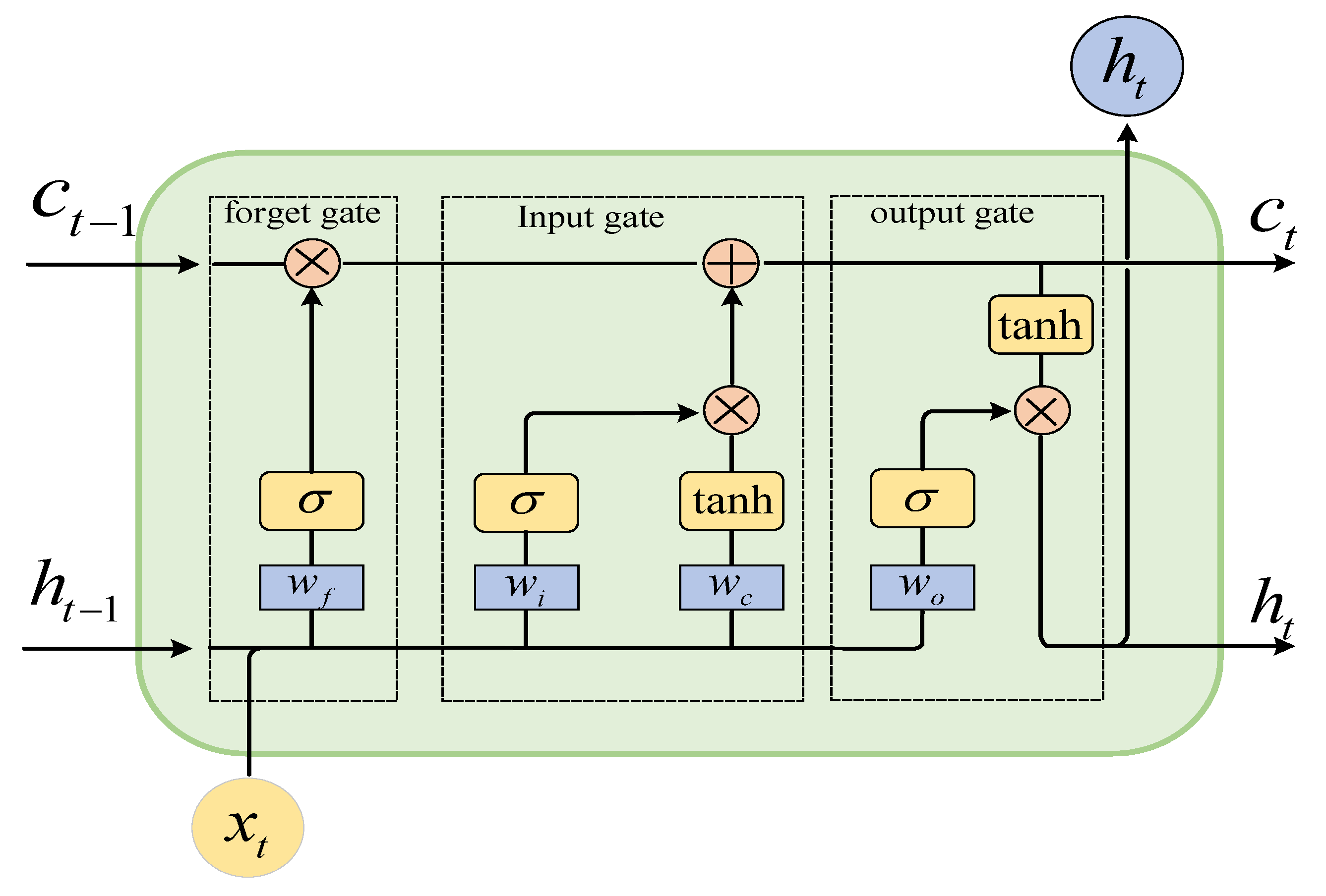
As shown in Figure 1, LSTM consists of input gates, control gates, forget gates, and output gates. Among these, the forget gate is responsible for filtering and discarding non-critical information from the cell state, allowing LSTM to disregard irrelevant information and retain valuable information for subsequent computations. The input gate regulates the input of new data information, enabling LSTM to update its internal cell state when processing new data. The output gate is in charge of transmitting information from the cell state to the next layer or the next time step, enabling LSTM to selectively output information that is useful for the current task. The cell state is the core of LSTM, spanning the entire time sequence and carrying essential information. The cell state can be updated through a combination of operations involving the forget gate and the input gate, ensuring the transmission of information in long sequences [19,20].

Despite its widespread application and robustness in handling sequential data, the traditional long short-term memory (LSTM) model is not without its limitations. One of the primary challenges associated with LSTM is its susceptibility to overfitting, especially in scenarios involving complex data sets with numerous parameters. Additionally, LSTM often faces difficulties in efficiently processing longer sequences, leading to a degradation in performance due to the vanishing gradient problem. In response to these shortcomings, our research focuses on further enhancements to the LSTM architecture. These improvements aim to address these specific limitations by optimizing the model’s architecture and training process. The following sections detail the methodologies employed to refine the LSTM model, encompassing optimization algorithms and regularization techniques.

2.1.2. Adam Optimization Algorithm

Adam optimization algorithm is a learning rate adaptive optimization algorithm [21]. Adam algorithm can be understood as a learning rate adaptive optimizer with momentum method. It is an extension of stochastic gradient descent and can replace the classical stochastic gradient descent method to update network weights more effectively. It estimates the gradient first and second moments of each parameter according to the objective function, calculated using the exponential moving average. In order to solve the problem of high noise and gradient dilution during parameter space iteration, the feature scaling of the gradient of each parameter is kept constant. The formula is derived as follows:

$$\left\{\begin{array}{c}{\theta }_i^{(k+1)}={\theta }_i^{(k)}-g_i^{(k)}\\ g_i^{(k)}=\frac{\eta {\widehat{v}}_i^{(k)}}{\sqrt{{\widehat{s}}_i^{(k)}+\epsilon }}\hfill \end{array}\right.$$

(2)

$$\left\{\begin{array}{c}{\widehat{v}}_i^{(k)}=\frac{v_i^{(k)}}{1-{\beta }_1^k}\\ {\widehat{s}}_i^{(k)}=\frac{s_i^{(k)}}{1-{\beta }_2^k}\end{array}\right.$$

(3)

where $k$ is the number of iterations; ${\theta }_i^{(k)}$ represents the $i$th characteristic parameter in the iterative process; $g_i^{(k)}$ denotes the descending distance value along the gradient direction; $s_i^{(k)}$ indicates the exponential decay average of the historical gradient; $v_i^{(k)}$ is the exponential decay average of the quadratic historical gradient; ${\widehat{s}}_i^{(k)}$ and ${\widehat{v}}_i^{(k)}$ are the deviation correction values of $s_i^{(k)}$ and $v_i^{(k)}$, respectively. Hyperparameter $\eta$ = 0.001; $\epsilon$ is manually entered parameters; Hyperparameter ${\beta }_1$ = 0.9; ${\beta }_2$ = 0.999.

Adam optimization algorithm in LSTM has significant advantages over the traditional stochastic gradient descent (SGD). With Adam, the learning rate can be adjusted more easily, helping to overcome the problem of disappearing or exploding gradients. The adaptive performance of Adam makes it more suitable to deal with different gradient characteristics of different parameters, thus, improving the training efficiency and convergence speed.

2.1.3. Dropout Regularization

Dropout regularization is a technique commonly used in neural network training to prevent models from overfitting [22]. The core idea of dropout is to randomly turn off a subset of neurons in the network during each training iteration, which can reduce the complex co-adaptive relationships between neurons. 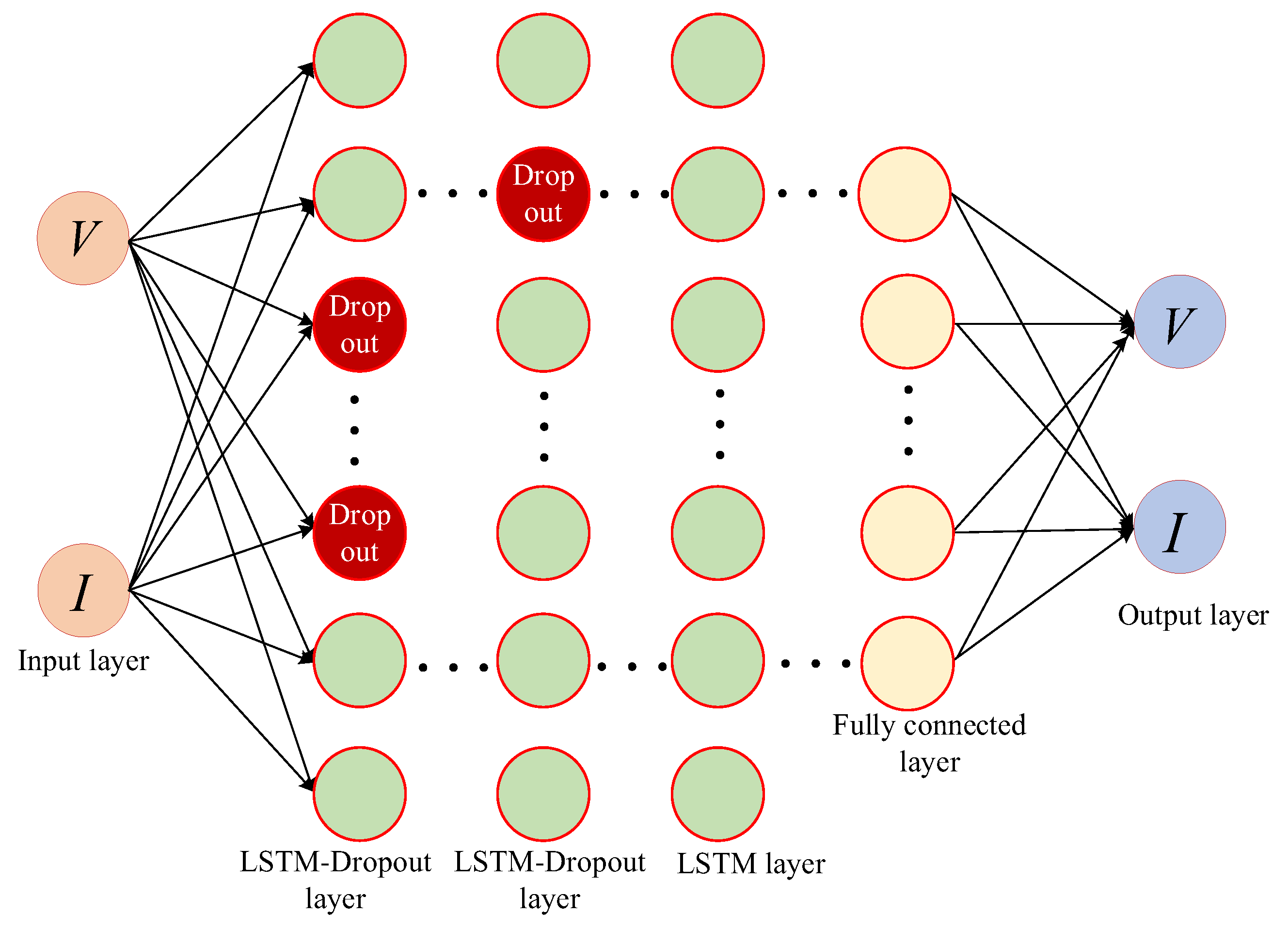Dropout regularization is introduced into the structure of the long short-term memory network (LSTM) [23] to enhance the generalization ability of the model. While LSTMs are more effective than traditional RNN at capturing long-term dependencies, they still run the risk of overfitting. By adding dropout regularization to the LSTM structure, a subset of connections or neurons in the network can be randomly dropped during training. This method can reduce the complex co-adaptive relationship between LSTM units and reduce the overfitting of the training data. Slightly different from standard dropout, when dropout is applied in LSTM, it is usually applied with different dropout proportions in different parts of the LSTM unit (such as input gate, forget gate, output gate) or between different layers to avoid excessive impact on the time dependence of LSTM. The modified LSTM model with dropout is shown in Figure 2.

2.2. WGAN-GP Algorithm

Generative adversarial network (GAN) is a type of deep learning model [24]. This model is capable of generating data with similar characteristics to the training data. GAN consists of two opposing networks: a generator and a discriminator. The generator’s task is to produce data samples resembling the distribution of real data, while the discriminator’s task is to distinguish between generated data and real data. These two networks learn from each other in an adversarial environment. The generator continuously improves its ability to generate realistic data, while the discriminator aims to enhance its capability to distinguish between real and generated data. As the training progresses, the generator eventually becomes proficient at creating samples that exhibit characteristics similar to the real data.

The objective function of the original generated adversarial network is as follows:

$$\begin{array}{ll}L(G,D)=& \underset{G}{\min } \underset{D}{\max }\{E_{x~p_r(x)}[\lg (D(x))]\\ & +E_{x~p_{g(z)}}[\lg (1-D(G(z))]\}\end{array}$$

(4)

where $L(·)$ is the objective function of generator and discriminator; $E(·)$ denotes the expectation function; $G(·)$ represents the generator functions; $D(·)$ is the discriminator function; $P_r(·)$ indicates the distribution of the objective function $x$; $P_g(·)$ is the noise data distribution; $z$ is the input noise data vector.

The traditional GAN model often exhibits a certain instability during training, which can lead to the problem of mode collapse. This issue refers to the generator’s tendency to produce highly similar samples, resulting in a lack of diversity in the generated samples [25]. In such cases, the generator struggles to capture the diversity present in the training data, thus failing to effectively generate new and diverse data samples. To address this problem, one approach is to introduce the Wasserstein distance to measure the discrepancy between generated data and real data. The definition of the Wasserstein distance is as follows:

$$W(P_r,P_g)=\frac{1}{K}\underset{‖f‖\le K}{\sup }(\underset{x~P_r(x)}{E}[f(x)]-\underset{\tilde{x}~P_g(\tilde{x})}{E}[f(\tilde{x})])$$

(5)

where $K$ represents the Lipschitz constant; $\sup (·)$ is the upper bound; $x$ is the raw data; $\tilde{x}$ is the generated data.

During the actual operation of WGAN, to ensure training stability, it is necessary to perform weight clipping on the discriminator. However, this weight clipping approach might lead to issues such as exploding gradients and non-convergence. To address this problem, based on the WGAN, a gradient penalty is introduced to regularize the gradients of the discriminator. The gradient penalty term helps ensure smoothness during the training process and encourages the generator to produce more diverse and higher-quality samples. The loss function of the WGAN-GP model can be represented as follows:

$$\begin{array}{ll}L(G,D)=& \underset{G}{\min } \underset{D}{\max }\{\underset{x~P_r(x)}{E}[D(x)]-\underset{z~P_g(z)}{E}[D(G(z))]\\ & +\lambda \underset{\widehat{x}~P_{\widehat{x}}(\widehat{x})}{E}{[{‖\nabla \widehat{x}D(\widehat{x})‖}_p-1]}^2\end{array}$$

(6)

where $\lambda$ represents the gradient penalty coefficient; $\widehat{x}=\alpha x+(1-\alpha )G(z)$ indicates a random interpolation between the real data and the generated data; $\alpha$ is the number randomly sampled from the uniform distribution [0, 1]; $P_{\widehat{x}}(·)$ is an interpolation distribution formed between the real data distribution and the generated data distribution. ${‖·‖}_p$ is p norm; $\nabla$ is the gradient operator.

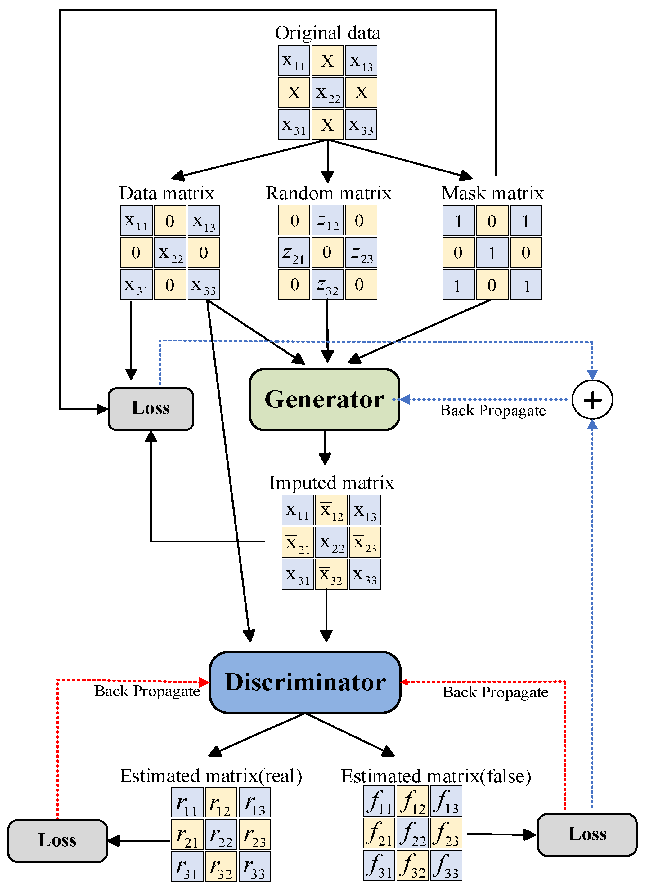
By enhancing the discriminator, WGAN-GP not only overcomes the issue of mode collapse but also improves the stability of training in GANs. This enhancement enables the generator to produce more diverse and higher-quality data samples. Figure 3 depicts the architecture of the WGAN-GP network.

2.3. WGAN-GP Algorithm

Ensemble learning is a machine learning method that leverages the combination of multiple simple models to obtain a composite model with improved performance, thereby enhancing the accuracy and generalization capabilities of the model [26]. The primary strategies of ensemble learning involve generating diversity, model training, and model combination. Common ensemble learning techniques include bagging, boosting, and stacking. Ensemble learning not only enhances model performance but also allows researchers to design combination approaches tailored to specific machine learning problems to obtain more robust solutions.

As an extension of ensemble learning, parallel ensemble learning can enhance the efficiency of ensemble learning through parallel computing [27]. In the conventional ensemble learning, the training and prediction of each base model are executed sequentially. However, in the parallel ensemble learning, multiple base models can be trained and make predictions simultaneously on different computing resources. Parallel ensemble learning can significantly reduce the time required for model training and prediction, thereby enhancing the model’s performance. This is particularly significant for handling large-scale data sets and achieving real-time predictions.

This paper adopts the bootstrap aggregating (Bagging) algorithm from parallel ensemble learning to integrate LSTM and WGAN-GP. Bagging is a commonly used basic strategy in ensemble learning [28], and its fundamental principle is depicted in Figure 4. The core idea of the Bagging algorithm involves multiple rounds of resampling the original dataset to generate several diverse training subsets. These subsets are then used to train multiple models. Finally, the predictions of these models are integrated through voting or averaging to produce the ultimate prediction.

Generally, for the regression problem, Bagging’s aggregated results often employ either the averaging method or the weighted averaging method to combine the predictions from all base models. Specifically, the averaging method accumulates the predictions of each base model and then divides the sum by the number of base learners to obtain the final prediction value. On the other hand, the weighted averaging method assigns different weights to each base model based on its performance. Then, it calculates the weighted average as the final prediction result [29].

To ensure the quality of the repair while considering the differences and effectiveness of each base learning model, based on the theory of minimizing loss [30], this paper proposes a multi-model prediction result fusion strategy based on an improved weighted averaging method. This method allows multiple models to contribute predictions proportionally based on their trustworthiness or estimated performance, thereby enhancing the performance and stability of the ensemble model and minimizing prediction errors. By analyzing the loss value of each model, weights can be assigned to each model and integrated with the predictions of the base models, ensuring the accuracy of data repair.

Therefore, the weight calculation formulas for the predictions from the modified LSTM algorithm and the WGAN-GP algorithm are as follows:

$$\alpha =\frac{loss\_wgan}{loss\_lstm+loss\_wgan}$$

(7)

$$\beta =\frac{loss\_lstm}{loss\_lstm+loss\_wgan}$$

(8)

$$Y_{pre}={\omega }_1{Y}_{pre\_lstm}+{\omega }_2{Y}_{pre\_wgan}$$

(9)

where ${\omega }_1$ denotes the weight of the predicted value of modified LSTM model; ${\omega }_2$ represents the weight of the predicted value of WGAN-GP model; $loss\_lstm$ indicates the loss function value of the modified LSTM training model; $loss\_wgan$ is the loss function value of the WGAN-GP training model; $Y_{pre}$ is the result value of multi-model fusion prediction; $Y_{pre\_lstm}$ is the predicted value of the modified LSTM model; $Y_{pre\_wgan}$ is the predicted value of the WGAN-GP model.

3. Bad Data Repair Method for New Energy Station Based on Multi-Model Parallel Ensemble

In order to overcome the potential issues such as overfitting associated with existing single models, in this paper, by combining the modified LSTM model and WGAN-GP model, a novel multi-model parallel ensemble method for the repair of bad data of new energy stations is developed. The proposed method can merge the strengths of multiple models to enhance the repairing performance and robustness. By training multiple models in parallel on different data or feature subsets, it can effectively reduce training time and increase the diversity of models, thereby reducing the risk of overfitting and having better model interpretability.

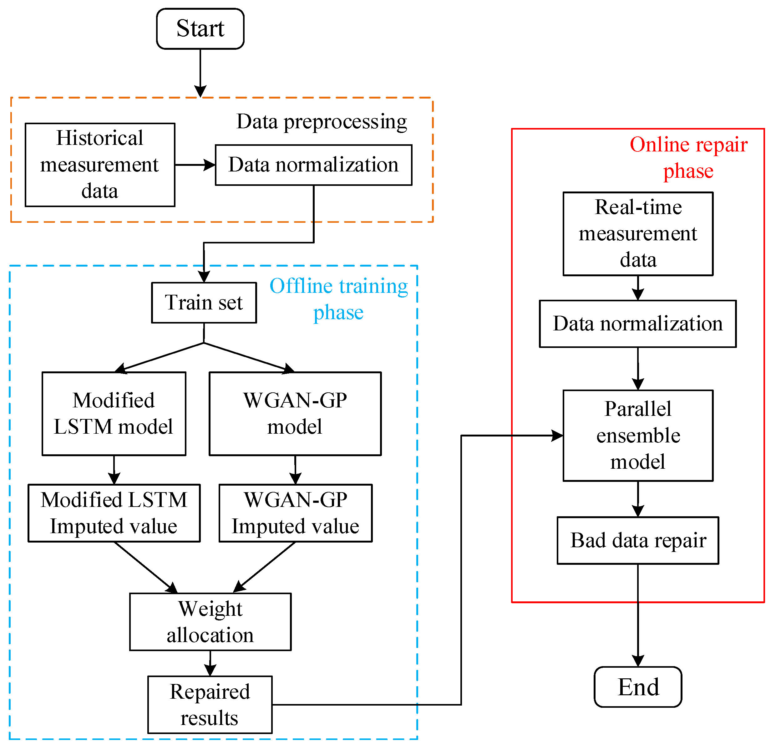
Specifically, the application of a multi-model parallel ensemble data repair method for the correction process of adverse data in new energy station is illustrated in Figure 5. It mainly consists of two stages: (1) offline training; (2) online repair.

(1)

Offline Training

The offline training stage is the key step in building the integrated model, which involves the training and weight determination of the model.

Step 1: Model training. First, the current and voltage historical data of the new energy station are normalized and divided into a training set and a test set, in which the ratio of training set and test set is usually 4:1. Then, self-sampling is utilized to randomly extract multiple subsets from the training data, each containing 70% of the original training data set. Finally, the improved LSTM and WGAN-GP models are trained with each data subset to determine their respective model parameters and structures.

Step 2: Weight calculation. Since the improved LSTM and WGAN-GP each represent different repair strategies, it is necessary to clarify the weight allocation between them. First, loss measurement is used to evaluate the error between the model repair results and the real data, which provides a quantitative evaluation basis for the following steps. Then, the loss values of the improved LSTM and WGAN-GP models in the process of data repair are calculated individually to evaluate the repair efficiency of each model. A lower loss value indicates that the model has a better repair effect, while a higher loss value reflects that the model has a poor repair effect. Finally, the weights of the improved LSTM and WGAN-GP models are determined according to Formulas (7)–(9).

Step 3: Integrated model building. Following the completion of preliminary data preparation, training of individual models, and weight allocation, this stage employs the architecture of parallel ensemble learning. The previously trained, improved LSTM and WGAN-GP models are fused to create an efficient integrated learning model. Initially, the outputs of the two models are fed into a specifically designed fully connected layer, tasked with integrating the outputs of both models to generate a comprehensive repair result. Subsequently, within the fully connected layer, the outputs of the improved LSTM and WGAN-GP models are weighted and fused using the weight strategy determined in Step 2. Finally, for this parallel ensemble learning model, further training and optimization are conducted by adjusting the model’s parameters and structure to ensure its effectiveness in handling real-world data repair tasks.

(2)

Online Repair

The online stage is the practical application stage, which mainly repairs the real-time measurement data.

Step 1: Real measurement data input. At this stage, the three sets of measured current and voltage data of the new energy station are preprocessed to ensure that the data format is consistent with the model training. Then, the measured data after processing are input into the trained model.

Step 2: Repair bad data online. First, the model loads the parameters and structures learned during the offline training phase. Then, using the knowledge of offline training, the model can repair the actual measurement data.

In summary, establishing an effective bad data repair system for new energy stations requires two key phases: offline training and online repair. The offline phase focuses on training the repair models and determining the weights between different models to ensure the extraction of time-series data characteristics and the generation of high-quality data. The online phase then utilizes the previously trained models to repair bad data.

Remark 1.

In this paper, an innovative approach is developed for the bad data repair of new energy stations in power systems, leveraging a novel integration of modified LSTM and WGAN-GP models in a parallel framework. Compared with a single model, the resulting model significantly improves the robustness and generalization ability of the model, and the accuracy and efficiency of data repair are also significantly improved.

Figure 5. Bad data repair flow chart based on multi-model parallel ensemble learning.

Figure 5. Bad data repair flow chart based on multi-model parallel ensemble learning.

4. Case Analysis

In this paper, a PC configured with AMD Ryzen 7 5800 H 3.20 GHz CPU, 16 GB RAM and a Windows 10 64-bit operating system is used to compile Python programs with Pytorch as the deep learning framework and to build an improved LSTM model and WGAN-GP model. The performance of the proposed algorithm is verified by actual new energy station data.

4.1. Experimental Data Set

In practical applications, the true value of abnormal or corrupted data is often difficult to obtain. This means that the accuracy of data repair cannot be evaluated by directly comparing the true value, so data repair becomes a typical unsupervised learning problem [31]. To more intuitively assess and understand the effects of data repair, a strategy can be employed: simulate the generation of data sets containing bad data from a complete and reliable data set. Then, the proposed method is used to repair these bad data, and the repaired data are compared with the original real data, so as to evaluate the accuracy of the repair effect. In addition, because the data are often affected by random factors and uncertainties, it is difficult to predict the location and amount of bad data. In order to simulate this real scenario and ensure the quantity of bad data in each experiment, this study uses the mask matrix strategy to ensure the randomness and authenticity of the generated bad data, so as to be closer to the abnormal data situation in actual operation.

In order to verify the effectiveness of the proposed method, an actual wind farm in a province was selected as the research object, and the real-time current and voltage measurement data of three PMUs were randomly selected as the test set. Each group contained 200 data points, and the overall data dimension was 200 × 6. In order to ensure the generalization ability of the model, the complete data set is divided into the training set and the test set in a 4:1 ratio. In the test set, some measurement data in the data set are randomly added with mixed noise to simulate the bad data that may appear in the real scene. In general, various bad data conditions are characterized by increasing or decreasing the normal voltage and current measurement values by 5–10%.

Before training the model, it is necessary to preprocess the historical measurement data to ensure that different data levels or ranges will not adversely affect the training of the model and capture the real characteristics of the data. For data normalization, the calculation formula is as follows

$$x_{Nor}=\frac{x-\min (x)}{\max (x)-\min (x)}$$

(10)

where $x$ is the data that need to be normalized; $x_{Nor}$ is the normalized value; $\min (x)$ is the minimum value of the feature $x$; $\max (x)$ is the minimum value of the feature $x$.

4.2. Experiment and Result Analysis

4.2.1. Data Repair Evaluation Index

In order to quantitatively test the data repair effect of the proposed model, root-mean-square error (RMSE) and mean absolute percentage error (MAPE) were selected in this paper. MAPE is used as an evaluation index of the data repair effect [31]. Among them, RMSE can measure the deviation between the predicted value and the actual value, while MAPE gives the relative relationship between the predicted error and the actual value, which can more intuitively understand the accuracy of the repair effect.

The performance evaluation indexes are defined as follows:

$${\mu }_{RMSE}=\sqrt{\frac{1}{n}{\displaystyle \sum _{i=1}^n{(y_i^{real}-y_i^{pre})}^2}}$$

(11)

$${\mu }_{MAPE}=\frac{1}{n}{\displaystyle \sum _{i=1}^n\left|\frac{y_i^{real}-y_i^{pre}}{y_i^{real}}\right|}$$

(12)

where $n$ is the number of bad data; $y_i^{real}$ is the actual quantity measurement; $y_i^{pre}$ is the repair value.

4.2.2. Case Setting

In order to accurately evaluate the repair effect of the bad data of the proposed method, two comparative experimental scenarios were set up for verification based on the selected experimental data set.

Scenario 1.

Generate bad data randomly in the original data set, compare the data repair effect of LSTM and the proposed method, and evaluate the bad data repair performance of the proposed method.

Scenario 2.

Under the condition of different proportions of bad data, the method proposed in this paper is comprehensively compared with several unsupervised data repair methods.

4.3. Random Bad Data Situation

In order to intuitively demonstrate the superiority in repairing bad data of the parallel integration strategy proposed in this paper over a single model, the single model LSTM and the proposed model are selected in this scenario for comparative experiments. The experiment randomly generates 5% bad data on the original data set, and repaired bad data on the same data set, aiming to reveal the improvement and advantages of the proposed method compared with a single model in processing the same data.

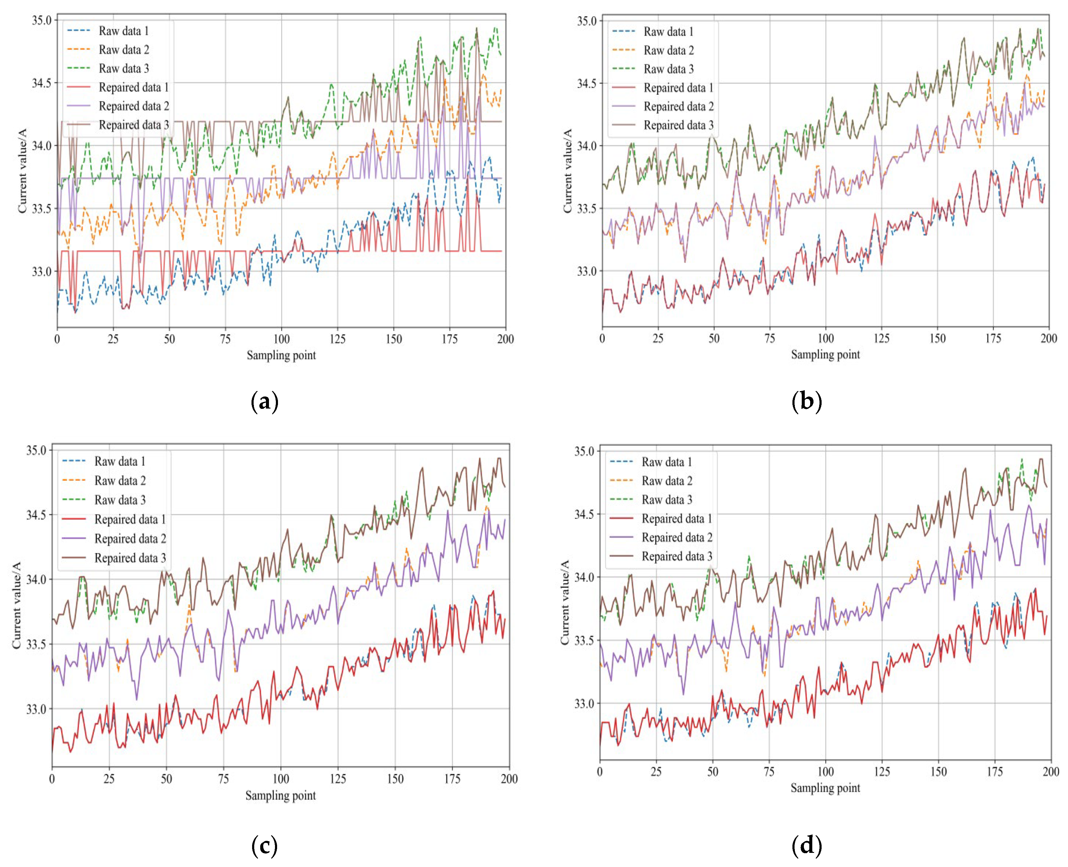
The LSTM method and the method proposed in this paper were used to repair the bad data. The test results are shown in Figure 6. As can be seen from the results shown in Figure 6, the LSTM method has a certain repair effect on a single item of bad data. However, in the face of continuous bad data, the LSTM method has a poor repair performance, and the output is continuous and unchanged data. This is because LSTM over-relies on historical data to make predictions in the face of continuous bad data, fails to effectively capture the characteristics of the current continuous bad data, and so overfitting occurs, resulting in continuous and identical data.

In addition, Figure 6 also shows the repair results of bad data using the method proposed in this paper. It can be seen that when the same continuous bad data are repaired using the proposed method in this paper, the repair result is an item of data with a similar distribution to the original data, and the overfitting phenomenon is effectively alleviated. These results show that the proposed method can better capture data features by integrating the prediction of multiple models, reducing the over-dependence on historical data, avoiding the overfitting problem of a single model, and realizing the high-precision repair of continuous bad data.

In order to evaluate the performance of the proposed method more comprehensively,

Table 1. Case system parameters setting.

Method	RMSE	MAPE
LSTM	0.1859	0.0440%
Proposed method	0.0548	0.0138%

gives the calculation results of the root-mean-square error and mean absolute percentage error of LSTM and the proposed method in this paper. It can be seen from the results in Table 1 that the error of the repair method proposed in this paper is smaller than that of the single LSTM model. This indicates that the proposed method is more accurate and effective in repairing bad data.

In summary, the method proposed in this paper significantly improves the repair quality of bad data by integrating multiple models. Compared with a single LSTM model, it can effectively alleviate the overfitting phenomenon and show higher accuracy and effect.

4.4. Different Proportions of Bad Data

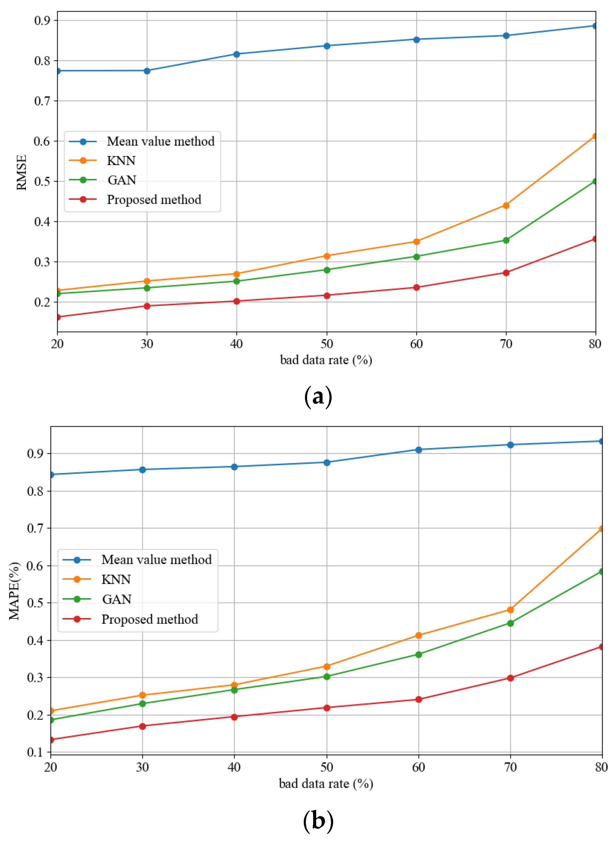
In order to further systematically and comprehensively verify the performance of the method proposed in this study, in this scenario, three unsupervised bad data repair methods are selected: mean value repair method, KNN repair method, and GAN repair method, and comparative tests are conducted. The experiment randomly generated eight different percentages of bad data on the original data set: 20%, 30%, 40%, 50%, 60%, 70%, and 80%. In each ratio of bad data, four repair methods were tested and compared in detail.

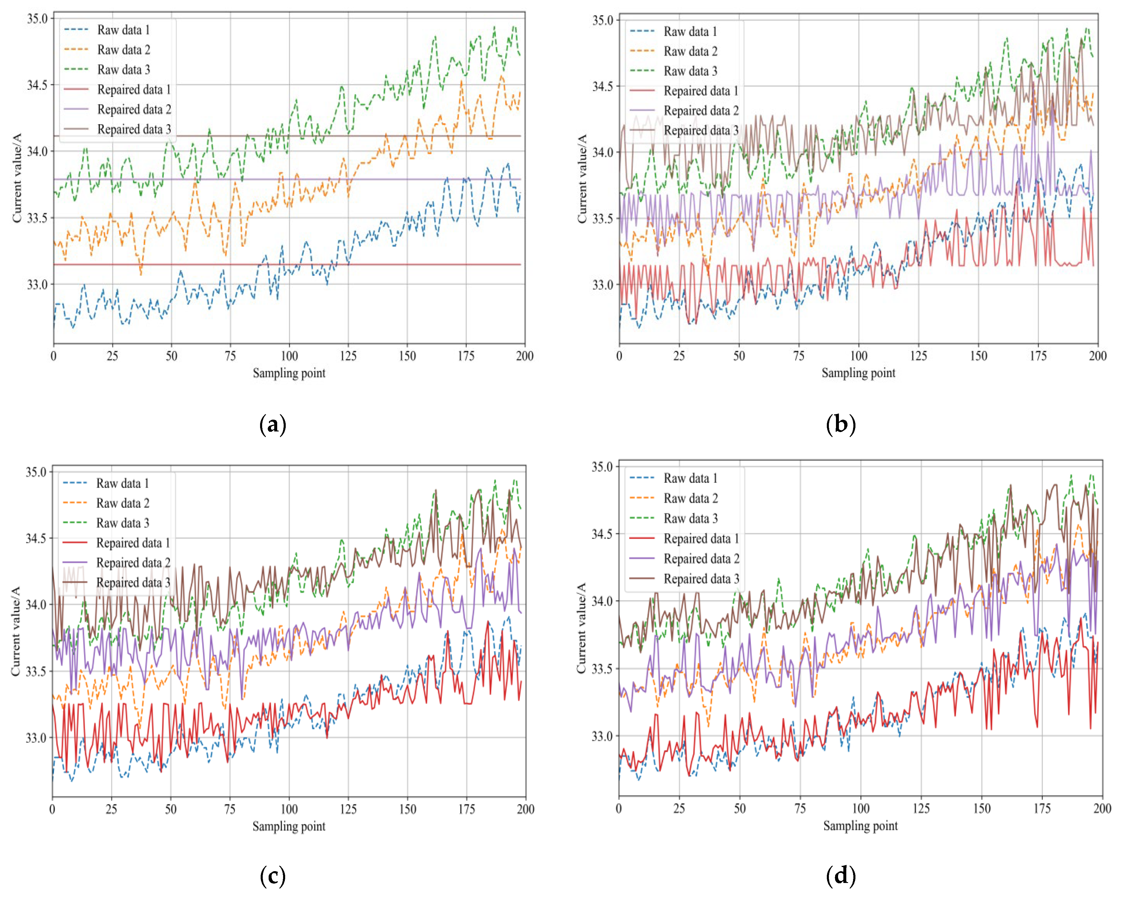
Due to the page limit, this article only displays a comparison of the repair effects of current values under 20% and 80% proportions of bad data. Figure 7 and Figure 8 show the repair results obtained by the mean value method, KNN method, GAN method, and the proposed method under the different proportions of bad data. Clearly, from these figures, it can be observed that under all proportion conditions, the repair effect of the mean value method is significantly inferior to the other three algorithms.

Under low proportions of bad data conditions, the repair effects of KNN, GAN, and the method proposed in this study are similar. However, with the increase in the proportion of bad data, the repair effects of KNN and GAN gradually deteriorate. In contrast, the method proposed in this paper still has an excellent repair effect. In order to more thoroughly compare the efficiency of these four algorithms in handling different proportions of bad data, this article also provides a comparative analysis of the root-mean-square error and mean absolute percentage error for these methods.

Figure 9 shows the root-mean-square and average percentage errors of each repair method with 20% to 80% bad data. It can be seen that the mean method consistently maintains high RMSE and MAPE values, which indicates that the method is less capable of repairing in the face of bad data. In contrast, the KNN repair method, GAN repair method, and method proposed in this paper can obtain smaller RMSE values and MAPE values when the proportion of bad data is small (<50%), and the error index of the proposed method is significantly smaller than that of other methods. However, in the case of a large proportion of bad data (>50%), as the proportion of bad data increases, the bad data repair effect of each model decreases; however, it can be seen that the performance of the proposed method is still far superior to other methods.

Specifically, from the comparison results of error indicators of each test method under different proportions of bad data in

Table 2. Root-mean-square error of each method under different proportions of bad data.

Loss Rate/%	RMSE
	Mean Value Method	LSTM	GAN	Proposed Method
20	0.7742	0.2283	0.2201	0.1621
30	0.7746	0.2516	0.2346	0.1897
40	0.8159	0.2698	0.2512	0.2017
50	0.8363	0.3143	0.2796	0.2162
60	0.8524	0.3496	0.3127	0.2355
70	0.8615	0.4403	0.3528	0.2724
80	0.8862	0.6124	0.5003	0.3564

and

Table 3. Mean absolute percentage error of each method with different proportions of bad data.

Loss Rate/%	MAPE (%)
	Mean Value Method	KNN	GAN	Proposed Method
20	0.8435	0.2098	0.1856	0.1325
30	0.8569	0.2517	0.2291	0.1693
40	0.8647	0.2796	0.2667	0.1943
50	0.8762	0.3295	0.3018	0.2184
60	0.9104	0.4121	0.3612	0.2402
70	0.9235	0.4812	0.4454	0.2979
80	0.9331	0.6987	0.5842	0.3801

, it can be seen that with a data missing rate of 20%, the data repair accuracy of the proposed method is improved by 36.57% compared with KNN and 28.61% compared with GAN. With a data missing rate of 50%, the proposed method improves the data repair accuracy by 33.71% compared with KNN and 27.63% compared with GAN. Even in the extreme case where the proportion of bad data is as high as 80%, the data repair accuracy of the method proposed in this paper still remains at a high level, with an MAPE of 0.3801%.

The above experimental results show that compared with the traditional mean repair method and KNN and GAN single model repair method, the multi-model integration-based bad data repair method proposed in this paper can obtain better bad data repair accuracy and has stronger generalization ability. This is because the proposed method can more comprehensively capture the different distribution characteristics of the new energy station measurement data and mine the potential characteristics and correlation of the data, so that it can better adapt to and deal with bad data, improve the overall performance of the model, and thus provide more accurate repair results under various bad data scenarios.

5. Conclusions

To deal with the issue of low accuracy and poor performance of bad data repair in new energy stations, this paper proposes a novel deep learning approach by combining modified LSTM and WGAN-GP models. Based on the experimental results, the following conclusions can be drawn.

(1) The adoption of the modified LSTM model has effectively mitigated the problems of gradient vanishing or explosion, which is a notable progression in neural network training. This modification can significantly reduce the model’s tendency to overfitting of training data, thereby improving both the efficiency of the training and the generalization ability of the model.

(2) This ensemble approach has not only facilitated effective feature extraction from normal measurement data, but has also significantly improved the overall performance of the system. By leveraging the strengths of both models, our approach can achieve a more nuanced and comprehensive analysis of the data, resulting in more accurate and reliable repair data results.

(3) The multi-model parallel ensemble method proposed in this paper has significant advantages over a single model, which can achieve the high-precision repair of bad data under various working conditions and has stronger generalization ability.

Since the approach proposed in this paper for repairing bad data from new energy field stations based on the parallel ensemble of multiple models shows superiority, the conclusions drawn from this study can guide more complex models and integration strategies. Therefore, further research should focus on how to optimize this parallel integration strategy. This may include adjusting the weight allocation between different models, exploring the integration effects of different types of neural network models such as convolutional neural networks (CNNs) or recurrent neural networks (RNNs), as well as improving the existing models to better handle specific types of bad data.

References

- Han, X.; Li, T.; Zhang, D.; Zhou, X. New issues and key technologies of new power system planning under double carbon goals. High Volt. Eng. 2021, 47, 3036–3046. [Google Scholar]
- Zhu, L.; Hill, D.J. Cost-effective bad synchrophasor data detection based on unsupervised time-series data analytic. IEEE Internet Things J. 2021, 8, 2027–2039. [Google Scholar] [CrossRef]
- Peng, Z.; Lu, Y.; Zhang, Y.; Deng, W.; Zeng, Q. The online frequency security assessment of a power system considering the time-varying characteristics of renewable energy inertia. Electronics 2023, 12, 2205. [Google Scholar] [CrossRef]
- Xue, A.; Xu, F.; Martin, K.E.; Xu, J.; You, H.; Bi, T. Linear approximations for the influence of phasor angle difference errors on line parameter calculation. IEEE Trans. Power Syst. 2019, 34, 3455–3464. [Google Scholar] [CrossRef]
- Jiang, X.; Zhang, J.; Harding, B.J.; Makela, J.J.; Domı, A.D. Spoofing GPS receiver clock offset of phasor measurement units. IEEE Trans. Power Syst. 2013, 28, 3253–3262. [Google Scholar] [CrossRef]
- Shepard, D.P.; Humphreys, T.E.; Fansler, A. Evaluation of the vulnerability of phasor measurement units to GPS spoofing attacks. Int. J. Crit. Infrastruct. Prot. 2012, 5, 146–153. [Google Scholar] [CrossRef]
- Jones, K.D.; Pal, A.; Thorp, J.S. Methodology for performing synchrophasor data conditioning and validation. IEEE Trans. Power Syst. 2015, 30, 1121–1130. [Google Scholar] [CrossRef]
- Ghiocel, S.G.; Chow, J.H.; Stefopoulos, G.; Fardanesh, B.; Maragal, D.; Blanchard, B.; Razanousky, M.; Bertagnolli, D.B. Phasor measurement based state estimation for synchronous phasor data quality improvement and power transfer interface monitoring. IEEE Trans. Power Syst. 2014, 29, 881–888. [Google Scholar] [CrossRef]
- Ma, M.; Qin, J.; Yang, D.; Zhou, B.; Pang, Y. A review of the application of artificial intelligence in power systems. J. Zhengzhou Univ. (Eng. Ed.) 2019, 40, 23–31. [Google Scholar]
- Xie, K.; Liu, J.; Liu, Y. A power system timing data recovery method based on improved VMD and attention mechanism Bi-directional CNN-GRU. Electronics 2023, 12, 1590. [Google Scholar] [CrossRef]
- Lattner, S.; Nistal, J. Stochastic restoration of heavily compressed musical audio using generative adversarial networks. Electronics 2021, 10, 1349. [Google Scholar] [CrossRef]
- Ma, J.; Cheng, J.C.P.; Jiang, F.; Chen, W.; Wang, M.; Zhai, C. A bi-directional missing data imputation scheme based on LSTM and transfer learning for building energy data. Energy Build. 2020, 216, 109941. [Google Scholar] [CrossRef]
- Zhang, W.; Jiang, W.; Liu, Q.; Wang, W. AIS data repair model based on generative adversarial network. Reliab. Eng. Syst. Saf. 2023, 240, 109572. [Google Scholar] [CrossRef]
- Lee, G.; Kwon, G.Y.; Kim, S.H.; Kim, D.I.; Kim, Y.; Nam, S.; Ko, B.; Kang, S.; Shin, Y.J. Missing entry estimation of synchrophasor data using artificial neural network. In Proceedings of the 9th International Conference on Power and Energy Systems (ICPES), Perth, WA, Australia, 10–12 December 2019; Institute of Electrical and Electronics Engineers Inc.: Perth, WA, Australia, 2019; pp. 1–6. [Google Scholar]
- Wang, S.; Chen, H.; Pan, Z.; Ling, T. A reconstruction method for missing data in power system measurement using an improved generative adversarial network. Proc. CSEE 2019, 39, 56–64. [Google Scholar]
- Wang, Y.; Zhang, Z.; Ma, J.; Jin, Q. KFRNN: An effective false data injection attack detection in smart grid based on Kalman filter and recurrent neural network. IEEE Internet Things J. 2022, 9, 6893–6904. [Google Scholar] [CrossRef]
- Hochreiterand, S.; Schmidhuber, J. Long short-term memory. Neural Comput. 1997, 9, 1735–1780. [Google Scholar] [CrossRef] [PubMed]
- Shen, Q.; Mo, L.; Liu, G.; Zhou, J.; Zhang, Y.; Ren, P. Short-term load forecasting based on multi-scale ensemble deep learning neural network. IEEE Access 2023, 11, 111963–111975. [Google Scholar] [CrossRef]
- Zhao, S.; Dong, X. Research on speech recognition based on improved LSTM deep neural network. J. Zhengzhou Univ. (Eng. Ed.) 2018, 39, 63–67. [Google Scholar]
- Kingma, D.P.; Ba, J.L. Adam: A method for stochastic optimization. In Proceedings of the International Conference on Learning Representations (ICLR), San Diego, CA, USA, 7–9 May 2015; pp. 1–15. [Google Scholar]
- Srivastava, N.; Hinton, G.; Krizhevsky, A.; Sutskever, I.; Salakhutdinov, R. Dropout: A simple way to prevent neural networks from overfitting. J. Mach. Learn. Res. 2014, 15, 1929–1958. [Google Scholar]
- Cui, H.; Li, F.; Tomsovic, K. Hybrid symbolic-numeric framework for power system modeling and analysis. IEEE Trans. Power Syst. 2021, 36, 1373–1384. [Google Scholar] [CrossRef]
- Goodfellow, I.; Pouget-Abadie, J.; Mirza, M.; Xu, B.; Warde-Farley, D.; Ozair, S.; Courville, A.; Bengio, Y. Generative adversarial nets. In Proceedings of Advances in Neural Information Processing Systems; MIT Press: Toronto, ON, Canada, 2014. [Google Scholar]
- Xu, M. Towards generalized implementation of wasserstein distance in GANs. In Proceedings of the AAAI Conference on Artificial Intelligence, Online, 2–9 February 2021; Volume 35, pp. 10514–10522. [Google Scholar]
- Dong, X.; Yu, Z.; Cao, W.; Shi, Y.; Ma, Q. A survey on ensemble learning. Front. Comput. Sci. 2020, 14, 241–258. [Google Scholar] [CrossRef]
- Woźniak, M.; Grana, M.; Corchado, E. A survey of multiple classifier systems as hybrid systems. Inf. Fusion 2014, 16, 3–17. [Google Scholar] [CrossRef]
- Odegua, R. An empirical study of ensemble techniques (bagging, boosting and stacking). In Proceedings of the Conference: Deep Learning IndabaXAt, Nigeria, Kenya, 25–31 August 2019. [Google Scholar]
- Xu, J.; Yang, Y. Ensemble learning method: Research review. J. Yunnan Univ. (Nat. Sci. Ed.) 2018, 40, 1082–1092. [Google Scholar]
- Ko, H.; Lee, J.; Byun, J.; Son, B.; Park, S. Loss-driven adversarial ensemble deep learning for online time series analysis. Sustainability 2019, 11, 3489. [Google Scholar] [CrossRef]
- Zhao, J.; Wang, J. Repairing adversarial samples based on SmsGAN. J. Zhengzhou Univ. (Eng. Ed.) 2021, 42, 50–55. [Google Scholar]
- Guo, X.; Li, Z.; Liu, H.; Bi, T. PMU loss data recovery method based on enhanced generative adversarial networks. Power Syst. Technol. 2022, 46, 2114–2121. [Google Scholar]