


Outdoor-to-Indoor mmWave Relaying with Massive MIMO: Impact of Imperfect Channel Estimation †

Communication Systems Department, INPT (Institut National des Postes et Télécommunications), Rabat 10100, Morocco
*
Author to whom correspondence should be addressed.
†
This paper is an extended version of our paper published in 6th International Conference on Advanced Communication Technologies and Networking (CommNet), Rabat, Morocco, 11–13 December 2023.
Electronics 2024, 13(10), 1857; https://doi.org/10.3390/electronics13101857
Submission received: 4 April 2024
/
Revised: 6 May 2024
/
Accepted: 8 May 2024
/
Published: 10 May 2024
(This article belongs to the Special Issue New Trends and Methods in Communication Systems: Volume II)
Abstract
:Assuming incomplete knowledge of the channel state information (CSI), we investigate two scenarios involving millimeter wave (mmWave) relaying to support outdoor-to-indoor communications. We proceed to derive the average signal-to-noise ratio (SNR) expressions for two relaying scenarios and quantify the asymptotic SNR. The performance of the two relaying scenarios is evaluated using the outage probability—for which we have derived closed-form equations—the end-to-end channel capacity, and the energy efficiency. The obtained results are compared with those derived assuming complete knowledge of the CSI. The effect of the imperfect CSI is therefore assessed in relation to the reference of perfect CSI. In these scenarios, an outside base station (BS) in an urban cellular network serves several indoor users. In the context of a two-hop full-duplex (FD) relaying scheme, we initially suggest a method in which the base station (BS) utilizes zero-forcing (ZF) precoding, and we take into account the overall channel response. Furthermore, we make the assumption that the base station (BS) engages in precoding only depending on the response of the channel in the first hop; in this second design, the relay precodes (using the response of the second-hop channel), amplifies, and sends the signals. Both techniques utilize massive multiple-input–multiple-output (mMIMO) arrays to permit transmission. We also present Monte Carlo simulation results to assess the accuracy of our analytical results. Finally, the two systems are compared in terms of channel estimation and precoding complexity, the number of antennas, as well as the number of users. Practical deployment recommendations are formulated at the end of this work.
1. Introduction
A preliminary version of this work was published in [1], and the results obtained previously will be considered as a reference to compare with the new results. Hence, the present work presents an extended version wherein the important and more practical impact of channel estimation is taken into consideration.
The millimeter wave (mmWave) spectrum is an essential element of fifth-generation (5G) and future (6G) wireless communications, as stated in [2]. The mmWave technology offers the benefit of increased capacity [3] and more focused beams [4,5], but it comes with the drawback of greater loss of signal when penetrating buildings. The aforementioned disadvantage is often reduced by employing relays to connect indoor users to outdoor transceivers, along with the implementation of scalable massive multiple-input–multiple-output (mMIMO) configurations [6,7] to enhance signal coverage [8,9], utilizing nearly optimal linear processing techniques (such as zero-forcing (ZF) and maximum-ratio (MR)), and reducing channel estimation complexity (using achieved channel hardening, among other methods). Many mMIMO detection algorithms have been proposed in the literature; ref. [10] provides a survey of those algorithms.
However, full-duplex (FD) relaying, as described in [11], involves nodes that may broadcast and receive at the same time and on the same frequency resource. This is a significant advancement towards fulfilling the spectrum efficiency and system capacity needs of future wireless networks. Although there are still underlying concerns that need to be addressed [12], the directional characteristics of mMIMO (massive multiple-input–multiple-output) technology operating in the millimeter wave frequency range help to mitigate the challenges associated with implementing full-duplex (FD) relaying.
Power considerations are of utmost importance in this context, particularly because precoding is necessary to prepare the signals for the mMIMO broadcasts. To account for the power limitations at the base station (BS) and the relay node, it is necessary to normalize the precoding matrix by adjusting its power [11,13]. In [14], the authors present a mathematical formula for calculating the trace of the zero-forcing (ZF) precoding matrix at the base station. On the other hand, [15] provides the expression of the normalization coefficient at the relay node while adopting different relaying schemes.
There are two main approaches to normalization: vector normalization (VN) and matrix normalization (MN). The authors in [16] present a comparative approach that examines the differences between VN and MN for various linear precoding techniques. Channel estimation is a crucial concern that has been addressed in numerous studies exploring the problem of mMIMO-based mmWave relaying (e.g., [17,18]). According to [14], the complexity of channel estimation can be decreased in a mMIMO system due to the occurrence of channel hardening. Within this specific situation, it is only necessary to use uplink pilot symbols to calculate the channel using reciprocity; in this case, the residual channel estimation error can be disregarded when determining the power normalization coefficient [19].
This paper examines two outdoor-to-indoor millimeter wave (mmWave) full-duplex (FD) relaying strategies considering both perfect [1] and imperfect channels. The performance of these strategies is evaluated based on outage probability, capacity, and energy efficiency while also considering the complexity of channel estimation and precoding for each scheme. In the first design, the base station (BS) employs zero-forcing (ZF) precoding: utilizing the two-hop channel response from end to end. In this scenario, the relay performs the functions of normalizing, amplifying, and forwarding the signals to the indoor users. The base station (BS) predicts the comparable uplink channel, and the downlink channel state information (CSI) is derived by leveraging the principle of channel reciprocity [20].
In contrast, the second technique involves the BS performing precoding only based on the channel knowledge of the first hop. In this second scheme, the relay performs the functions of normalizing, precoding (using the second-hop channel response), amplifying, and forwarding the signals. The relay estimates the second-hop channel, while the first-hop channel is estimated at the BS. The power normalization coefficients are gradually approached as a limit, enabling us to calculate the average and asymptotic signal-to-noise ratios (SNRs) in the presence of both perfect and imperfect signal channel information (SCI). The outage probability expressions are derived for each precoding scheme.
Furthermore, we offer estimations of the level of complexity involved in channel estimation and precoding. We also deduce a relationship between the number of antennas in each scheme to guarantee equal complexity. Therefore, the subsequent performance comparison framework will consider two cases: (i) analyzing performance without taking complexity into account and (ii) choosing different numbers of antennas in both schemes to ensure equal complexity and enable a fair performance comparison.
The rest of the paper is structured as follows. The global system model is introduced in Section 2. Section 3 discusses and analyzes the first scheme, whereas Section 4 provides the same analysis for the second scheme. Section 5 displays the numerical and simulation results that were obtained; it also highlights the performance that was obtained when taking into account different system parameters and constraints. The paper is concluded in Section 6.
Mathematical Notation
In the rest of the paper, we use the following notational conventions: and , respectively, for the transpose and the Hermitian transpose, for the mathematical expectation, for vectors norm, for the trace of a matrix, and for the Moore–Penrose pseudo-inverse of a matrix.
2. System and Signal Models
As illustrated in Figure 1, we consider single-antenna users in a dual-hop downlink system in communication with a BS equipped with antennas via an FD relay node equipped with receive antennas and transmit antennas.
At time instant i, receives a data vector and transmits the previously received data, which has been processed, normalized, and amplified . To alleviate the notation, we drop the time index in the remainder of the analysis. Let us note that and are the channel matrix between the BS and the relay receiver and the channel matrix between the relay transmitter and the users, respectively. Both nodes and transmit with large numbers of antennas. Assuming that all the paths between the BS and the receiver side of have the same large-scale fading statistic , we denote , and since a Rayleigh fading channel model is considered in this work, the elements of are independent circularly symmetric Gaussian with zero mean and unit-normalized variance. The second hop is modeled similarly, where denotes the channel matrix of the second hop, and all paths between the relay transmitter and the individual users have the same large-scale fading statistic , i.e., , where the elements of are independent circularly symmetric Gaussian with zero mean and unit-normalized variance. We denote by the vector of user symbols, with . The transmitted vector is then given by
where is the source power budget for each user, and is the precoding matrix performed such that . The received signal at is given by:
where is the matrix representing the self-interference channel (taking into consideration the advantages of mMIMO antenna array directivity, we neglect the self-interference term in the remainder of the analysis [21]), is the data vector transmitted by during the same time interval (containing data received in the previous time interval, which has been processed, normalized, and amplified), and represents zero-mean additive white Gaussian noise (AWGN) at the relay’s receiver side with variance .
The processing at the relay consists of a linear signal processing unit, which is denoted by the relaying matrix and results in a processed version expressed as
The relay then normalizes and amplifies the signal before forwarding it to the indoor users. Let denote the normalization coefficient (in the remainder of the text, to avoid confusion, we denote the normalization coefficients by and when analyzing the first and second, relaying scheme, respectively) given by
With a power budget of at the relay, the transmitted signal is then expressed as
Finally, user k receives
where represents the zero-mean AWGN with variance at user k, and denote, respectively, the k-th lines of matrices and , and represents the direct link channel matrix. Due to the blockage of mmWave signals by the outdoor-to-indoor separation, the direct link is subsequently neglected [22].
3. All-Pass Relay with Zero-Forcing Precoding at BS
3.1. Case of Perfect CSI
In this case, the relay is simply designed as an all-pass amplify-and-forward (AF) unit, i.e., and , while the BS performs precoding based on the end-to-end channel. Let us denote . According to the central limit theorem, the elements of are complex Gaussian with zero mean and unit variance. As in [14], the ZF beamforming matrix is given by , where .
To characterize the complexity of this first scheme, we consider the complexity analysis framework presented in [23] wherein only multiplications are taken into account. Therefore, the precoding complexity of Scheme 1 can be directly approximated as .
3.1.1. Asymptotic SNR Analysis
In the following, we first give the asymptotic value of in the large number of antennas regime; then, we derive the instantaneous, average, and asymptotic SNR expressions.
With Scheme 1, the normalization coefficient is expressed as , which, after a few manipulations, yields
Based on [24] (Lemma 1), when , we obtain
Therefore, the normalization coefficient asymptotically goes to
and since the signal received by user k is expressed as
the end-to-end instantaneous SNR can be expressed as
the average SNR can be expressed as
and, in the large number of antennas regime, the end-to-end SNR at user k can be expressed as
Equation (12) shows that the asymptotic SNR for Scheme 1 goes to infinity as . This means that the undesirable effects from relay and user noise disappear when N becomes large, and only the useful signal is dominant.
It is well known that one advantage of using mMIMO is that power scaling can improve the energy efficiency while maintaining a desired capacity due to the large diversity gain of the large antenna array. Therefore, we propose and analyze a few typical power scaling options for Scheme 1. The asymptotic SNRs with power scaling (, , ) are summarized in Table 1. Note that and are fixed regardless of N. Finally, we can straightforwardly express the system’s capacity and asymptotic capacity, respectively, as
3.1.2. Outage Probability Analysis
In this subsection, we derive the outage probability of Scheme 1 using (10) and (8). The instantaneous SNR can be rewritten as
where , , , and X and Y are two independent chi-squared distributed variates with two degrees of freedom [25]. Note that and are gamma variables with shape parameter 1 and respective scale parameters and . Then, by following the same approach as in [25], we obtain the cumulative distribution function (CDF) of the approximate SNR in Scheme 1 as
This yields the outage probability expression that we will evaluate numerically later in Section 5.
3.2. Case of Imperfect CSI
In this subsection, we consider the case of imperfect CSI, for which the channels are estimated using a minimum mean square error (MMSE) approach, and we re-derive the SNR and the outage probability expressions obtained in the previous subsection. For Scheme 1, we assume that the relay amplifies and forwards the received pilots, and only the BS estimates the equivalent end-to-end channel.
3.2.1. Pilot Symbol Transmission
We denote by the number of samples that can be sent during a channel coherence interval, where , with T being the duration of the coherence interval in which the channel is considered to remain time-invariant, and is the bandwidth of the waveform, for which the frequency response of the channel is considered to be flat. Each coherence interval hosts orthogonal pilot waveforms of length , where [14]. Note that the BS estimates the equivalent end-to-end channel for each user based on the received uplink pilots.
Let us denote by a unitary matrix that contains the pilot symbols, such that
and all the users simultaneously transmit signals of duration and of the form [14]
The relay receives the pilot symbols and amplifies and retransmits the signal to the BS, where the received signal can be expressed as
where represents the zero-mean AWGN matrix at the relay, the elements of which all have a variance .
Finally, let us denote by the power normalization coefficient, and the relay hence transmits
We can note that has the same structure as and can be approximated as:
3.2.2. Despreading at the BS
During this phase, the BS uses the pilot symbol matrix for despreading the signal. Since the received pilot signal at the BS is given by
where represents the zero-mean AWGN matrix at the BS, for which the elements all have a variance , this yields a received signal with the form
3.2.3. MMSE Channel Estimation
Let us denote by the aggregate noise. The elements of are independent and identically distributed (i.i.d.) circularly symmetric Gaussian variables, i.e., , where i and j denote the i-th line and j-th column, respectively, of . Referring to [26], the estimated channel between the BS and the users is thus given by
with , and . It is worth noting that the variance of the elements of can be expressed as
and denoting by the error estimation matrix, the variance of the elements of is , and denotes the channel estimation reliability.
The computational complexity of channel estimation was studied and approximated for several channel estimation methods in [27]. Referring to it, we approximate the MMSE-based channel estimation complexity as . This complexity will be added to the precoding complexity already computed in Section 3.1.
3.2.4. Asymptotic SNR Analysis
Here, zero-forcing precoding is based on the estimated channel in (24), and the precoding matrix is given by , where is the normalized estimated equivalent channel. The transmitted signal vector is thus given by
and the relay receives the following signal:
Let us denote , which, after a few manipulations, can be written as
To alleviate the derivations, we write as . When , we obtain the following convergences: , , , and , and since , the normalization coefficient asymptotically converges as
Referring to (25), we can express as . This yields an expression of the signal received by the user under the form
Under these notations, we can derive the instantaneous SNR for user k as
where is the k-th line of the channel estimation error matrix. Then, the average SNR can be expressed as
and the end-to-end SNR in the large number of antennas regime at user k can be expressed as
From (33), we can see clearly that the main influence of the channel estimation reliability is the decrease in the capacity of Scheme 1 due to the channel estimation error. Some typical power scaling options for Scheme 1 under imperfect CSI are summarized in Table 2. We observe that does not change the power scaling effects on Scheme 1 as N increases, which will also be verified in the numerical results in Section 5.
3.2.5. Outage Probability Analysis
In this subsection, we derive the outage probability of Scheme 1 using (31) and (29). The instantaneous SNR can be rewritten as
where , , , , and X, Y, and Z are three independent chi-squared distributed variates with two degrees of freedom. Note that , , and are gamma variates with shape parameter 1 and respective scale parameters , , and . Then, by following the same approach as in [25], we obtain the CDF of the instantaneous SNR in Scheme 1 under imperfect CSI as
This yields the outage probability expression that we will evaluate numerically later in Section 5.
4. Hop-by-Hop Zero-Forcing Precoding at BS and Relay
4.1. Case of Perfect CSI
In this second scheme, hereafter called Scheme 2, the base station precodes the signal using the channel response of the first hop; then, the relay receives, without interference, the users’ signals with antennas, precodes them based on the channel response of the second hop, and normalizes, amplifies, and retransmits the signals to the users. In this case, and . The precoding matrix at the base station is given by , and the relay processing matrix is given by . Therefore, the precoding complexity of Scheme 2 can be approximated as .
Assuming the same large number of antennas at both the base station and the relay, i.e., , the complexity can be rewritten as . Under these considerations, we derive the normalization coefficient as
4.1.1. Asymptotic SNR Analysis
Based on [24] (Lemma 1), when , we obtain
Then, for the normalization coefficient
The received signal at user k is given by
where is the k-th element of vector .
Now, we can derive the instantaneous and average SNRs, respectively, as
When and taking into consideration (38), the asymptotic SNR for this scenario can be expressed as
As we have observed in (12) for Scheme 1, Equation (42) also shows that the asymptotic SNR in Scheme 2 grows to infinity as . The asymptotic SNRs for a few typical power scaling options are summarized in Table 3.
In Table 3, we analyze a few typical power scaling options for Scheme 2 under perfect CSI to take advantage of using mMIMO and to improve the energy efficiency while maintaining the desired capacity. Therefore, we propose some practical cases of asymptotic SNR according to specific values of a and b.
From Table 1 and Table 3, we see clearly that Scheme 2 outperforms Scheme 1 for all power scaling options. Moreover, for a large number of antennas, increasing a and b leads to a dramatic reduction in the performance of Scheme 1, i.e., .
Finally, we derive the system capacity and asymptotic capacity, respectively, as
4.1.2. Outage Probability Analysis
We adopt the same approach as for Scheme 1 and derive the CDF of the approximate SNR in Scheme 2 as
where , , and .
4.2. Case of Imperfect CSI
Here, for Scheme 2, we adopt a cascaded channel estimation, wherein the relay estimates the second-hop channel response and transmits pilot symbols to the BS, which estimates the first-hop channel response.
4.2.1. MMSE Channel Estimation
First, the second-hop channel estimation is given by
where is the pilot symbol matrix received by the relay after despreading. Similarly to the perfect CSI case, let us denote by the variance of the elements of , which is given by
and let denote the channel estimation error matrix over the second hop, for which the elements’ variance is given by , and denotes the channel estimation reliability in this case.
Second, and in order to estimate the first-hop channel, the relay sends its own pilot symbols to the BS, which obtains an estimation given by
where is the pilot matrix received by the BS after despreading. Again, denotes the variance of the elements of and is given by
is the channel estimation error matrix over the first hop, for which the elements’ variance is given by , and denotes the channel estimation reliability.
In this case, the channel estimation complexity is approximated as .
4.2.2. Asymptotic SNR Analysis
In this case, zero-forcing precoding is based on the estimated channels in (46) and (48), with precoding matrices and , where and are the normalized estimated channel matrices of the first and the second hops, respectively.
Under these notations, the signal received at the relay side can be expressed as
In this case, can be expressed as
To alleviate the derivations, we write as . When , we obtain , , and , and since , the normalization coefficient asymptotically converges to
Thus, the signal received by all the users is given by
Similarly to the analysis in Section 3.2.4 and after a few simple manipulations, we can derive the instantaneous and the average SNRs, which are given, respectively, by
and
where and are the k-th lines of channel estimation error matrix and , respectively, and and . We also assume that . The end-to-end SNR in the large number of antennas regime at user k can be expressed as
Intuitively, Scheme 1 is more sensitive in terms of channel estimation reliability compared to Scheme 2. This is mainly due to the pilot noise amplification at the relay. A few typical power scaling options for Scheme 2 under imperfect CSI are summarized in Table 4.
4.2.3. Outage Probability Analysis
Let us now derive the outage probability of Scheme 2 under imperfect channel estimation using (54) and (52). The instantaneous SNR can be rewritten as
where , , , , , and X, Y, W, and Z are independent chi-squared distributed variates with two degrees of freedom. Then, we obtain the CDF of the approximate SNR in Scheme 2 under imperfect CSI as
where , , , and . This yields the outage probability expression that we will evaluate numerically later in Section 5.
5. Numerical Results
Using Monte Carlo simulations, we now validate our analytical analysis and give a comparative discussion of both schemes taking into consideration the precoding complexity. Without loss of generality, we assume that , , and .
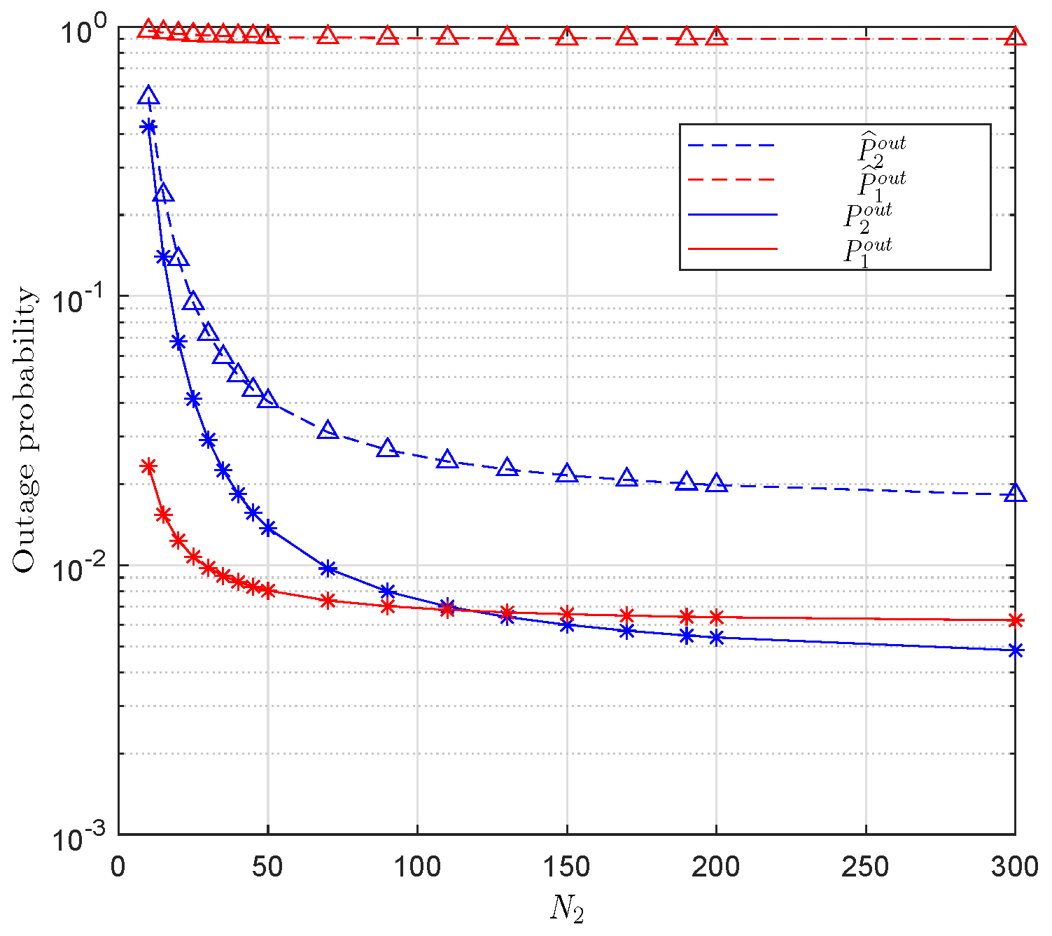
Please note that in all figures that will be presented in this section, the markers represent the results of simulations, while solid lines represent the analytical and asymptotic results under the perfect CSI assumption, and the dashed lines represent the results with imperfect MMSE channel estimation.
5.1. Capacity and Energy Efficiency
In this subsection, we first examine the capacity and the energy efficiency (EE) of both schemes, where EE is defined as . (For simplicity, we only consider transmission energy here, as it is the major component, and we neglect other energy consumption in the system. An exhaustive energy efficiency framework will complement this work in the future.) Figure 2 and Figure 3 show the simulated capacity together with the average and asymptotic capacity for different values of a and b, while Figure 4 and Figure 5 show the energy efficiency for different values of a and b. All results are given for both perfect and imperfect CSI.
Clearly, the asymptotic values presented in Table 1, Table 2, Table 3 and Table 4 can perfectly predict the performance of Scheme 1 and Scheme 2 under perfect and imperfect CSI. In fact, as N grows infinitely large, the capacity when and has no upper bound. In the other cases, as N increases, the capacity increases towards a constant asymptotic value—except for with Scheme 1, where it decreases towards zero. Moreover, as discussed in Section 4.1.1, Scheme 2 outperforms Scheme 1 for all power scaling options when N is large enough. Further, observing Figure 4 and Figure 5, we can conclude that Scheme 2 is the best in terms of energy efficiency when combined with relevant power scaling.
However, in terms of complexity, Scheme 2 is worse than Scheme 1. Hence, for a fair comparison, and in order to get the same complexity, we select different values of N for each scheme in what follows. Let us denote by and the numbers of antennas for Scheme 1 and Scheme 2, respectively. Based on the complexity approximations for channel estimation and precoding for each scheme, and in order to get the same complexity for both schemes, the following constraint is respected:
and
Figure 6, Figure 7, Figure 8 and Figure 9 show the capacity and energy efficiency for both schemes with the same complexity level. We clearly see that with the additional complexity constraint, Scheme 1 now always outperforms Scheme 2 for the perfect CSI condition—except when the power scaling at the relay is very high, i.e., . However, under imperfect CSI, Scheme 2 remains a better choice at the same complexity level for all proposed a and b values.
5.2. Outage Probability
In this subsection, we compare the studied schemes in terms of outage probability, and for space considerations, we limit our analysis to the case of power scaling at the relay, i.e., and . Moreover, in all figures, we assume that both schemes have the same complexity, i.e., the constraints in (59) and (60) are respected. In Figure 10, we first note that the simulation results confirm the accuracy of the analytical expressions obtained in Section 3.1.2, Section 3.2.5, Section 4.1.2, and Section 4.2.3. We conclude that Scheme 1 outperforms Scheme 2 in term of outage probability when assuming the same complexities and a perfect CSI for some numbers of transmitting antennas. Under imperfect CSI, we see that Scheme 2 is always the best.
6. Conclusions
In this paper, we have analyzed the end-to-end capacity, its asymptotic approximation, and the outage probability of an outdoor-to-indoor dual-hop full-duplex mmWave multi-user system for which the transmitting nodes are equipped with massive numbers of antennas while the final users are equipped with single antennas. Two precoding schemes were proposed, and the performance metrics were derived for each scheme under both perfect and imperfect CSI conditions. An approximation of the precoding complexity was also given for each precoding scheme. To respect the power budget allocated to the relay, the normalization coefficient was approximated, capitalizing on the law of large numbers. Monte Carlo simulation results were presented to confirm the accuracy of our analysis. Practical recommendations were formulated at the end of the analysis for both pure performance and for fair performance–complexity trade-off comparisons.
Author Contributions
Conceptualization, N.B., H.C. and M.B.; Data curation, N.B., H.C. and M.B.; Formal analysis, N.B., H.C. and M.B.; Investigation, N.B., H.C. and M.B.; Methodology, N.B., H.C. and M.B.; Project administration, N.B., H.C. and M.B.; Resources, N.B., H.C. and M.B.; Software, N.B., H.C. and M.B.; Supervision, N.B., H.C. and M.B.; Validation, N.B., H.C. and M.B.; Visualization, N.B., H.C. and M.B.; Writing—original draft, N.B., H.C. and M.B.; Writing—review and editing, N.B., H.C. and M.B. All authors have read and agreed to the published version of the manuscript.
Funding
This research received no external funding.
Data Availability Statement
All obtained data in this work is the result of the mathematical calculations detailed in the paper. Supporting simulation scripts can be shared upon request.
Conflicts of Interest
The authors declare no conflicts of interest.
References
- Bounouader, N.; Chafnaji, H.; Benjillali, M. Power Normalization and Precoding for Massive MIMO in Outdoor-to-Indoor mmWave Relaying. In Proceedings of the 6th International Conference on Advanced Communication Technologies and Networking (CommNet), Rabat, Morocco, 11–13 December 2023; pp. 1–7. [Google Scholar]
- Hong, W.; Jiang, Z.H.; Yu, C.; Hou, D.; Wang, H.; Guo, C.; Hu, Y.; Kuai, L.; Yu, Y.; Jiang, Z.; et al. The role of millimeter-wave technologies in 5G/6G wireless communications. IEEE J. Microw. 2021, 1, 101–122. [Google Scholar] [CrossRef]
- Sakaguchi, K.; Yoneda, T.; Iwabuchi, M.; Murakami, T. Mmwave massive Analog relay MIMO. ITU J. Future Evol. Technol. 2021, 2, 43–55. [Google Scholar] [CrossRef]
- Nguyen, N.T.; Nguyen, H.N.; Nguyen, N.L.; Le, A.T.; Nguyen, T.N.; Voznak, M. Performance analysis of NOMA-based hybrid satellite-terrestrial relay system using mmWave technology. IEEE Access 2023, 11, 10696–10707. [Google Scholar] [CrossRef]
- Li, D.; Xu, G.; Gao, M.; Song, Z.; Zhang, Q.; Zhang, W. Performance Analyses of RIS-Assisted Stochastic UAV mmWave Relay Communication System With Moment Matching Estimation. IEEE Wirel. Commun. Lett. 2024, 13, 1198–1202. [Google Scholar] [CrossRef]
- Marzetta, T.L. How much training is required for multiuser MIMO? In Proceedings of the 40-th Asilomar Conference on Signals, Systems and Computers, Pacific Grove, CA, USA, 29 October–1 November 2006; pp. 359–363. [Google Scholar]
- Marzetta, T.L. Noncooperative Cellular Wireless with Unlimited Numbers of Base Station Antennas. IEEE Trans. Wirel. Commun. 2010, 9, 3590–3600. [Google Scholar] [CrossRef]
- Grossman, D. mmWave for Fixed Wireless: What We’ve Learned; Technical Report, Strategy Analytics; Strategy Analytics: Ottawa, ON, Canada, 2022. [Google Scholar]
- Ntontin, K.; Verikoukis, C. Relay-aided outdoor-to-indoor communication in millimeter-wave cellular networks. IEEE Syst. J. 2019, 14, 2473–2484. [Google Scholar] [CrossRef]
- Albreem, M.A.; Juntti, M.; Shahabuddin, S. Massive MIMO detection techniques: A survey. IEEE Commun. Surv. Tutor. 2019, 21, 3109–3132. [Google Scholar] [CrossRef]
- Zhang, Z.; Long, K.; Vasilakos, A.V.; Hanzo, L. Full-Duplex Wireless Communications: Challenges, Solutions, and Future Research Directions. Proc. IEEE 2016, 104, 1369–1409. [Google Scholar] [CrossRef]
- Koc, A.; Le-Ngoc, T. Full-duplex mmWave massive MIMO systems: A joint hybrid precoding/combining and self-interference cancellation design. IEEE Open J. Commun. Soc. 2021, 2, 754–774. [Google Scholar] [CrossRef]
- Osama, I.; Rihan, M.; Elhefnawy, M.; Eldolil, S.; Malhat, H.A.E.A. A review on Precoding Techniques For mm-Wave Massive MIMO Wireless Systems. Int. J. Commun. Netw. Inf. Secur. 2022, 14, 26–36. [Google Scholar] [CrossRef]
- Marzetta, T.L.; Ngo, H.Q. Fundamentals of Massive MIMO; Cambridge University Press: Cambridge, UK, 2016. [Google Scholar]
- Chae, C.B.; Tang, T.; Heath, R.W.; Cho, S. MIMO relaying with linear processing for multiuser transmission in fixed relay networks. IEEE Trans. Signal Process. 2008, 56, 727–738. [Google Scholar] [CrossRef]
- Lee, C.; Chae, C.B.; Kim, T.; Choi, S.; Lee, J. Network massive MIMO for cell-boundary users: From a precoding normalization perspective. In Proceedings of the IEEE Globecom Workshops, Anaheim, CA, USA, 3–7 December 2012; pp. 233–237. [Google Scholar]
- Lin, H.; Zhu, H.; Yang, Y.; Huang, G.; Huang, K.; Chen, Y. Robust Channel estimation for 5G mmWave massive MIMO relay communication systems. In Proceedings of the IEEE 21st International Conference on Communication Technology (ICCT), Tianjin, China, 13–16 October 2021; pp. 289–294. [Google Scholar]
- Eltayeb, M.E. Relay-aided channel estimation for mmWave systems with imperfect antenna arrays. In Proceedings of the IEEE International Conference on Communications (ICC), Shanghai, China, 20–24 May 2019; pp. 1–5. [Google Scholar]
- Tabataba, F.S.; Sadeghi, P.; Pakravan, M.R. Outage Probability and Power Allocation of Amplify and Forward Relaying with Channel Estimation Errors. IEEE Trans. Wirel. Commun. 2011, 10, 124–134. [Google Scholar] [CrossRef]
- Cao, Y.; Liang, X.; Wang, X.; Li, Y.; Fu, Q.; Wang, D.; You, X. Performance of Cell-Free Massive MIMO Under Imperfect Channel State Information and Reciprocity Calibration. IEEE Syst. J. 2023, 17, 4383–4394. [Google Scholar] [CrossRef]
- Niu, Y.; Li, Y.; Jin, D.; Su, L.; Vasilakos, A.V. A survey of millimeter wave communications (mmWave) for 5G: Opportunities and challenges. Wirel. Netw. 2015, 21, 2657–2676. [Google Scholar] [CrossRef]
- Akdeniz, M.R.; Liu, Y.; Samimi, M.K.; Sun, S.; Rangan, S.; Rappaport, T.S.; Erkip, E. Millimeter Wave Channel Modeling and Cellular Capacity Evaluation. IEEE J. Sel. Areas Commun. 2014, 32, 1164–1179. [Google Scholar] [CrossRef]
- Pandey, B.C.; Mohammed, S.K.; Raviteja, P.; Hong, Y.; Viterbo, E. Low complexity precoding and detection in multi-user massive MIMO OTFS downlink. IEEE Trans. Veh. Technol. 2021, 70, 4389–4405. [Google Scholar] [CrossRef]
- Cui, H.; Song, L.; Jiao, B. Multi-pair two-way amplify-and-forward relaying with very large number of relay antennas. IEEE Trans. Wirel. Commun. 2014, 13, 2636–2645. [Google Scholar]
- Coelho, C.A. The generalized integer Gamma distribution: A basis for distributions in multivariate analysis. J. Multivar. Anal. 1998, 64, 86–102. [Google Scholar] [CrossRef]
- Ngo, H.Q.; Larsson, E.G.; Marzetta, T.L. Energy and spectral efficiency of very large multiuser MIMO systems. IEEE Trans. Commun. 2013, 61, 1436–1449. [Google Scholar]
- Hawej, M.; Shayan, Y.R. Low-complexity channel estimation for time division duplex massive multi-user multi-input multi-output systems. IET Commun. 2021, 15, 43–50. [Google Scholar] [CrossRef]
Figure 1.
Adopted system model with massive-MIMO-based outdoor-to-indoor relaying with multiple indoor users.
Figure 1.
Adopted system model with massive-MIMO-based outdoor-to-indoor relaying with multiple indoor users.

Figure 2.
Capacity and asymptotic capacity for different values of a and b, with , , and under perfect and imperfect CSI.
Figure 2.
Capacity and asymptotic capacity for different values of a and b, with , , and under perfect and imperfect CSI.
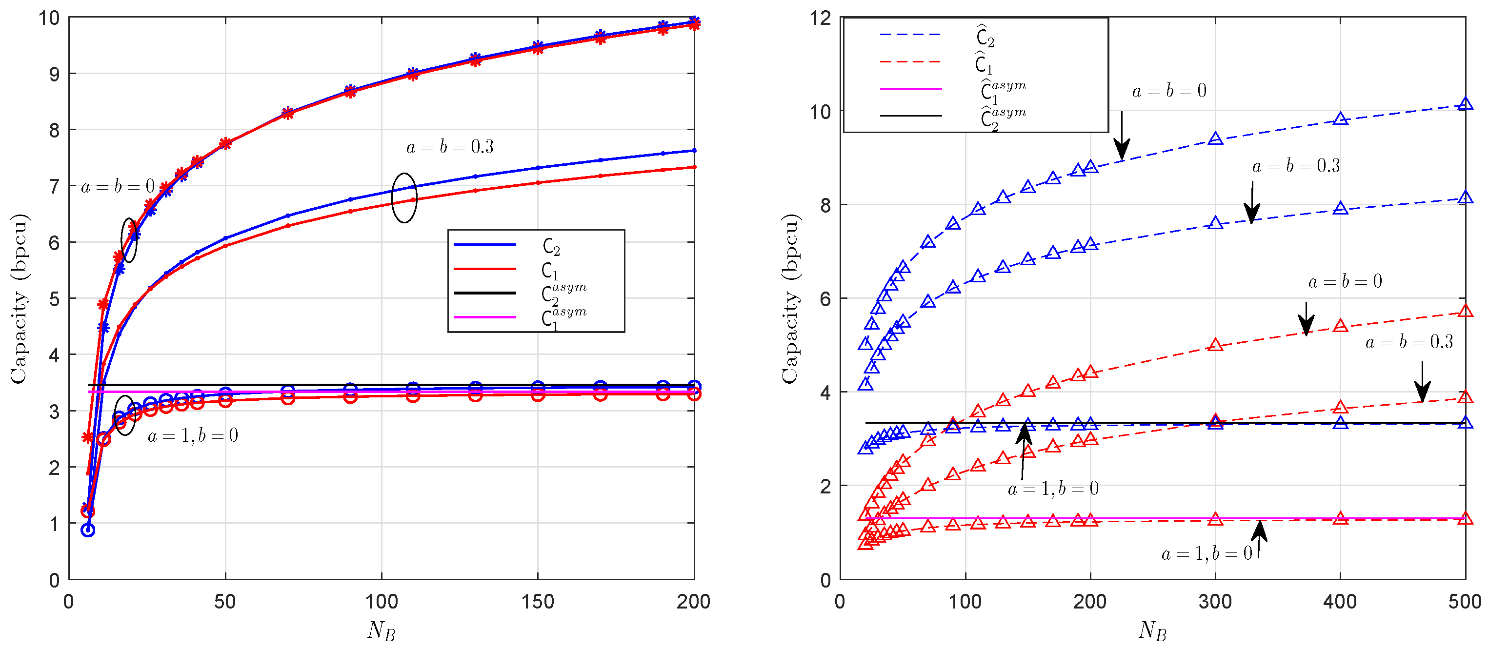
Figure 3.
Capacity and asymptotic capacity for different values of a and b, with , , and under perfect and imperfect CSI.
Figure 3.
Capacity and asymptotic capacity for different values of a and b, with , , and under perfect and imperfect CSI.
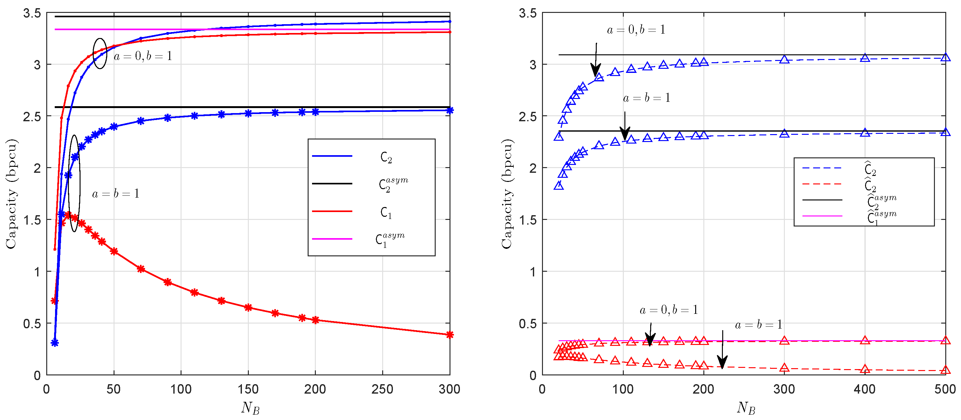
Figure 4.
Energy efficiency for different values of a and b, with , , and under perfect and imperfect CSI.
Figure 4.
Energy efficiency for different values of a and b, with , , and under perfect and imperfect CSI.
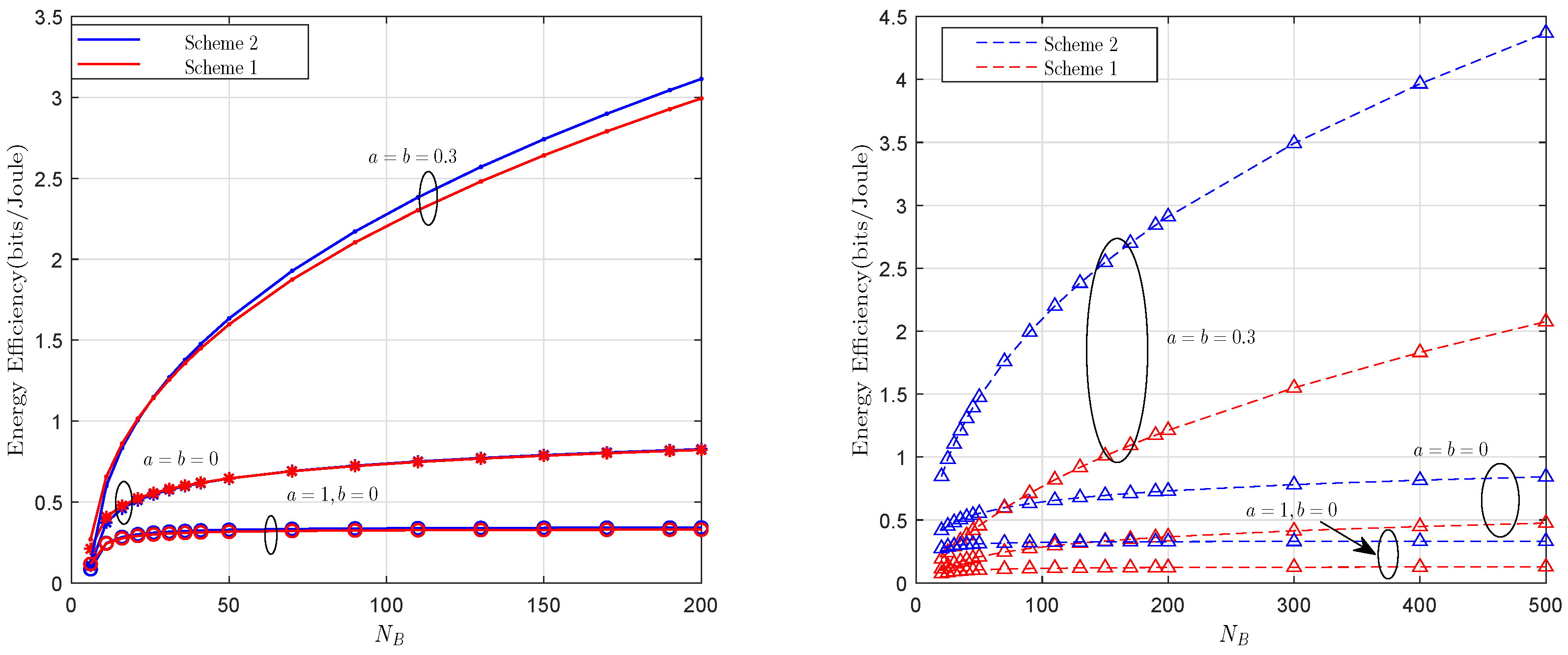
Figure 5.
Energy efficiency for different values of a and b, with , , and under perfect and imperfect CSI.
Figure 5.
Energy efficiency for different values of a and b, with , , and under perfect and imperfect CSI.

Figure 6.
Capacity of Scheme 1 and Scheme 2 at equal complexities for different values of a and b when , , and under perfect and imperfect CSI.
Figure 6.
Capacity of Scheme 1 and Scheme 2 at equal complexities for different values of a and b when , , and under perfect and imperfect CSI.

Figure 7.
Capacity of Scheme 1 and Scheme 2 at equal complexities for different values of a and b when , , and under perfect and imperfect CSI.
Figure 7.
Capacity of Scheme 1 and Scheme 2 at equal complexities for different values of a and b when , , and under perfect and imperfect CSI.
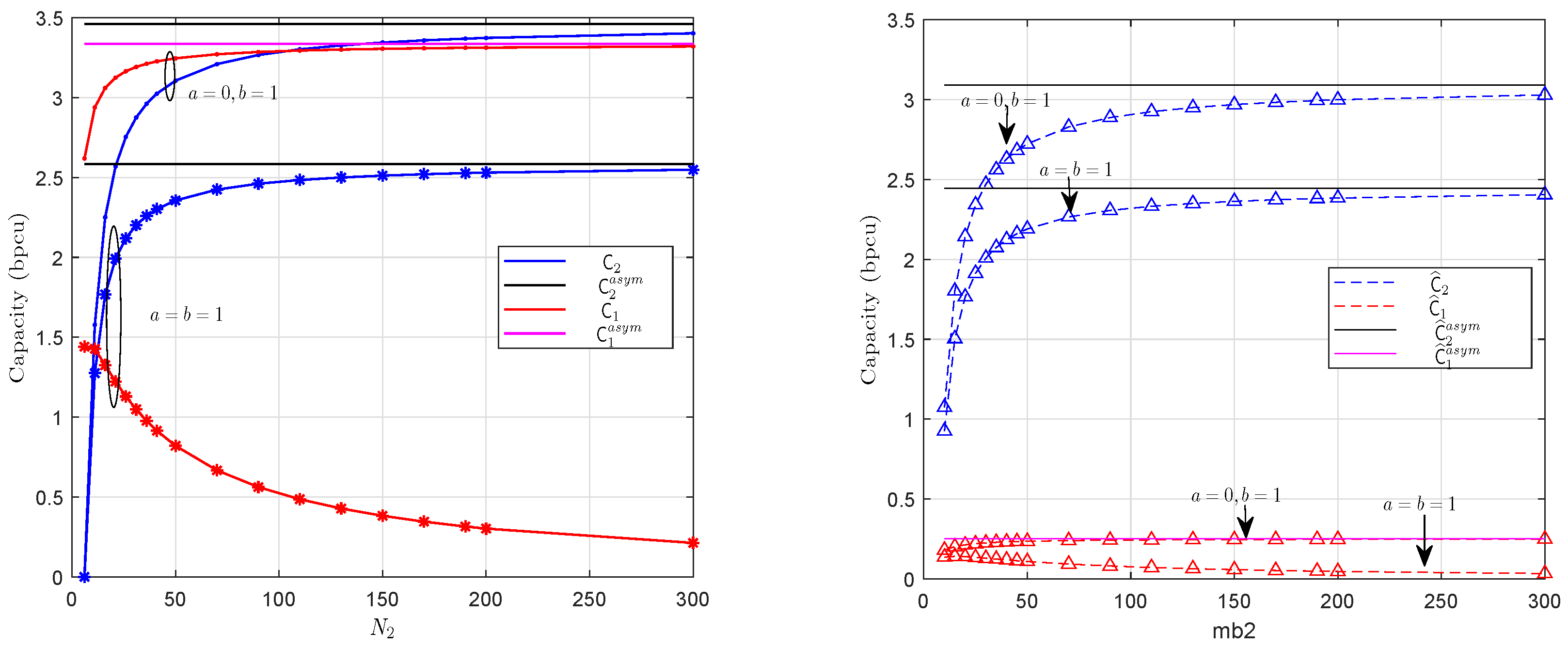
Figure 8.
Energy efficiency of Scheme 1 and Scheme 2 at equal complexities for different values of a and b when , , and under perfect and imperfect CSI.
Figure 8.
Energy efficiency of Scheme 1 and Scheme 2 at equal complexities for different values of a and b when , , and under perfect and imperfect CSI.

Figure 9.
Energy efficiency of Scheme 1 and Scheme 2 at equal complexities for different values of a and b when , , and under perfect and imperfect CSI.
Figure 9.
Energy efficiency of Scheme 1 and Scheme 2 at equal complexities for different values of a and b when , , and under perfect and imperfect CSI.

Figure 10.
Analytical and simulated outage probability assuming the same complexities for and , , , and .
Figure 10.
Analytical and simulated outage probability assuming the same complexities for and , , , and .

Table 1.
Asymptotic SNRs with different power scaling—Scheme 1 and perfect CSI.
| Power Scaling Parameters | Asymptotic SNR () |
|---|---|
| ∞ | |
| , and | |
| and | |
| and | |
| 0 |
Table 2.
Asymptotic SNRs with different power scaling—Scheme 1 and imperfect CSI.
| Power Scaling Parameters | Asymptotic SNR () |
|---|---|
| ∞ | |
| , and | |
| and | |
| and | |
| 0 |
Table 3.
Asymptotic SNRs with different power scaling—Scheme 2 and perfect CSI.
| Power Scaling Parameters | Asymptotic SNR () |
|---|---|
| , | ∞ |
| and | |
| and | |
Table 4.
Asymptotic SNRs with different power scaling—Scheme 2 and imperfect CSI.
| Power Scaling Parameters | Asymptotic SNR () |
|---|---|
| , | ∞ |
| and | |
| and | |
Disclaimer/Publisher’s Note: The statements, opinions and data contained in all publications are solely those of the individual author(s) and contributor(s) and not of MDPI and/or the editor(s). MDPI and/or the editor(s) disclaim responsibility for any injury to people or property resulting from any ideas, methods, instructions or products referred to in the content. |
© 2024 by the authors. Licensee MDPI, Basel, Switzerland. This article is an open access article distributed under the terms and conditions of the Creative Commons Attribution (CC BY) license (https://creativecommons.org/licenses/by/4.0/).
Share and Cite
MDPI and ACS Style
Bounouader, N.; Chafnaji, H.; Benjillali, M. Outdoor-to-Indoor mmWave Relaying with Massive MIMO: Impact of Imperfect Channel Estimation. Electronics 2024, 13, 1857. https://doi.org/10.3390/electronics13101857
AMA Style
Bounouader N, Chafnaji H, Benjillali M. Outdoor-to-Indoor mmWave Relaying with Massive MIMO: Impact of Imperfect Channel Estimation. Electronics. 2024; 13(10):1857. https://doi.org/10.3390/electronics13101857
Chicago/Turabian StyleBounouader, Nawal, Houda Chafnaji, and Mustapha Benjillali. 2024. "Outdoor-to-Indoor mmWave Relaying with Massive MIMO: Impact of Imperfect Channel Estimation" Electronics 13, no. 10: 1857. https://doi.org/10.3390/electronics13101857
Note that from the first issue of 2016, this journal uses article numbers instead of page numbers. See further details here.