Grid-Based Non-Uniform Probabilistic Roadmap-Based AGV Path Planning in Narrow Passages and Complex Environments

Abstract

In this paper, we propose a Grid-based Non-uniform Probability Density Sampling Probabilistic Roadmap algorithm (GN-PRM) in response to the challenges of difficult sampling in narrow passages and low-probability map generation in traditional Probabilistic Roadmap algorithms (PRM). The improved algorithm incorporates grid-based processing for map segmentation, employing non-uniform probability density sampling based on the different attributes of each block to enhance sampling probability in narrow passages. Additionally, considering the computational cost and frequent ineffective searches in traditional PRM algorithms during pathfinding, this paper optimizes the time required for query route planning by altering connection strategies to improve the algorithm’s runtime. Finally, the simulation results indicate that, with a reduction of over 50% in undirected line segments and a reduction of over 85% in runtime, the GN-PRM algorithm achieves a 100% success rate in complex planning scenarios with a sampling point value of K = 500. In comparison, the traditional PRM algorithm has a success rate of no more than 10%, with a sampling point value of K = 500.

1. Introduction

Automatic guided vehicles (AGV) are intelligent industrial transportation devices characterized by their high autonomy, flexibility, programmable control, and adaptability [1]. Currently, they serve as a crucial component in the intelligent and automated production of industries.

In AGV systems, path planning is a paramount aspect [2], serving as a prerequisite for the correct movement of AGV vehicles. The results of path planning determine the intelligence level and availability of AGV vehicles [3]. Various researchers have proposed different methods to address path planning issues, such as the traditional A* [4] and D* [5] algorithms. The A* algorithm combines Dijkstra and BFS algorithms, enhancing search speed through learning a heuristic function. Additionally, drawing inspiration from nature, many researchers have introduced novel algorithms, including artificial potential field [6,7] algorithms, artificial bee colony [8,9], genetic algorithms [10], particle swarm optimization [11], ant colony algorithms [12], and more. With the advancement of research in artificial intelligence and deep learning, numerous researchers have proposed leveraging a Large Language Model (LLM) for robot path planning [13,14,15]. These algorithms, compared to others, require iteration and optimization to find the optimal path, potentially leading to longer times being needed to obtain effective paths in complex environments [16].

In contrast to previous algorithms, path planning methods based on random sampling have been widely applied and researched due to their higher planning speeds [17]. Among these, the most traditional random sampling path planning methods are Rapidly Exploring Random Trees (RRT) [18,19] and Probabilistic Roadmap methods (PRM) [20]. Compared to previous methods, random sampling algorithms use sampled points to describe the free space [21]. The Rapidly Exploring Random Trees (RRT) algorithm randomly selects a free point at each step and employs a separate query process to solve the path planning problem [22]. The PRM algorithm constructs the free space, simultaneously selecting all sampled points and conducting queries [23]. In comparison with the RRT algorithm, the PRM algorithm, by pre-constructing the free space, can rapidly obtain the shortest path. The algorithm primarily consists of two phases: the learning phase and the query phase [24]. The learning phase primarily involves the use of different sets of points to represent the entire workspace, with these points being randomly sampled throughout the workspace. The algorithm also connects each point with all other points, conducting a collision detection, and stores the generated collision-free lines to represent the connected segments of the entire workspace. Consequently, after the learning phase, the original workspace transforms into a workspace composed of freely sampled points and collision-free lines generated by the algorithm. The query phase of the algorithm builds upon the previous step by using a planning algorithm to perform path planning on the generated collision-free lines, creating a connecting line from the starting point to the destination. The PRM algorithm can pre-construct free points and collision-free lines that are tailored to a specific environment, significantly reducing the time required for collision detection and optimizing the efficiency of path planning.

However, due to the PRM algorithm’s reliance on random sampling for free point selection, it exhibits a low success rate in solving path planning problems in narrow passages and complex environments. To enhance the performance of the PRM algorithm, researchers have proposed various methods to optimize the map-learning techniques of free spaces in a narrow passages and complex environments. Boor, V et al. introduced Gaussian sampling [25], which increases the sampling count in narrow passages by transforming obstacle points into free points on the obstacle boundaries through random perturbation. Hsu, D et al. proposed bridge sampling [26,27], determining collision-free midpoints that serve as sampling points in narrow passages. Chen Yan [28] and others suggested a deep-learning-based approach to train and optimize sampling, but these sampling methods often require additional computational efforts to determine the landing positions of the sampling points, which may not meet real-time requirements. Han Chao [29] and colleagues introduced a light node-based sampling method, simulating illumination to sample unsampled areas and ensure the connectivity of the region. While this method effectively meets the requirements of simple narrow passage maps, it exhibits poor adaptability to irregular narrow passages and general maps.

In order to address the issue of prolonged search times for current heuristic and bio-inspired algorithms on large maps, as well as the inadequacy of sampling algorithms in narrow passages, this paper proposes a grid-based non-uniform PRM (GN-PRM) algorithm. By strategizing the point selection across different grids, the algorithm enhances the probability of point selection in narrow passages. Additionally, the connection strategies and methods are optimized to improve the algorithm’s operational speed. We achieved a rapid and robust path planning for AGVs in complex environments on large maps. The primary contributions of this paper are as follows:

• To ensure the connectivity of the sampling graph and increase the number of samples in the narrow passages, we optimize the strategy of extracting sampling points by gridding, identifying, and classifying the features in each grid of the graph. Different sampling strategies are used for different grids. The number of sampling points in open areas is reduced and the number of sampling points in narrow passages is increased, without changing the total number of sampling points, to ensure feasibility in narrow passages.
• In order to accelerate the algorithm’s running speed and better meet the real-time requirements of path planning algorithms, we optimize the connection strategy of sampling points, reduce the generation of undirected line segments by over 50%, and further optimize the path through pruning. Without significantly increasing the length of the route, this approach reduces over 40.9% the time needed to connect collision-free lines during the program, thereby enhancing the algorithm’s operational speed.
• To ensure the optimality of the planned path, we prune and optimize the routes generated in the query phase, reducing the generation of redundant points. The optimized route nodes are reduced by an average of 38.7%, and the route length experiences a reduction of approximately 17.6%.

Section 2 primarily provides an overview of the operation process and principles of the traditional PRM algorithm. Section 3 elaborates on the innovations and improvements made in this paper concerning the GN-PRM algorithm, including grid partitioning, non-uniform probability density sampling methods, and the optimization of route connections and searches. Section 4 demonstrates the optimization results of the improved algorithm through a comparison with the original. Section 5 concludes the entire document.

2. Traditional PRM Algorithm

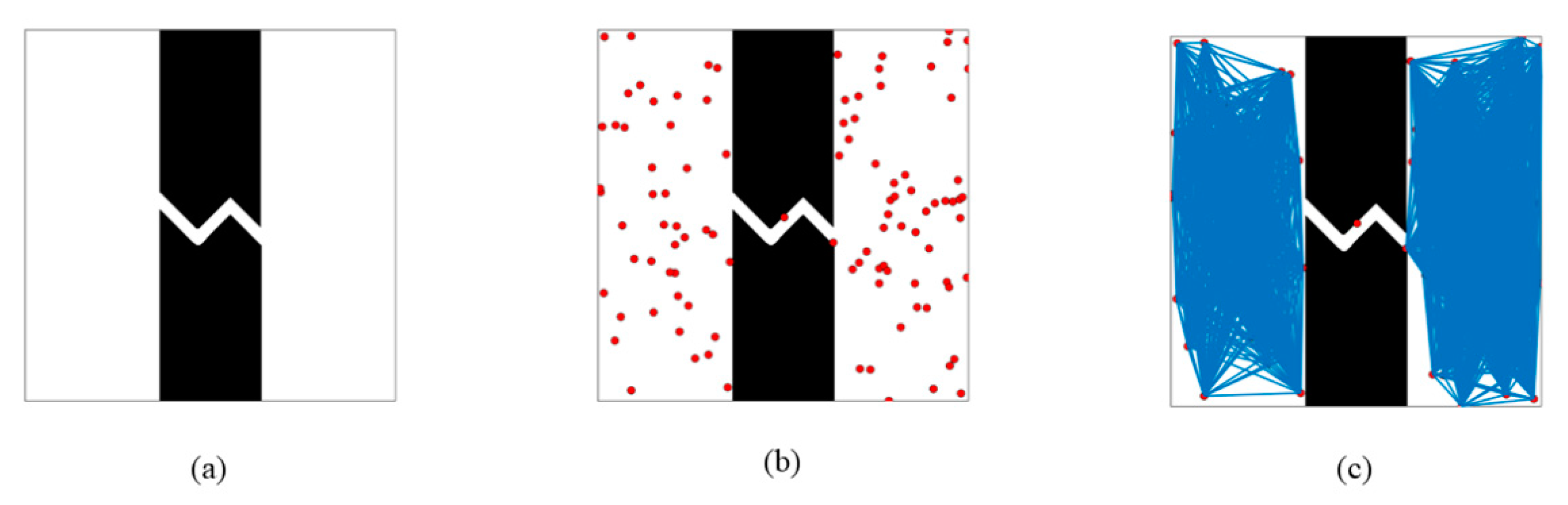
The traditional PRM algorithm is a well-known global path planning algorithm that allows for robots to find a collision-free path from a specified initial position to the corresponding final destination. In the traditional PRM algorithm, the description of free space is directly represented by free points and collision-free line segments. Through this approach, the algorithm can effectively reduce the occupancy of the workspace during path planning. The PRM algorithm primarily consists of a learning phase and a query phase. In Figure 1, (a) illustrates an original map with a size of 500 × 500, (b) and (c) depict the sampling of red points and the connection between undirected blue line segments performed by the traditional PRM algorithm in the learning phase, and (d) shows the algorithm searching all undirected line segments and providing the optimal path in red during the query phase. The specific operations and descriptions of each phase are detailed below.

2.1. The Learning Process

The primary objective during the learning phase is to construct a simplified free space in the workspace through random sampling, which will be utilized for subsequent path planning. During the learning phase, the algorithm primarily has two tasks: sampling points and connecting sampled points to construct undirected line segments. The time complexity of point sampling is typically approximately linear, i.e., $O\left(k\right)$, while the time complexity of constructing undirected line segments is usually approximately $O(k^2)$, where $K$ is the number of sampled points.

Based on the data from the corresponding input map, we can divide the map space $C_s$ into free space $C_{free}$ and obstacle space $C_{obs}$. The operations in the learning phase are mainly as illustrated in Figure 2.

Firstly, the algorithm reads and initializes the map data, dividing the overall space $C_s$ into the free space $C_{free}$ and the obstacle space $C_{obs}$. Subsequently, random sampling points are selected by performing random sampling in the entire space $C_s$, and the sampled points are added to the list of sampling points $C_p$. Finally, the algorithm checks whether the sampling task is complete. If the number of samples $K$ is less than the specified value, the algorithm continues sampling until the task is completed.

Upon completing the description of the space using the set of points, we use collision-free line segments between points to represent effective local paths. These collision-free lines ensure that the robot can navigate the free space. While learning the collision-free lines, the algorithm selects the first free point $P_i(i=1)$ and another free point $P_j(j=1)$ to construct a line segment. Subsequently, collision detection is performed on the learned line segment. If a collision occurs, the segment is discarded, and the process continues to another sampling point $P_i(j=j+1)$ Otherwise, the two endpoints of the path are added to the set of line segments until the entire set of points is traversed. It is worth noting that substantial resources are consumed when learning undirected line segments using this process to traverse the set of points.

2.2. The Query Process

The primary objective of the query process in the PRM algorithm is to leverage the collision-free paths constructed during the learning phase to identify paths between the starting and ending points. By employing local path planning, the algorithm aims to discover an effective path, thereby obtaining a practical route from the initial position to the final destination. Since collision-free local paths are established during the learning process, the search for the optimal path is confined to the set of undirected line segments derived from the learning process, rather than spanning the entire free space.

In the query process of the traditional PRM algorithm, the primary local path planners typically involve A* or Dijkstra algorithms. The Dijkstra algorithm employs the greedy algorithm’s concept by progressively extending the shortest known paths, gradually determining the shortest paths from the starting point to other vertices and ultimately identifying the shortest path to the endpoint. In comparison to the Dijkstra algorithm, the A* algorithm incorporates a heuristic function to determine the optimal path, resulting in greater efficiency in path planning for static workspaces. Therefore, in the query process of the traditional PRM algorithm, the A* algorithm has emerged as the predominant local path planner. When utilizing the A* algorithm to complete the query process, the cost function for evaluating paths is as follows:

$$f\left(x\right)=g\left(x\right)+h\left(x\right)$$

(1)

where, $f\left(x\right)$ represents the estimated total cost, $g\left(x\right)$ denotes the actual cost from the path’s starting point to the current node $x,$ and $h\left(x\right)$ represents the minimum estimated cost from node $x$ to the target endpoint, which is typically calculated using the Euclidean distance. If $g\left(x\right)$ is zero, only $g\left(x\right)$ is effective, and the A* algorithm degenerates into the Dijkstra algorithm. If $h\left(x\right)$ is much larger than $g\left(x\right)$, $g\left(x\right)$ can be approximated to zero, and the A* algorithm degenerates into the BFS algorithm.

The flowchart for the entire query phase is shown in Figure 3.

During the query process, we initially create two lists, the open list and the closed list, to store the parameters of the points being queried. The closed list is used to store points that have already been queried and can be disregarded, while the open list is used to store the free points that need exploration. Next, we identify the overall nearest free points that can form a local path with the initial query point $p_0$ and estimate the cost of these nearest free points according to the formula. Then, we select point $p_1$ with the minimum cost serving as the best-performing point, and remove the current query point $p_0$ from the open list. Finally, we check if the best-performing point $p_1$ is the endpoint. If it has not reached the endpoint, we use the previously selected $p_1$ as the query point $p_0^{\prime }$ for the next iteration, and continue querying the point $p_1^{\prime }$ with the lowest cost around $p_0^{\prime }$ until reaching the endpoint.

Through the aforementioned learning and querying processes, the traditional PRM algorithm can be used in path planning for AGV cars in common environments. However, due to the inherent randomness in the sampling points during the learning process, the completeness of the traditional PRM algorithm is relatively poor. This deficiency becomes more apparent in specific types of maps, such as those containing narrow passages and multiple corners, where it often fails to establish connectivity from the starting point to the endpoint, resulting in path planning failures. A simple solution to this problem is to increase the number of sampling points on the map. However, this inevitably generates a large number of invalid points, leading to an increase in algorithm runtime and the wastage of computational resources. To address these issues, this paper proposes a grid-based non-uniform-sampling optimized PRM algorithm.

3. The Optimized PRM Algorithm

This chapter primarily introduces improvement measures for the GN-PRM algorithm. These enhancements include optimizing the sampling effectiveness within narrow passages in complex, large-scale map environments through non-uniform density sampling with grid-based methods. Additionally, it aims to boost algorithm performance by refining strategies for generating undirected line segments and optimizing the paths obtained through pruning methods.

3.1. Optimized Learning Phase

To fulfill path planning tasks, conventional algorithms initially simplify the real environment into a representative two-dimensional map. Subsequently, they employ the traditional Probabilistic Roadmap (PRM) algorithm to derive the workspace, which is primarily composed of sampling points and collision-free line segments. The sampling points serve as the foundation for the formation of collision-free line segments. Figure 4 illustrates the operation of the traditional PRM algorithm in scenarios involving narrow passages. When confronted with complex environments featuring various narrow passages, it is challenging to obtain free points within these narrow passages using random sampling methods. This challenge stems from the relatively small size of the free space in narrow passages compared to the overall free space in the map, making it arduous to acquire free points through random sampling. Consequently, some narrow passages cannot be adequately represented in the sampled workspace, resulting in path planning failures in complex environments with narrow passages. As shown in Figure 4c, due to the insufficient number of red points taken in narrow passages, the algorithm is unable to plan an effective path from the starting point to the endpoint.

3.1.1. Grid-Based Map Partitioning

We can observe that, during the sampling process in the traditional Probabilistic Roadmap (PRM) algorithm, the probability of sampling points falling in non-narrow passage areas is significantly higher than in narrow passage areas, as non-narrow passage areas are much larger. Consequently, this imbalance in sampling probabilities results in the failure of subsequent path planning. Furthermore, in non-narrow passage areas, there are many points where land in open areas often fails to contribute effectively to later path planning. This implies that the number of sampling points in open areas exceeds the algorithm’s requirements, while the number of sampling points in narrow passage areas is insufficient.

To address this issue, we introduced a preprocessing step for the map before entering the learning phase. Assuming that the current size of the read map space $C_s$ is $height\times width$, and the grid size is $blockSize$, the number of obtainable grids $t$ can be calculated as follows:

$$t=ceil\left(\frac{height}{BlockSize}\right)\times ceil\left(\frac{width}{BlockSize}\right)$$

(2)

After partitioning the grids, we classify each grid. When a grid contains no obstacle points, we consider it an open-area grid and label it as such. If a grid is entirely filled with obstacle points, we consider it an inaccessible grid and label it as an obstacle grid. If the number of obstacle points in a grid is below a low predefined threshold, $thresholdlow$, we classify it as a somewhat open-area grid. If the number of obstacle points in a grid exceeds a higher predefined threshold, $thresholdhigh,$ we identify it as a potentially narrow passage-related grid and label it a dangerous grid. When the number of obstacle points in a grid is below $thresholdhigh$ and above $thresholdlow$, we consider it to potentially represent the edge of an obstacle or the entrance/exit of a narrow passage, labeling it a somewhat dangerous grid.

After partitioning the grids, we classify each grid based on its content. A grid containing no obstacle points is categorized as an open-area grid and labeled accordingly. Conversely, if a grid is entirely occupied by obstacle points, we designate it an inaccessible grid and label it as an obstacle grid. Grids with obstacle points below a predefined lower threshold, $thresholdlow$, are classified as a somewhat open-area grid. In cases where the number of obstacle points in a grid exceeds a higher predefined threshold, $thresholdhigh$, we identify the grid as a potentially narrow passage-related grid and label it as a dangerous grid. Grids with obstacle points below $thresholdhigh$ and above $thresholdlow$ are considered to potentially represent the edge of an obstacle or the entrance/exit of a narrow passage, and we label them as somewhat dangerous grids.

When the map size is 500 × 500, the grid size is 50, $thresholdlow$ is set to ${0.1\times BlockSize}^2$, and $thresholdhigh$ is set to ${0.5\times BlockSize}^2$, the program’s execution results are shown in Figure 5. In Figure 5, the red area represents the identified dangerous grids, the blue area represents somewhat dangerous grids, and the green area represents obstacle grids. It can be observed that the narrow passage areas are effectively identified and marked.

3.1.2. Non-Uniform Probability Density Sampling

After the map is divided into grids, we can adopt different sampling strategies for grids with different attributes to improve the success rate of path planning.

Obstacle grids are entirely occupied by obstacles, rendering them impassable. Consequently, during sampling, these grids are ignored to focus sampling efforts on areas with potential connectivity. No sampling is conducted for obstacle grids to redistribute the sampling probability to other regions.

For open grids, as there are no obstacle points inside the grid, creating a relatively open space, if a large number of points fall into an open grid, redundancy in sampling points within the same grid may occur due to the proximity and the fact that, in most cases, only one sampling point per grid is retained in subsequent query processes. To address this issue and maximize the effectiveness of sampling points, our sampling strategy for open grids is to only take the center point of the grid as a fixed sampling point.

Somewhat dangerous grids share most attributes with open grids, although there are minimal obstacle points inside the grid; therefore, redundancy in sampling points may still occur if a large number of points fall into the open gird. Therefore, the sampling strategy for somewhat dangerous grids is the same as that for open grids, taking the center point as the fixed sampling point.

Since they contain a certain number of obstacle points and are often passages for narrow passages or obstacle boundaries, sampling within dangerous grid points is generally more valuable than in open grids or somewhat dangerous grids. Therefore, we need to increase the sampling probability in such grids. When the total number of sampling points, k, is greater than the number of grids, t, we perform a random sampling for each dangerous grid and then conduct a random sampling for all dangerous grids until a sufficient number of sampling points are obtained. With this sampling method, we represent open and somewhat open grids by extracting center points while ensuring that each dangerous grid has at least one sampling point representing it. Additionally, this approach reduces the sampling frequency for obstacle grids, open grids, and somewhat open grids, thereby increasing the probability of sampling in narrow passages and improving the planning success rate of the PRM algorithm.

3.2. Optimized Query Phase

During the operation of the traditional PRM algorithm, sampling determines the completeness of the entire algorithm, i.e., whether the working space can be expressed through sampling on the original map. Meanwhile, connection and search operations need to be performed on the sampled point set. These two aspects determine the overall speed of the algorithm. To enhance the algorithm’s speed and better meet the real-time path computation requirements, this paper has made corresponding improvements to the connection and optimization strategies in the traditional PRM algorithm.

3.2.1. Optimized Connection Strategy

After sampling, the PRM algorithm needs to connect and store the points in the sampled space to form collision-free line segments. The traditional PRM algorithm typically traverses the entire set of sampled points, testing their connectivity with other points, resulting in a time complexity of $O\left(n^2\right)$. As the number of samples, $k$ increases, the algorithm’s runtime exponentially rises, making it challenging to meet real-time requirements. Compared to the GN-PRM, our algorithm achieves a substantial reduction in the connection of sampling points within open areas through the implementation of a restricted connection radius and variable probability sampling. This reduction contributes to a notable decrease in algorithmic execution time without compromising the completeness of probabilistic algorithms. Consequently, the overall operational speed of the algorithm is enhanced.

During the connection process, it was observed that many undirected line segments connecting points in open areas are, in fact, invalid and suboptimal. They not only occupy space in the point set but also increase the workload for subsequent searches. Therefore, this paper proposes a method to reduce redundant nodes by assigning a circular constraint to sampled points. Assuming the current node coordinates are $\left(x_1,y_1\right)$, this will only connect with coordinates within a circle, centered on the current coordinates with a radius of ‘$distance$’. When the $distance$ is infinite, the algorithm degenerates into the standard connection method in the ordinary PRM algorithm. However, if the $distance$ is too small, this may lead to the loss of valid path solutions.

As the total number of sampled points, k, is greater than the number of grids, t, each grid must contain at least one point to ensure connectivity between grid points. To balance overall algorithm connectivity and the existence of valid paths, this paper sets $distance=1.5BlockSize$. This ensures a certain level of connectivity while allowing for grids in open areas to connect with nearby open grids in eight directions, resulting in a more efficient path. After adding circular constraints, as in the case of the same sample points $K=150$, the comparison of generated undirected line segments is shown in Figure 6. In Figure 6, Red points are PRM sampling points and starting and ending points, blue points are open grid points, yellow points are GN-PRM sampling points and the blue lines are undirected line segments.

The table below presents the number of undirected line segments generated by different algorithms on various maps. All data are presented in

Table 1. Comparison table of connection nodes.

Map	Sampling Count	PRM Nodes	GN-PRM Nodes	Reduce Percentage
1	150	5333.54	2027.4	61.98%
2	150	2494.5	1317.06	47.20%
3	150	4822.84	2168.56	55.03%
4	150	5599.38	2143.92	61.71%
5	150	3711.72	1573.32	57.61%
Average percentage reduction of nodes				56.70%

. The data in the table represent the averages obtained after running each algorithm 50 times on different maps. Through comparison, it can be observed that, in comparison to the traditional PRM algorithm, the algorithm proposed in this paper reduces the number of nodes by 56.7%.

3.2.2. Path Pruning Optimization

By employing the aforementioned optimized query method, we can obtain a reachable path from the initial point to the target point. However, as illustrated in Figure 7, the restriction on the connection between sampled points and other sampled points beyond a certain $distance$ leads to a situation where, on a potentially optimal route, the optimal starting point and the optimal ending point may not be directly connected as they exceed the specified distance. Instead, they can only be indirectly linked through other points, introducing the possibility of redundant points occurring along the entire planned route. Therefore, it is necessary to perform a secondary pruning optimization on the obtained path during the query process.

The path pruning technique is a typical and effective method to optimize the initial path obtained during the query process. The typical path pruning technique is primarily based on the fundamental principle that the sum of two sides of a triangle must be greater than the third side, allowing for for the pruning of redundant nodes on the path. Therefore, path pruning techniques can generate a new, optimized path that closely approximates the shortest path. In the PRM algorithm, the initial path obtained during the query process is primarily described using free points. Consequently, path pruning techniques can reduce the number of free points required to describe the optimal path and optimize the required memory, as illustrated in the Figure 8.

Assuming that the path obtained through the path query method consists of $N$ points denoted as $P_0$, $P_1$, $P_2$,…, $P_N$, we initiate data parameterization by placing the starting point into a new point set and initializing the point marker as $P_{start}=P_0, i=1$. Initially, we connect $P_{start+i}$ with $P_{start}$ and perform collision detection. If the line segment exhibits no collision, $i$ is incremented by 1, and the process is repeated, connecting $P_{start+i}$ with $P_{start}$ and assessing collision. The event of a collision between a point $P_t$ and $P_{start}$ implies that the preceding point $P_{t-1}$ can be directly connected to $P_{start}$. Consequently, all points between $P_{start}$ and $P_{t-1}$ are discarded, $P_{t-1}$ is incorporated into a new set of path points, and the new $P_{start}$ is set as $P_{t-1}$. This process is iterated until a connection is detected between $P_{start}$ and the endpoint. Finally, the endpoint is added to the pruned path point set, completing the pruning.

Figure 9 illustrates a comparison of the paths before and after pruning, with the blue line segments representing the pre-pruning path and the red line segments representing the post-pruning path. Compared to the path before optimization, the pruned path exhibits a reduction in the number of nodes and overall path length.

4. Simulations

4.1. Simulation Simulation Comparison between PRM and GN-PRM

In this section, we primarily evaluate the performance of the optimized PRM path algorithm. The experiment comprises four maps, as illustrated in Figure 10a–d: a regular map, a map with simple narrow passages, a map with complex narrow passages, and a map with irregular narrow passages, respectively. The size of each map is 500 × 500, with the starting point set at (10,10) and the endpoint at (490,490). To ensure the accuracy of our data, each map underwent 10 experiments, and the final data represent the average of these 10 trials. The simulations in this section were conducted on a personal computer with a 3.70 GHz Intel-Core (i5-8400) CPU and 32 GB of memory.

To demonstrate the performance of the optimized sampling algorithm, we conducted a comparative analysis with the traditional PRM algorithm. Each algorithm was executed 50 times, and the planning success rate, average planning time, and average planning length were selected as metrics to compare their merits. Based on the results presented in

Table 2. PRM and GN-PRM simulation data table.

Map	Sampling Count	Success Rate		Average Planning Time (s)		Average Planning Length
		PRM	GN-PRM	PRM	GN-PRM	PRM	GN-PRM
a	150	100%	100%	2.42	0.31	698.04	693.01
	500	100%	100%	23.04	0.87	691.59	688.59
b	150	2%	96%	2.40	0.20	731.98	736.02
	500	28%	100%	22.36	0.90	737.62	719.32
c	150	0%	100%	/	0.17	/	875.68
	500	6%	100%	21.53	0.90	902.19	854.45
d	150	0%	92%	/	0.17	/	737.82
	500	4%	100%	18.74	0.85	740.13	727.55

, the following conclusions can be drawn:

(1) In the regular map (a), both the traditional algorithm and the improved algorithm demonstrate effective path planning. With an increase in the number of sampled points, the learning and query times for both PRM algorithms also increase. However, the optimized PRM algorithm proposed in this paper not only ensures an average planning length that is superior to traditional algorithms but also significantly reduces planning time by minimizing redundant routes, thus improving the algorithm’s real-time performance.

(2) In the maps with simple narrow passages (b), complex narrow passages (c), and irregular narrow passages (d), by comparing the success rates when constructing a free space under the same sampled value (K), our algorithm exhibits a higher successful solution rate than the traditional algorithm. The traditional PRM algorithm struggles to complete route planning when the sampled point number (K) is small, whereas our algorithm maintains a high planning completion rate. As K increases, although the success rate of the traditional PRM algorithm improves compared to smaller K values, it still faces challenges in successfully planning routes.

(3) Through a comparison of the constructed route lengths, it is evident that, despite the improved algorithm discarding some connections between undirected line segments, the optimization through pruning that occurs in the experiments on all four maps consistently results in better average route lengths for the improved algorithm under the same K values.

4.2. Simulation Simulation Comparison between GA and GN-PRM

To analyze and compare the GN-PRM algorithm with other algorithms, we used the GN-PRM and the Genetic Algorithm (GA), using each algorithm 50 times. We used planning success rate, average planning time, and average planning length as key indicators for the comparative analysis between the two algorithms. The maps considered in this comparison consist of two simple maps, one simple narrow passages map and one complex narrow passages map, as illustrated in Figure 11.

The parameters of the experimental platform remain consistent with previous settings. The predefined parameters for the Genetic Algorithm (GA) include the number of iterations and the population size. A larger number of iterations and a larger population generally lead to improved planning effectiveness and a higher planning success rate. However, this improvement comes at the cost of an increased iteration time, resulting in a higher overall time requirement for the algorithm. To strike a balance between time efficiency and success rate, we set the population size of the GA algorithm to 50, with 10 iterations, for an optimal real-time performance in a simple map. In a more complex map, we adjusted the population size to 300 and increased the number of iterations to 25 to enhance the planning success rate. For the GN-PRM algorithm, we consistently set the sampling point parameter as $K=150$. The simulation data are presented in

Table 3. GA and GN-PRM simulation data table.

Map	Success Rate		Average Planning Time (s)		Average Planning Length
	GA	GN-PRM	GA	GN-PRM	GA	GN-PRM
a	96%	100%	1.37	0.19	755.44	719.38
b	100%	100%	1.40	0.19	774.52	693.14
c	80%	98%	10.36	0.19	751.54	727.84
d	2%	100%	12.38	0.14	725.00	732.31

. Based on the data in Table 3, we can conduct an analysis and draw conclusions.

(1) In simple maps (a) and (b), both the Genetic Algorithm and GN-PRM demonstrate an almost 100% success rate in completing trajectory planning. However, given the iterative nature of the GA algorithm, its computational time is relatively high. The GN-PRM algorithm, on the other hand, exhibits an average running time that is more than 80% lower than that of the GA algorithm, showcasing superior real-time performance. Concerning the average planned path length, the GA algorithm, which lacks optimization pruning methods, yields a route approximately 5–10% longer than that of the GN-PRM algorithm.

(2) In a narrow passage map (c), although the success rate of the GN-PRM algorithm remains nearly constant, the success rate of the GA algorithm drops to only 80%. However, due to the extensive iterations and population size in complex maps, the average running time of the GA algorithm is more than 50 times that of the GN-PRM algorithm, rendering it unable to meet the real-time requirements of path planning. In the tightly folded narrow passage map (d), the GA algorithm struggles to plan viable paths, while the GN-PRM algorithm consistently achieves a 100% planning success rate with efficiency.

5. Conclusions

In this paper, we propose a novel GN-PRM algorithm that is designed to effectively address the path planning problem for mobile robots navigating through complex environments with narrow passages. Firstly, we employed a grid-based discretization of the map and assigned labels to each grid point based on the distribution of obstacles, implementing diverse sampling strategies for different labeled grid points to enhance the algorithm’s sampling ability within narrow passages. Secondly, we reduced the generation of free segments by limiting the connections between free points and other excessively distant free points, thereby decreasing the algorithm’s computational overhead and enhancing its operational speed. Thirdly, we utilized pruning techniques to eliminate redundant points from the path, ensuring that, even with the exclusion of certain undirected line segments, the algorithm can still yield shorter paths. Finally, extensive comparative experiments with the original PRM and RRT algorithms demonstrated that our proposed PRM algorithm not only improves planning success rates but also significantly reduces algorithm execution times, effectively addressing path planning challenges in narrow workspace environments. The GN-PRM algorithm can be widely applied in industrial production, distribution logistics for AGVs, wheeled robots, and in other areas. Researchers involved in AGV or robot path planning can refer to our paper for insights, utilizing our grid-based non-uniform probability density sampling method to reproduce the paper’s results or to pioneer new algorithms. The results of this paper are reproducible.

The GN-PRM algorithm proposed in this paper primarily addresses the path planning problem for mobile robots in a globally static state. However, the planned route might not be suitable for the robot’s kinematic model in real-world scenarios, especially when dealing with large turning angles. Furthermore, in practical workspaces, the information regarding complex environments often changes over time. Therefore, integrating the PRM algorithm with other methodologies to achieve enhanced navigation results and address path planning challenges in dynamic environments is a crucial research direction. Combining this algorithm with dynamic window methods, deep learning approaches, and other dynamic obstacle-avoidance methods is a promising research avenue, providing valuable insights for fellow researchers.

References

1. Song, X.; Gao, H.; Ding, T.; Gu, Y.; Liu, J.; Tian, K. A Review of the Motion Planning and Control Methods for Automated Vehicles. Sensors 2023, 23, 6140. [Google Scholar] [CrossRef]
2. Patle, B.K.; Babu, L.G.; Pandey, A.; Parhi, D.R.K.; Jagadeesh, A. A review: On path planning strategies for navigation of mobile robot. Def. Technol. 2019, 15, 582–606. [Google Scholar] [CrossRef]
3. Zafar, M.N.; Mohanta, J.C. Methodology for Path Planning and Optimization of Mobile Robots: A Review. Procedia Comput. Sci. 2018, 133, 141–152. [Google Scholar] [CrossRef]
4. Hart, P.E.; Nilsson, N.J.; Raphael, B. A Formal Basis for the Heuristic Determination of Minimum Cost Paths. IEEE Trans. Syst. Sci. Cybern. 1968, 4, 100–107. [Google Scholar] [CrossRef]
5. Stentz, A. Optimal and efficient path planning for partially-known environments. In Proceedings of the 1994 IEEE International Conference on Robotics and Automation, San Diego, CA, USA, 8–13 May 1994; Volume 4, pp. 3310–3317. [Google Scholar]
6. Cho, J.-H.; Pae, D.-S.; Lim, M.-T.; Kang, T.-K. A Real-Time Obstacle Avoidance Method for Autonomous Vehicles Using an Obstacle-Dependent Gaussian Potential Field. J. Adv. Transp. 2018, 2018, 5041401. [Google Scholar] [CrossRef]
7. Koren, Y.; Borenstein, J. Potential field methods and their inherent limitations for mobile robot navigation. In Proceedings of the 1991 IEEE International Conference on Robotics and Automation, Sacramento, CA, USA, 9–11 April 1991; Volume 2, pp. 1398–1404. [Google Scholar]
8. Yin, J.X. Research and application of artificial bee colony algorithm. Master’s Thesis, Xidian University, Xi’an, China, 2012. [Google Scholar]
9. Artificial bee colony algorithm. Scholarpedia 2010, 5, 6915. [CrossRef]
10. Katoch, S.; Chauhan, S.S.; Kumar, V. A review on genetic algorithm: Past, present, and future. Multimed. Tools Appl. 2021, 80, 8091–8126. [Google Scholar] [CrossRef] [PubMed]
11. Shami, T.M.; El-Saleh, A.A.; Alswaitti, M.; Al-Tashi, Q.; Summakieh, M.A.; Mirjalili, S. Particle Swarm Optimization: A Comprehensive Survey. IEEE Access 2022, 10, 10031–10061. [Google Scholar] [CrossRef]
12. Wang, D.S.; Tan, D.P.; Liu, L. Particle swarm optimization algorithm: An overview. Soft Comput. 2018, 22, 387–408. [Google Scholar] [CrossRef]
13. Zhong, J.; Li, M.; Chen, Y.; Wei, Z.; Yang, F.; Shen, H. A Safer Vision-Based Autonomous Planning System for Quadrotor UAVs with Dynamic Obstacle Trajectory Prediction and Its Application with LLMs. In Proceedings of the IEEE/CVF Winter Conference on Applications of Computer Vision, Waikoloa, HI, USA, 4–8 January 2024; pp. 920–929. [Google Scholar]
14. de Curtò, J.; de Zarzà, I.; Roig, G.; Cano, J.C.; Manzoni, P.; Calafate, C.T. LLM-Informed Multi-Armed Bandit Strategies for Non-Stationary Environments. Electronics 2023, 12, 2814. [Google Scholar] [CrossRef]
15. Song, C.H.; Wu, J.; Washington, C.; Sadler, B.M.; Chao, W.-L.; Su, Y. LLM-Planner: Few-Shot Grounded Planning for Embodied Agents with Large Language Models. In Proceedings of the IEEE/CVF International Conference on Computer Vision, Paris, France, 2–3 October 2023; pp. 2998–3009. [Google Scholar]
16. Pati, C.S.; Kala, R. Vision-Based Robot Following Using PID Control. Technologies 2017, 5, 34. [Google Scholar] [CrossRef]
17. Elbanhawi, M.; Simic, M. Sampling-Based Robot Motion Planning: A Review. IEEE Access 2014, 2, 56–77. [Google Scholar] [CrossRef]
18. Wang, F.; Gao, Y.; Chen, Z.; Gong, X.; Zhu, D.; Cong, W. A Path Planning Algorithm of Inspection Robots for Solar Power Plants Based on Improved RRT. Electronics 2023, 12, 4455. [Google Scholar] [CrossRef]
19. Wang, H.; Li, G.; Hou, J.; Chen, L.; Hu, N. A Path Planning Method for Underground Intelligent Vehicles Based on an Improved RRT* Algorithm. Electronics 2022, 11, 294. [Google Scholar] [CrossRef]
20. Kavraki, L.E.; Svestka, P.; Latombe, J.C.; Overmars, M.H. Probabilistic roadmaps for path planning in high-dimensional configuration spaces. IEEE Trans. Robot. Autom. 1996, 12, 566–580. [Google Scholar] [CrossRef]
21. Mac, T.T.; Copot, C.; Tran, D.T.; De Keyser, R. Heuristic approaches in robot path planning: A survey. Robot. Auton. Syst. 2016, 86, 13–28. [Google Scholar] [CrossRef]
22. Karaman, S.; Frazzoli, E. Sampling-based algorithms for optimal motion planning. Int. J. Robot. Res. 2011, 30, 846–894. [Google Scholar] [CrossRef]
23. Yang, J.; Dymond, P.; Jenkin, M. Practicality-Based Probabilistic Roadmaps Method. In Proceedings of the 2011 Canadian Conference on Computer and Robot Vision, St. Johns, NL, Canada, 25–27 May 2011; pp. 102–108. [Google Scholar]
24. Geraerts, R.; Overmars, M.H. Reachability-based analysis for Probabilistic Roadmap planners. Robot. Auton. Syst. 2007, 55, 824–836. [Google Scholar] [CrossRef]
25. Boor, V.; Overmars, M.H.; Stappen, A.F.v.d. The Gaussian sampling strategy for probabilistic roadmap planners. In Proceedings of the 1999 IEEE International Conference on Robotics and Automation (Cat. No.99CH36288C), Detroit, MI, USA, 10–15 May 1999; Volume 2, pp. 1018–1023. [Google Scholar]
26. Zheng, S.; Hsu, D.; Tingting, J.; Kurniawati, H.; Reif, J.H. Narrow passage sampling for probabilistic roadmap planning. IEEE Trans. Robot. 2005, 21, 1105–1115. [Google Scholar] [CrossRef]
27. Hsu, D.; Tingting, J.; Reif, J.; Zheng, S. The bridge test for sampling narrow passages with probabilistic roadmap planners. In Proceedings of the 2003 IEEE International Conference on Robotics and Automation (Cat. No.03CH37422), Taipei, Taiwan, 14–19 September 2003; Volume 3, pp. 4420–4426. [Google Scholar]
28. Chen, Y.; Yu, J. A Neural Network Method for Path Planning of Mobile Robots in Dynamic Environments Based on Probability Roadmap. Qufu Norm. Univ. (Nat. Sci. Ed.) 2019, 45, 38–42. [Google Scholar]
29. Han, C.; Yang, J. Research on PRM path planning optimization algorithm based on optical node model. J. Qingdao Univ. (Eng. Technol. Ed.) 2022, 37, 36–42. [Google Scholar] [CrossRef]
Figure 1. Traditional PRM algorithm diagram. (a) Original map; (b) sampling map (sampling point k = 150); (c) building line segment map; (d) path planning roadmap.
Electronics 13 00225 g001
Figure 2. Learning phase flowchart.
Electronics 13 00225 g002
Figure 3. Query phase flowchart.
Electronics 13 00225 g003
Figure 4. Schematic of narrow passage sampling. (a) Original map; (b) sampling map (sample point k = 150); (c) path planning failure map.
Electronics 13 00225 g004
Figure 5. Grid annotation map. (a1,a2) Original map; (b1,b2) grid map; (c1,c2) identified grid map.
Electronics 13 00225 g005
Figure 6. Comparison diagram of optimized connection algorithms. (a) PRM sampling map (sample point k = 150); (b) PRM building line segment map; (c) GN-PRM sampling map (sample point k = 150); (d) GN-PRM building line segment map.
Electronics 13 00225 g006
Figure 7. Schematic diagram of missing line segments.
Electronics 13 00225 g007
Figure 8. Pruning program flowchart.
Electronics 13 00225 g008
Figure 9. Pruning effect comparison chart. (a,b) Comparison of different paths on different maps before and after pruning.
Electronics 13 00225 g009
Figure 10. Comparative simulation maps. (a) Regular map; (b) simple narrow passages map; (c) complex narrow passages map; (d) irregular narrow passages map.
Electronics 13 00225 g010
Figure 11. Pruning effect comparison chart. (a) Simple map a; (b) simple map b; (c) simple narrow passages map; (d) complex narrow passages map.
Electronics 13 00225 g011