
The Study of SRM Sensorless Control Strategy Based on SOGI-FLL and ADRC-PLL Hybrid Algorithm
1
School of Electrical and Information Engineering, Jiangsu University of Technology, Changzhou 213001, China
2
Jiangsu Key Laboratory of Power Transmission & Distribution Equipment Technology, Changzhou 213001, China
*
Author to whom correspondence should be addressed.
Electronics 2024, 13(1), 2; https://doi.org/10.3390/electronics13010002
Submission received: 25 October 2023
/
Revised: 7 December 2023
/
Accepted: 16 December 2023
/
Published: 19 December 2023
Abstract
:The inductance model used in traditional sensorless control methods for switched reluctance machines (SRMs) exhibits high-order harmonics. The precision of the motor may be impacted by the buildup of rotor estimate errors caused by these harmonics. To address this issue, this paper proposes a novel method for SRMs that employs a hybrid algorithm combining an enhanced second-order generalized integrator (SOGI)-based frequency-locked loop (FLL) and an active disturbance rejection control (ADRC)-based phase-locked loop (PLL). This approach involves coordinate transformation and parameter identification to reconstruct the motor inductance model. Rotor position errors are calculated using the unsaturated inductance difference method. In order to enhance the accuracy of motor position estimation, a hybrid algorithm is employed to efficiently filter out harmonic errors and mitigate the tremor effect caused by the rotor position differential algorithm. This hybrid algorithm enables the estimate of the motor’s speed and rotor position. A sensorless control simulation model was developed using a 12/8 pole SRM to assess the motor’s performance under varying load conditions. Based on the results obtained, it is established that the application of this method can accurately estimate the rotor’s position and rotational speed and thus improve the performance of position sensorless control. Ultimately, a prototype system for a switched reluctance motor was created, and the effectiveness and feasibility of the proposed control technique were confirmed through experimental validation. This presents an innovative approach to engineering practice.
1. Introduction
The SRM is an innovative electric motor that was derived from DC and AC motors [1,2,3]. This motor effectively integrates the advantages of both and has exceptional startup and speed control capabilities. The SRM works in a lot of different areas, including oil fields, aviation, electric vehicle propulsion, and home appliances [4,5]. The device does not require the utilization of rare-earth minerals, possesses a straightforward design, and exhibits flexibility. Consequently, it holds significant potential for widespread implementation. Position sensors are used in traditional control systems to gather rotor position information. However, employing such a methodology results in an increase in both the dimensions and costs associated with the speed control system, which may possibly undermine its reliability in challenging settings [6]. As a result, the investigation of position sensorless technology for SRMs is of utmost significance [7,8].
Scholars have extensively studied the position sensorless technology of SRMs and proposed various control strategies. The control schemes that are currently available can be divided into several groups [8], including the high-frequency pulse injection method [9,10], the magnetic linkage/current method [11,12,13], the model of inductance method [14,15], and the intelligent control method [16,17,18]. The high-frequency pulse injection method has been widely used during the start-up and low-speed operation phases.
In [17], the point where the inductance intersects in the unsaturated inductance region was used as a feature point. The angle that corresponds to the point where the inductance intersects was measured offline, and then a functional relationship was fitted between the point and the angle. In [19,20], an error-correcting method for inductance feature points is suggested. This is done by measuring the angle of the inductance feature point under different loads and then fitting the function to lower the error caused by the intersection point offset. In [21], a position estimation method using the inductance maximum point as a characteristic point is proposed. The method relies on the property that the current slope of the rotor changes from positive to negative as it passes through the inductance maximum point, and therefore, the inductance maximum point is monitored. However, this method is susceptible to inductance saturation, and the conduction region must pass through the inductance maximum region, resulting in a narrow range of turn-off angle modulation. In [22], a low-cost feature position estimation scheme for SRM drivers is proposed. The method initiates the phase change when the estimated magnetic chain reaches a reference threshold. This method reduces the computational burden on the controller by establishing a functional relationship between the phase current and the magnetic chain. In [23], the position of the rotor can be guessed by finding the spot where the inductance inflection point happens because the rotor and stator overlap. This also lets you figure out the phase change point and the instantaneous torque. In [24], an idea for a sensorless startup system that uses two idle-phase inductance thresholds to make sure that the system works smoothly at all speeds is put forward.
However, since the inductance tends to be asymmetric when the motor is manufactured, there is a certain error in using the special points of the inductance as the characteristic points themselves. In [25], a sensorless control method based on the full-period inductance method is suggested. High-frequency pulses are used to get full-period inductance information, which is then used to estimate the position of the motor rotor in a variety of operating conditions. However, the inductance model obtained by this approach does not consider the electromagnetic saturation situation. In [26], the inductance is first split up, and then the inductance model is made by fitting the second-order rational equation to only the unsaturated inductance region. This approach takes into account the electromagnetic saturation case while simplifying the complex inductance modeling process in the literature [25].
All of the above sensorless control methods require offline measurements to obtain the motor inductance model parameters needed to estimate angular position. This is hard to do on a computer and doesn’t work well in most situations. A neural network-based method for estimating the position of a rotor is suggested in [18,27]. This method doesn’t require a precise mathematical model and can work with the non-linear relationship between the magnetic chain, current, and position to find the position of the rotor. However, it requires accurate training data and a long training time. In [28,29], a region-locked-loop-based position estimation method is proposed that does not require offline measurements and can obtain simplified inductance model information through an online method. However, the method does not consider the problem of rotor estimation error caused by harmonics in the inductance model.
Existing sensorless control methods typically compute speed by differential rotor position operations [30,31]. Nevertheless, the connection points of the inductive partitions may cause substantial position errors, leading to notable speed estimation deviations. While the introduction of a low pass filter (LPF) is a possible method for filtering out some of the noise, it can still result in steady-state errors and a slower response to rapid speed changes. Therefore, it is very necessary to use advanced control theory to improve the steady-state performance and dynamic response of the system [32]. In [33], an improved direct torque control (DTC) method is used, combined with a sliding mode controller (SMSC) and an anti-disturbance sliding mode observer (ADSMO), to greatly reduce the torque pulsations of SRMs. In [34], A simple and effective nonlinear element is introduced into the controller, resulting in improved signal-to-noise performance when dealing with small-amplitude signal tracking.
Aiming towards the conventional inductor model, high harmonics result in imprecise model fitting. The accuracy of the location estimate is likely to be compromised due to the reliance on a complex offline measuring technique and the omission of magnetization saturation considerations. The inductance vector transformation strategy is used in this research to offer a method for online adjustment of reconstructed inductor model parameters. The effectiveness and reliability of this method are shown by means of harmonic analysis.
The conventional approach is to obtain the rotor position by solving the inverse trigonometric function [15]. Nevertheless, the hardware architecture of the processor usually provides more appropriate functionality for performing basic arithmetic and logic operations instead of intricate mathematical operations. A dedicated hardware unit is absent in the processor to efficiently carry out the calculation of the inverse trigonometric function. In contrast, the unsaturated inductance difference method proposed in this paper for calculating rotor position error avoids the need for complex trigonometric function operations and significantly reduces computational effort.
The current method uses position differential to figure out speed, which makes error perturbation stronger in the area where the inductance meets. As a consequence, this causes variations in the estimation of both speed and position. We propose a position sensorless control strategy for a switched reluctance motor (SRM) utilizing a hybrid algorithm of a second-order generalized integrator-based frequency-locked loop (SOGI-FLL) and an active disturbance rejection control-based phase-locked loop (ADRC-PLL). The SOGI-FLL algorithm considerably increases the system’s robustness against external perturbations by filtering and transmitting estimated position errors to the ADRC-PLL module for more accurate rotor position estimation. Finally, modeling and experimentation have validated the efficacy and accuracy of the proposed control mechanism.
2. Overall Control Scheme and Working Mode Analysis
2.1. Introduction to the Overall Control Program
This article selects a three-phase 12/8 SRM as the controlled object for the entire system to achieve reliable sensorless operation. The block diagram of the proposed overall control scheme is shown in Figure 1, which consists of five main components: the PI speed regulator module, the torque distribution function, the current chopping controller (CCC) module, the power inverter module, and the sensorless control module.
Mode 1 parameter identification was initiated to identify the parameters of the phase inductance model online. A high-frequency pulse voltage is injected into the three-phase switching transistors. Currently, the CCC module is disabled. The motor remains stationary and inoperable. The unsaturated inductance can be calculated by determining the resulting response current. The reconstructed inductance model is obtained by the inductance vector coordinate transformation (IVCT) method. The reconstructed inductance model has fewer high harmonics. Next, the parameterization of the reconstructed inductor model is performed to obtain the inductor model parameters.
Switch to Mode 2 for sensorless control after online parameter identification is complete. The CCC module starts working at this time. The difference in inductance between zones is calculated using the reconstructed inductance model. The SOGI-FLL algorithm is used to estimate the rotor angular velocity. The ADRC-PLL algorithm is used to estimate the rotor position. The reconstruction and parameterization of the inductance model and the principles of the sensorless hybrid control algorithm are comprehensively discussed below.
2.2. Analysis of Motor Operating Modes
The drive circuit sends pulse signals to switching tubes Q1 and Q2 when the motor is running. Diodes D1 and D2 are currently inoperative, as shown in Figure 2a. Neglecting nonlinear factors such as mutual inductance between phases and eddy currents, the equation for one-phase voltage balance is as follows:
where is the bus voltage of motor, is the voltage of power switching tubes, is the stator resistance, is the response current of winding, is phase inductance, is the angular velocity of rotor, is the position angle of rotor, and is the turn-on time of power switching tubes.
Switching tubes Q1 and Q2 turn off when the phase winding is deactivated. The winding applies a negative voltage to the bus due to its inductance of the winding. Diodes D1 and D2 provide power to the supply. Negative-voltage freewheeling is shown in Figure 2b. The expression for the equation of the voltage loop is as follows:
The pulse signal frequency is high in the high-frequency injection method, resulting in a low response current. Therefore, the incremental inductance calculated online equals the unsaturated inductance. To obtain the incremental inductance, subtract (1) and (2) as follows:
where is the incremental inductance and .
As a result, the incremental inductance of all three phases is determined by detecting the alteration in response current. This is then used to reconstruct the incremental inductance model.
3. Inductance Model Reconstruction Based on Vector Transformation
Due to the high harmonic content of the obtained incremental inductance, the IVCT method is used for reconstruction. The inductance model reconstruction and parameterization flowchart are shown in Figure 3.
The three-phase inductance of the SRM can be represented as three vectors separated by an electrical angle of 120 degrees, ignoring the asymmetry of the inductance. Construct a new coordinate system by rotating abc counterclockwise by δ radians. As shown in Figure 4, is rotated and converted by δ radians to obtain .
By coordinate rotation, the relationship between the inductance vectors in the old and new coordinate systems can be represented as follows:
where δ is the rotation angle of a new coordinate system and is the inductance of the first coordinate transformation. The first transformed inductance is obtained after coordinate rotation. To simplify the calculation, we take the rotation angle δ as , and Equation (4) can be expressed as:
Under the updated coordinate system , the first reconstructed inductance is normalized in Figure 4. The normalized equation for inductance is provided as follows:
where denote the second coordinate transformation inductance.
The second reconstructed inductance Fourier series model’s other higher harmonic content is insignificant and can be portrayed by the fundamental component with the magnitude of L1 as follows:
where is the number of rotor poles and is the fundamental component of the Fourier expansion.
To determine the magnitude of the primary component, the coordinate system’s inductance is converted to the coordinate system as follows:
where is the amplitude of the -axis and is the amplitude of the -axis.
The normalized estimated L1 value is then obtained as follows:
Using the stored parameters tuned through self-adjustment, the uncertain parameters in the phase inductance derived can be eliminated and normalized as follows:
The process of estimating the fundamental components of the inductance is run only once for the same SRM. The fundamental component of the Fourier expansion in the second reconstructed inductance model is obtained after the estimation. The inductance model is divided by the fundamental component for harmonic reduction, and the inductance model is processed to reduce the 2nd harmonic. The normalized reconstructed inductance model characterizes the relationship between the incremental inductance and the actual angle of the rotor. When calculating the actual rotor angle, the second reconstructed incremental inductance and the estimated fundamental component of the inductance can be substituted into the initial inductance model to calculate the actual rotor angle.
4. Rotor Position Estimation Based on Hybrid Algorithm for SRM
Following the acquisition of reconstructed inductance model parameters through Mode 1, the discrepancy between the anticipated and actual motor position is indirectly determined using the unsaturated inductance difference method. By avoiding the effects of magnetic saturation, this method gives the system the ability to support heavy loads.
The speed of the rotor in the conventional sensorless control approach is calculated using position differentiation. However, this frequently leads to the presence of noise in the speed measurements. To ensure stable motor operation, the improved SOGI-FLL estimates the rotor speed before using the estimated speed to estimate the rotor angular position by the ADRC-PLL.
4.1. Calculation of Rotor Position Error Based on Unsaturated Inductance Difference Method
Since the SRM features a double salient pole structure, alterations in the air gap between the rotor and stator generate fluctuations in magnetoresistance, in turn inducing changes in inductance that correlate with the rotor’s position. This non-linear feature amplifies when the current reaches the saturation point of the core material. The accuracy of the position estimation algorithm may be adversely affected. A schematic diagram of the three-phase inductance in the presence of electromagnetic saturation is shown in Figure 5.
The relationship between inductance and the angular position of the rotor remains virtually constant for currents below 10 A. If the current exceeds 10 A, the inductance will significantly decrease due to the magnetic circuit saturation effect. Only unsaturated inductance values are calculated within the pulse injection region to minimize the negative effect of magnetic circuit saturation on rotor position estimation, as shown in Figure 6. The calculation of the unsaturated inductance can be performed using Equation (3) once the idle phase freewheeling is completed.
Based on the number of unsaturated inductors acquired simultaneously, they are classified into six regions: ΙA, ΙB, ΙC, ΙΙAC, ΙΙBA, and ΙΙCB, as shown in Figure 6.
There is only one unsaturated inductance value in the region-ΙB. The single-phase inductance difference method for the B-phase inductance is designed to obtain the position error of the three-phase 12/8 SRM as follows:
where is the amplitude of , and is the estimated position angle.
When , the amplitude and the error . The estimated position will be the same as the actual position when the position is minimized to zero.
Similarly, Equation (12) provides the error for the remaining intervals.
In the region-ΙΙCB, the inductance of both the c and b phases can be obtained and used to obtain position information. By calculating the double-phase heterodyne, the input signal of the hybrid algorithm in region Ⅱ can be obtained by Equation (13)
The position error is calculated as the difference in inductance between the two phases. Similarly, the error for the remaining intervals is obtained using Equation (14).
Through the above calculation, the position error of the motor rotor is obtained, and the motor speed and position are estimated.
4.2. Improved SOGI-FLL Controller Speed Estimation
The conventional SOGI-FLL algorithm has been refined and optimized to enhance the accuracy of speed estimation and eliminate any steady-state error. The linearized SOGI-FLL-ISPPI can be divided into two components: the SOGI and the integral-separated proportional-integral FLL (FLL-ISP-PI), as shown in Figure 7.
In Figure 7, is the input signal, is the output signal, is the quadrature component of , is the estimation error, is the frequency error, k is the system gain take , is the negative proportional gain, is the initial angular frequency, and is the FLL estimated input signal angular.
4.2.1. The Design and Analysis of SOGI
The rotor position is first sinusoidalized to satisfy the input conditions of the SOGI and a nonlinearization parameter , as shown below:
The transfer functions of the output signal , the quadrature component of the output signal , and the error signal with the input signal of SOGI-FLL are as follows:
The amplitude-frequency characteristic curve of , , and is shown in Figure 8. Obviously, they can be regarded as a bandpass filter, a low-pass filter, and a trap filter, respectively. When , the mean of is zero. The input signal has neither amplitude attenuation nor phase lag compared to the output signal , and the SOGI-FLL is locked in that state. When , the error signal is in phase with the quadrature component of the output signal and the average value of is positive. When , the is in reversed-phase with and the average value of is negative.
Thus, the direction of convergence of is determined by . The integral controller’s negative gain Γ matches the input frequency by shifting the SOGI resonant frequency, with higher Γ resulting in faster FLL convergence. Accurately estimating the speed of the rotor can be achieved by adjusting Γ to stabilize the system at E(s) equal to zero.
4.2.2. The Design and Analysis of FLL-ISP-PI
Set the angular frequency of the input signal to and . By using the Formulas (17) and (18), the transfer functions of the output signal and error signal are shown as follows:
The addition of a negative gain Γ to the integral controller enables the SOGI resonant frequency to approach the input frequency . The relationship between the negative gain Γ and the regulation time of the FLL system is illustrated below.
The adjustment of the FLL finally stabilizes the system at , which results in an accurate evaluation of the speed of the rotor. It is necessary to specify the initial resonant frequency to avoid insufficient attenuation of due to low-pass filtering and to prevent it from influencing the convergence of the FLL.
The integral separation term is implemented to prevent overshoot caused by the integral gain. The integral gain is only effective when the error is below the setpoint and ultimately reduces the steady-state error. In order to avoid FLL overshooting and the appearance of steady-state errors while achieving fast convergence to the resonant frequency, SOGI-FLL with attenuated integral-separated PI is proposed, as shown in Figure 7. The estimated speed is expressed as follows:
where , , and are constants, and are taken as 120, 65, and 5, is used to increase the convergence rate of the FLL and reduce the overshoot, and determines the rate at which it decays to zero. is the switching coefficient of the integral term, and the steady state error caused by the integral term is eliminated according to is shown as follows:
where is the threshold of error.
4.3. Improved ADRC-PLL Controller Position Estimation
The second-order ADRC controller can effectively minimize the impact of perturbations on system performance and improve the dynamic performance of the system compared with the traditional PI control. The ADRC consists of three components: the tracking differentiator (TD), the extended state observer (ESO), and the nonlinear state error feedback law (NLSEF). Its fundamental structure is illustrated in Figure 9. The estimates , , and represent the system output , the differential term of the system output , and the total disturbance . denotes the system gain.
4.3.1. The Design of ESO
In order to reduce the error in the position estimation system, it is necessary to observe the position estimation value of the SRM rotor. As shown in Figure 10, the ESO system is designed to obtain the position, velocity, and total disturbance by observing the predicted rotational speed obtained by SOGI-FLL. Observations are fed into the system, compensated, and adjusted in a timely manner to increase system robustness and further improve dynamic performance.
The expression of ESO is as follows:
where is the output of the system, is the rotor predicted angle observation signal, is the rotor angular velocity observation signal, is the disturbance observation signal, is the error between the predicted and actual angle, , , and are the observer error feedback gain, where , , , and are the bandwidths of the state observers, and is the nonlinear function, which can be expressed as:
where is the tracking factor, is the filtering factor used to set the error threshold, and is the error signal.
4.3.2. The Design of NLSEF
To enhance the precision and stability of the system, the NLSEF is created by amalgamating the anticipated angle, angular velocity, and system disruption data monitored by ESO, as outlined below.
where the system has gain coefficients and , which are around , , is the bandwidth of the controller, and is the damping ratio of the system. As a rule of thumb, and .
5. Simulation Studies and Experimental Verification
5.1. Simulation Studies
5.1.1. Motor Control Simulation Model Construction
In order to verify the feasibility of the proposed non-inductive control scheme, a three-phase 12/8 SRM is taken as the research object. Maxwell software is utilized to reconfigure the flux characteristics and torque features of the SRM. The simulation experiment platform is built in Matlab/Simulink for simulation experiment verification. The relevant structural parameters of the SRM prototype are shown in Table 1.
The proposed new method and the traditional sensorless control method [30] were compared and simulated using electromagnetic parameters obtained from Maxwell. The results were then verified in Simulink.
In the simulation, the current chopper controller is operated in a control mode with a pulse injection frequency of 10 kHz and a duty cycle of 33%. The bus voltage is set to 60 V and the rated motor power is 1.5 kW.
5.1.2. Verification and Analysis of Harmonic Suppression for Reconstructed Inductance Models
The harmonic analysis of the inductance before and after reconstruction is depicted in Figure 11. The figure reveals that prior to reconstruction, the DC inductance possessed the greatest share of DC and fundamental components. In addition, the second harmonic component cannot be ignored. Directly ignoring the harmonics above the second harmonic will lead to the inaccuracy of the conventional sensorless control method.
After the vector coordinate transformation, it is equivalent to the difference operation of the two-phase inductance. Therefore, the coordinate-transformed inductor removes the DC component as well as some of the higher harmonics. However, the second harmonic component after coordinate transformation is as high as 16.7%, so its impact on the system cannot be disregarded directly.
After normalization, is similar to , with a small percentage of dc inductance and higher harmonics above the 3rd order. The 2nd harmonic in is reduced to about 4.39%. Apart from the DC inductance component, the maximum amplitude ratio of the higher harmonic components to the fundamental component amplitude is less than 1/25. Thus, the higher harmonics may be disregarded, and the reconstructed inductance can be represented by its fundamental component.
Figure 12 displays the phase inductance under a light load (2 N·m) and a rotational speed of 400 r/min. It also presents the simulated inductance waveforms before and after the inductance coordinate transformation. In Figure 12, a harmonic component is present in the ascending region of inductance with a distinctive burr. The inductance waveform reconstructed in Figure 12b exhibits smooth, continuous sine wave behavior with a specific frequency and amplitude within the inductance drop region.
In summary, using the Coordinate Vector Transformation technique to reconstruct the inductor serves to mitigate the adverse effects of nonlinearity and electromagnetic saturation, thereby reducing the higher-order harmonic components within the system. As a result, the system stability is improved.
5.1.3. Simulation and Analysis of Sensorless Control Strategy
- (1)
- Simulation analysis of motor speed
The motor speed is set at 400 r/min. When the motor is running at full load, we use the conventional position estimation scheme based on the linear region method [30]. The velocity waveform that was measured shows significant pulsations and has a maximum error of 47.6 r/min, as shown in Figure 13.
The reason is that the traditional velocity estimation scheme calculates the velocity by differentiating the position. Based on the linear zone method, the position estimation scheme might be distorted at the inductor intersection, which will make the pulses of the velocity estimation stronger when differentiating.
In contrast, the proposed hybrid control strategy in this paper results in a nearly linear actual velocity waveform. Compared to the traditional method, there is no apparent noise or interference, resulting in smoother operation.
The proposed SOGI-FLL method can filter the position errors obtained above. Controlling the regulation time by adjusting the parameter Γ in Equation (21) not only reduces the pulsation of the velocity estimation but also enhances the stability and reliability of the system.
- (2)
- Simulation analysis of motor rotor position estimation
To further validate motor rotor position estimation accuracy, this study measures motor waveforms under light load and full load operating conditions. The simulated waveforms obtained from the traditional linear zone method [30] and the proposed method in this paper are then compared and analyzed.
The motor is configured to have a load of 2 N·m and a speed of 400 r/min under light load conditions. Figure 14 and Figure 15 exhibit the simulation waveforms of the control scheme using the linear zone methodology and the proposed hybrid algorithm.
Figure 14a depicts the simulated three-phase current waveforms, with a current chopping threshold of approximately 10 A. Additionally, the magnitude of the injected pulse current varies based on the inductance transformation. Figure 14b shows the simulated waveforms of the three-phase inductance, and the maximum value of the phase inductance is about 2.34 mH.
Figure 14b displays the simulated waveforms of the three-phase inductance. The maximum value of the phase inductance measures around 2.34 mH. Figure 14c,d presents a comparison between the predicted and actual positions, along with the resulting position error graphs. The graphs illustrate a positional discrepancy of roughly 2.1 degrees when employing the linear zone approach, with the majority of the discrepancy centered around the intersection of inductance.
The simulated waveforms produced by the proposed control scheme are illustrated in Figure 15. The current chopping threshold depicted in Figure 15a indicates approximately 12 A. The simulated waveforms of the three-phase inductance are exhibited in Figure 15b, and the inductance value calculation takes place solely when the winding current falls below the threshold. It is noticeable from Figure 15c,d that the maximum angular error with the control scheme advocated in this paper is approximately 1.3°.
The motor is set to a load size of 5 N·m with a speed of 400 r/min, resulting in its full load state. Figure 16 illustrates the simulation waveform of the control scheme utilizing the linear zone method, while the hybrid-free algorithm proposed within this paper is demonstrated in Figure 17.
Figure 16a displays the simulated waveforms of a three-phase electric current, revealing the threshold value of the current chopper to be approximately 20 A. Figure 16b portrays the simulated waveforms of three-phase inductance, indicating that the inductance model undergoes deformation due to the on-phase current in the rising inductance area that surpasses the critical saturation current. Figure 16c,d displays a comparison between predicted and actual positions, as well as position error graphs. The analysis calculates the position error between actual and linear zone method positions to be approximately 9.3°. Concentrated error predominantly occurs at the intersection of inductance.
The simulated waveforms using the control scheme proposed in this paper are shown in Figure 17. The current chopping threshold in Figure 17a is about 20 A. Figure 17b shows the simulated waveforms of the three-phase inductance, where the calculation of the inductance value is carried out only when the on-phase current is less than the critical saturation current, and the region belongs to is determined according to the number of regional inductance values. It can be seen in Figure 17c,d that the maximum angular error with the control scheme proposed in this paper is about 2.7°, which is overall smoother.
- (3)
- Simulation analysis of torque variations and disturbances
In order to simulate the actual physical torque variations and disturbances in the results, the effect of motor load jumps on system stability is simulated in the following section. With the motor running smoothly at 400 rpm, a step response signal is applied, and the system load jumps from 2 N·m to 5 N·m and back again. As shown in Figure 18, the motor speed is quickly stabilized by keeping it stable, and the rotor position estimation error is 3.8 degrees. Since the method improves the operation ability under load conditions, it can still achieve good estimation accuracy in the case of load change or external disturbance.
The hybrid algorithm presented in this paper effectively reduces position estimation error by considering current sampling perturbations and electromagnetic saturation, leading to system error. Indirect measurement helps avoid the cumbersome calculation of inverse trigonometric functions in traditional techniques, which ultimately enhances the robustness of the sensorless control system. Additionally, the method effectively filters and estimates rotor speed while reducing position estimation errors, thereby enhancing the overall filtering performance.
Based on the above analysis, it is evident that the hybrid algorithm proposed in this paper offers more precise estimates of rotor position angle compared to the conventional control scheme in light load conditions. Furthermore, it can accurately and smoothly estimate the rotor position angle while remaining independent of electromagnetic saturation under full-load conditions. This provides even greater accuracy compared to the conventional control scheme.
5.2. Experimental Verification
To investigate the practicality of the suggested control approach in engineering, we use a three-phase 12/8 SRM as the subject of research. We create an experimental apparatus for SRM position sensor-less control, as depicted in Figure 19. The SRM controller employs TI’s TMS320F28335 chip as the control core, and the load side utilizes permanent magnet (PM) synchronous motors. The power converter consists of a three-phase asymmetric half-bridge circuit. Through the use of the Tektronix TBS2000B oscilloscope and A622 oscilloscope probe (Tektronix, Beaverton, OR, USA), one can acquire the current measurement and estimate the waveform of the rotor position.
To confirm the precision of the rotor position estimation findings of the control approach introduced in this document during uniform speed operation, a photoelectric encoder is implemented on the mentioned experimental platform to detect the rotor’s present position. The discovered rotor location is then contrasted with the predicted location, resulting in the estimation error of the rotor position. The study’s experimental parameters are detailed in Table 2. The obtained experimental results are analyzed and verified under various operating conditions.
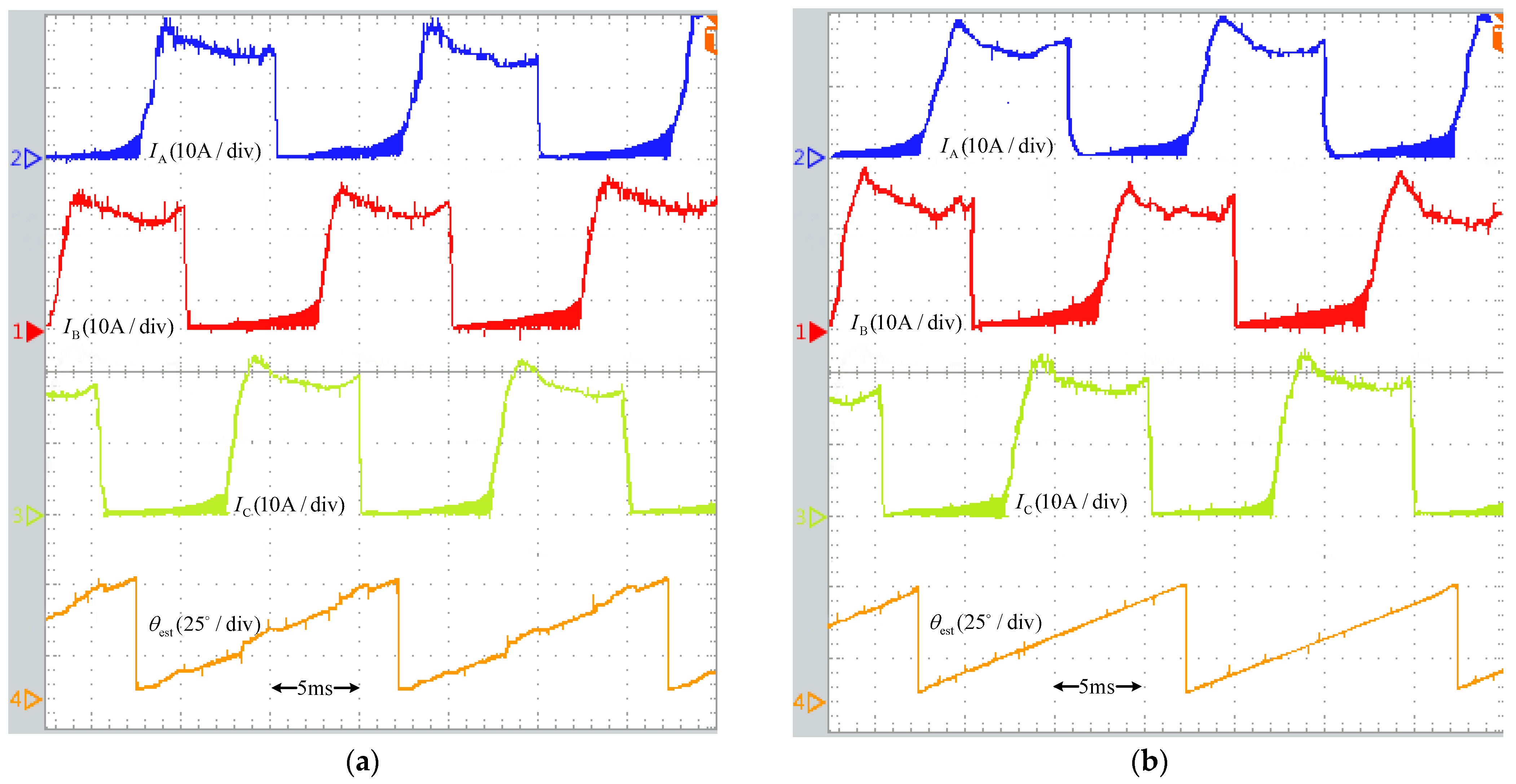
The speed of the SRM is set to 400 r/min with a load of 2 N·m. Figure 20a displays the traditional method’s waveform, which reaches a pinnacle of approximately 12 A, and the position sensor comparison yields an estimated angular error of about 3.6 degrees. On the other hand, Figure 20b depicts the waveform of the hybrid algorithm proposed in this paper, with a peak current of around 13 A and an estimated angular error of about 2.5 degrees.
From Figure 20, it can be seen that when the engine speed is set to 400 rpm and the motor is under a light load of 2 N·m. The waveforms of the traditional method and the proposed method in this paper are more similar and both have high accuracy. Therefore, in the light load scenario, the position estimation method of the proposed scheme and the traditional method both have better performance.
Figure 21a shows the waveform of the conventional approach with an approximate peak value of 20 amps and an estimated angular error of 5.8 degrees compared to the actual position of the position sensor method. Figure 21b illustrates the proposed hybrid algorithm, achieving a peak current of around 20 A and an estimated angular error of 2.7 degrees.
From Figure 21, it can be seen that the conventional method shows obvious jitter at the inductance junction when the motor speed is set to 400 r/min and a heavy load of 5 N·m is applied. Meanwhile, the waveform accuracy of the proposed method in this paper remains high. Therefore, the position estimation method of the proposed scheme has better performance compared to both the conventional methods in heavy load scenarios.
Table 3 compares the average position estimation error of the proposed control strategy and the linear zone control strategy with different loads. Overall, the experimental results align with the simulation and analysis results.
The systematic comparison of the proposed method with the typical traditional sensorless starting methods is presented in Table 4. By comparison with a scheme that does not utilize this paper’s proposed method, this approach yields more precise rotor position estimation in a wider load range.
6. Conclusions
This paper introduces an innovative control strategy tailored for the low-speed stage of a Switched Reluctance Motor (SRM) without relying on a position sensor. The proposed approach integrates coordinate transformation and inductance parameter identification to reconstruct the inductance model. The estimation of position error is calculated using an unsaturated inductance differential method. The SOGI-FLL algorithm can filter the estimated position error signal and output it to the ADRC-PLL module. The ADRC-PLL module can estimate the rotor position more accurately according to the estimated speed and external disturbance after filtering. The motor speed estimate is smoother, and the position estimation is improved by combining the SOGI-FLL and ADRC-PLL algorithms.
Both experimental and simulation results validate the effectiveness of the proposed method. By reducing the computational load associated with conventional anti-triangular functions, the approach presented here significantly improves the precision of rotational position estimation. Furthermore, it addresses challenges posed by current measurement errors and other interference sources, enhancing the overall robustness of the system. Importantly, the proposed method successfully mitigates the impact of magnetic saturation on position estimations, ensuring high-precision performance under varying load conditions.
In conclusion, the developed hybrid algorithm, leveraging the improved SOGI-FLL and ADRC-PLL, demonstrates its capability for achieving sensorless control at low speeds in SRMs. The introduced inductive reconfiguration effectively reduces higher harmonics in the model, contributing to a smoother and more accurate estimation of rotor position and speed. Experimental results affirm the feasibility and efficiency of the proposed control strategy.
Author Contributions
Algorithm design, F.N. and W.Z.; algorithm design, W.Z.; coding and testing, W.Z. and F.N.; design and manufacture of the control system, W.Z. and B.L.; article review and proofreading, W.Z. and Y.B.; funding acquisition, W.Z. All authors have read and agreed to the published version of the manuscript.
Funding
This work was supported by the Changzhou Science and Technology Support Project (CE20235045), Open subject of Jiangsu Province Key Laboratory of Power Transmission and Distribution (2021JSSPD12), National Natural Science Foundation of China (61903166) and Graduate practice innovation program of Jiangsu University of Technology (XSJCX22_57).
Data Availability Statement
All important data are included in the manuscript.
Conflicts of Interest
The authors declare no conflict of interest.
Nomenclature
| The incremental inductance | |
| The first coordinate transformation inductance | |
| The second coordinate transformation inductance. | |
| The fundamental component of the Fourier expansion. | |
| The amplitude of the or -axis | |
| The normalized reconstructed inductance | |
| The negative proportional gain | |
| The initial angular frequency | |
| The frequency error | |
| The rotor position error of actual and estimated | |
| The amplitude of the rotor position error | |
| The estimated position angle | |
| The actual position angle | |
| The number of rotor poles | |
| The threshold of error | |
| The switching coefficient of the integral term | |
| The rate at which it decays to zero | |
| The rotor predicted angle observation signal | |
| The rotor angular velocity observation signal | |
| The disturbance observation signal |
References
- Chaibet, A.; Boukhnifer, M.; Ouddah, N.; Monmasson, E. Experimental Sensorless Control of Switched Reluctance Motor for Electrical Powertrain System. Energies 2020, 13, 3081. [Google Scholar] [CrossRef]
- Ge, L.; Burkhart, B.; Doncker, R.W.D. Fast Iron Loss and Thermal Prediction Method for Power Density and Efficiency Improvement in Switched Reluctance Machines. IEEE Trans. Ind. Electron. 2020, 67, 4463–4473. [Google Scholar] [CrossRef]
- Bilgin, B.; Howey, B.; Callegaro, A.D.; Liang, J.; Kordic, M.; Taylor, J.; Emadi, A. Making the Case for Switched Reluctance Motors for Propulsion Applications. IEEE Trans. Veh. Technol. 2020, 69, 7172–7186. [Google Scholar] [CrossRef]
- Cheng, H.; Liao, S.; Yan, W. Development and Performance Analysis of Segmented-Double-Stator Switched Reluctance Machine. IEEE Trans. Ind. Electron. 2022, 69, 1298–1309. [Google Scholar] [CrossRef]
- Lan, Y.; Benomar, Y.; Deepak, K.; Aksoz, A.; El Baghdadi, M.; Bostanci, E.; Hegazy, O. Switched Reluctance Motors and Drive Systems for Electric Vehicle Powertrains: State of the Art Analysis and Future Trends. Energies 2021, 14, 2079. [Google Scholar] [CrossRef]
- Wang, G.; Valla, M.; Solsona, J. Position Sensorless Permanent Magnet Synchronous Machine Drives—A Review. IEEE Trans. Ind. Electron. 2020, 67, 5830–5842. [Google Scholar] [CrossRef]
- Xiao, D.; Filho, S.R.; Fang, G.; Ye, J.; Emadi, A. Position-Sensorless Control of Switched Reluctance Motor Drives: A Review. IEEE Trans. Transp. Electrif. 2022, 8, 1209–1227. [Google Scholar] [CrossRef]
- Tang, X.T.; Sun, X.D.; Yao, M. An Overview of Position Sensorless Techniques for Switched Reluctance Machine Systems. Appl. Sci. 2022, 12, 3616. [Google Scholar] [CrossRef]
- Pasquesoone, G.; Mikail, R.; Husain, I. Position Estimation at Starting and Lower Speed in Three-Phase Switched Reluctance Machines Using Pulse Injection and Two Thresholds. IEEE Trans. Ind. Appl. 2011, 47, 1724–1731. [Google Scholar] [CrossRef]
- Gan, C.; Chen, Y.; Sun, Q.; Si, J.; Wu, J.; Hu, Y. A Position Sensorless Torque Control Strategy for Switched Reluctance Machines With Fewer Current Sensors. IEEE/ASME Trans. Mechatron. 2021, 26, 1118–1128. [Google Scholar] [CrossRef]
- Sun, X.; Tang, X.; Tian, X.; Wu, J.; Zhu, J. Position Sensorless Control of Switched Reluctance Motor Drives Based on a New Sliding Mode Observer Using Fourier Flux Linkage Model. IEEE Trans. Energy Convers. 2022, 37, 978–988. [Google Scholar] [CrossRef]
- Cai, H.; Han, Y.J.; Jiang, Y.J.; Luo, Z.X.; Liao, J.L. Flexible Sensorless Position Control of Switched Reluctance Motors considering Both Embrace Design and Magnetic Saturation. Front. Energy Res. 2022, 10, 822021. [Google Scholar] [CrossRef]
- Wang, Y.; Ma, Z.; Bahari, M. Position Estimation Method for Switched Reluctance Motors Based on Magnetic Flux Modulation. IEEE Sens. J. 2023, 23, 10395–10403. [Google Scholar] [CrossRef]
- Kim, J.H.; Kim, R.Y. Online sensorless position estimation for switched reluctance motors using characteristics of overlap position based on inductance profile. IET Electr. Power Appl. 2019, 13, 456–462. [Google Scholar] [CrossRef]
- Cai, J.; Zhang, X.; Peng, X.; Yan, Y.; Deng, Z. A Hybrid Sensorless Starting Strategy for SRM With Fault-Tolerant Capability. IEEE Trans. Transp. Electrif. 2023, 9, 2444–2452. [Google Scholar] [CrossRef]
- Kolluru, A.K.; Malligunta, K.K.; Teja, S.R.; Reddy, C.R.; Alqahtani, M.; Khalid, M. A novel controller for PV-fed water pumping optimization system driven by an 8/6 pole SRM with asymmetrical converter. Front. Energy Res. 2023, 11, 1205704. [Google Scholar] [CrossRef]
- Kuang, S.; Zhang, X.; Liu, P.; Zhang, G.; Zhang, Z. Sensorless Control Method for Switched Reluctance Motors Based on Locations of Phase Inductance Characteristic Points. Trans. China Electrotech. Soc. 2020, 35, 4296–4305. [Google Scholar]
- Cai, Y.; Wang, Y.; Xu, H.; Sun, S.; Wang, C.; Sun, L. Research on Rotor Position Model for Switched Reluctance Motor Using Neural Network. IEEE/ASME Trans. Mechatron. 2018, 23, 2762–2773. [Google Scholar]
- Zhang, L.; Liu, C.; Wang, Y.; Zhang, Y. Position Sensorless Technology of Switched Reluctance Machines Based on Double Variable Current Thresholds. Proc. Chin. Soc. Electr. Eng. 2014, 34, 4683–4690. [Google Scholar]
- Li, M.; Chen, X.; Ren, X.; Li, Y. Sensorless Control of Switched Reluctance Motors Based on Typical Positions of Three-Phase Inductances. Proc. Chin. Soc. Electr. Eng. 2017, 37, 3901–3908. [Google Scholar]
- Xu, A.; Ren, P.; Chen, J.; Zhu, J. Rotor Position Detection and Error Compensation of Switched Reluctance Motor Based on Special Inductance Position. Trans. China Electrotech. Soc. 2020, 35, 1613–1623. [Google Scholar]
- Banerjee, R.; Sensarma, P. Low-Cost Realization of Feature Position Estimation Scheme for Switched Reluctance Motor. IEEE Trans. Power Electron. 2023, 38, 2850–2854. [Google Scholar] [CrossRef]
- Kim, J.-H.; Kim, R.-Y. Sensorless Direct Torque Control Using the Inductance Inflection Point for a Switched Reluctance Motor. IEEE Trans. Ind. Electron. 2018, 65, 9336–9345. [Google Scholar] [CrossRef]
- Cai, J.; Liu, Z.Y.; Zeng, Y. Aligned Position Estimation Based Fault-Tolerant Sensorless Control Strategy for SRM Drives. IEEE Trans. Power Electron. 2019, 34, 7754–7762. [Google Scholar] [CrossRef]
- Cai, J.; Deng, Z. Sensorless Control of Switched Reluctance Motors Based on Full-Cycle Inductance Method. Trans. China Electrotech. Soc. 2013, 28, 145–154. [Google Scholar]
- Fang, G.; Scalcon, F.P.; Volpato Filho, C.J.V.; Xiao, D.; Nahid-Mobarakeh, B.; Emadi, A. A Unified Wide-Speed Range Sensorless Control Method for Switched Reluctance Machines Based on Unsaturated Reluctance. IEEE Trans. Ind. Electron. 2023, 70, 9903–9913. [Google Scholar] [CrossRef]
- Mese, E.; Torrey, D.A. An approach for sensorless position estimation for switched reluctance motors using artifical neural networks. IEEE Trans. Power Electron. 2002, 17, 66–75. [Google Scholar] [CrossRef]
- Xiao, D.; Ye, J.; Fang, G.; Xia, Z.; Li, H.; Wang, X.; Nahid-Mobarakeh, B.; Emadi, A. Induced Current Reduction in Position-Sensorless SRM Drives Using Pulse Injection. IEEE Trans. Ind. Electron. 2023, 70, 4620–4630. [Google Scholar] [CrossRef]
- Xiao, D.; Ye, J.; Fang, G.; Xia, Z.; Wang, X.; Emadi, A. A Regional Phase-Locked Loop-Based Low-Speed Position-Sensorless Control Scheme for General-Purpose Switched Reluctance Motor Drives. IEEE Trans. Power Electron. 2022, 37, 5859–5873. [Google Scholar] [CrossRef]
- Cai, J.; Deng, Z. Unbalanced Phase Inductance Adaptable Rotor Position Sensorless Scheme for Switched Reluctance Motor. IEEE Trans. Power Electron. 2018, 33, 4285–4292. [Google Scholar] [CrossRef]
- Cai, J.; Liu, Z. An Unsaturated Inductance Reconstruction Based Universal Sensorless Starting Control Scheme for SRM Drives. IEEE Trans. Ind. Electron. 2020, 67, 9083–9092. [Google Scholar] [CrossRef]
- Fortuna, L.; Frasca, M.; Buscarino, A. Optimal and Robust Control: Advanced Topics with MATLAB®; CRC Press: Boca Raton, FL, USA, 2021. [Google Scholar]
- Sun, X.; Wu, J.; Lei, G.; Guo, Y.; Zhu, J. Torque ripple reduction of SRM drive using improved direct torque control with sliding mode controller and observer. IEEE Trans. Ind. Electron. 2020, 68, 9334–9345. [Google Scholar] [CrossRef]
- Bucolo, M.; Buscarino, A.; Fortuna, L.; Gagliano, S. Can Noise in the Feedback Improve the Performance of a Control System? J. Phys. Soc. Jpn. 2021, 90, 075002. [Google Scholar] [CrossRef]
Figure 1.
Schematic diagram of the proposed sensorless control scheme.

Figure 2.
Driver circuit operating mode for SRM Driver circuit operating mode for SRM. (a) Positive voltage excitation; (b) Negative voltage freewheeling.
Figure 2.
Driver circuit operating mode for SRM Driver circuit operating mode for SRM. (a) Positive voltage excitation; (b) Negative voltage freewheeling.
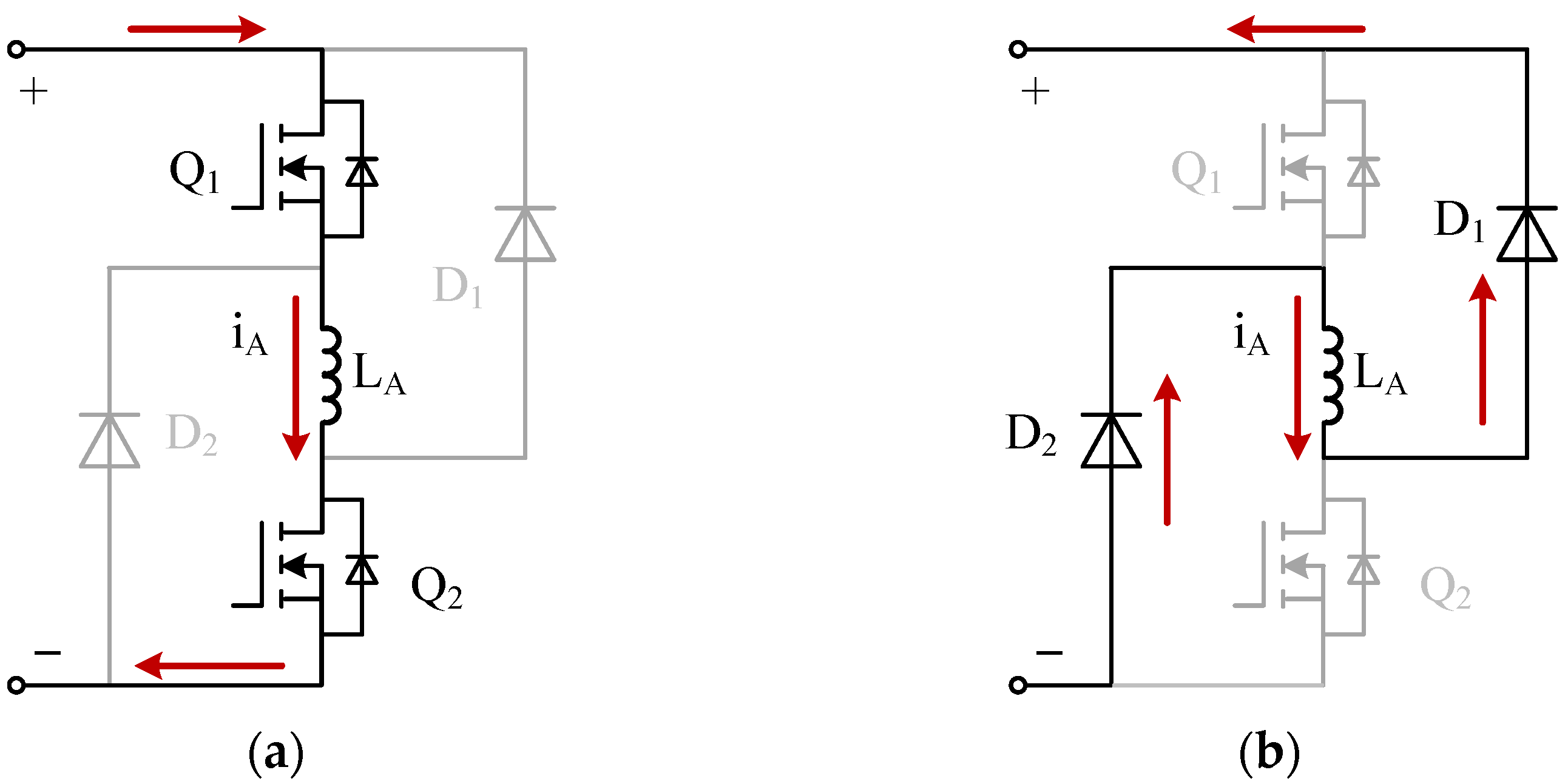
Figure 3.
Inductance model reconstruction and parameterization flowchart.
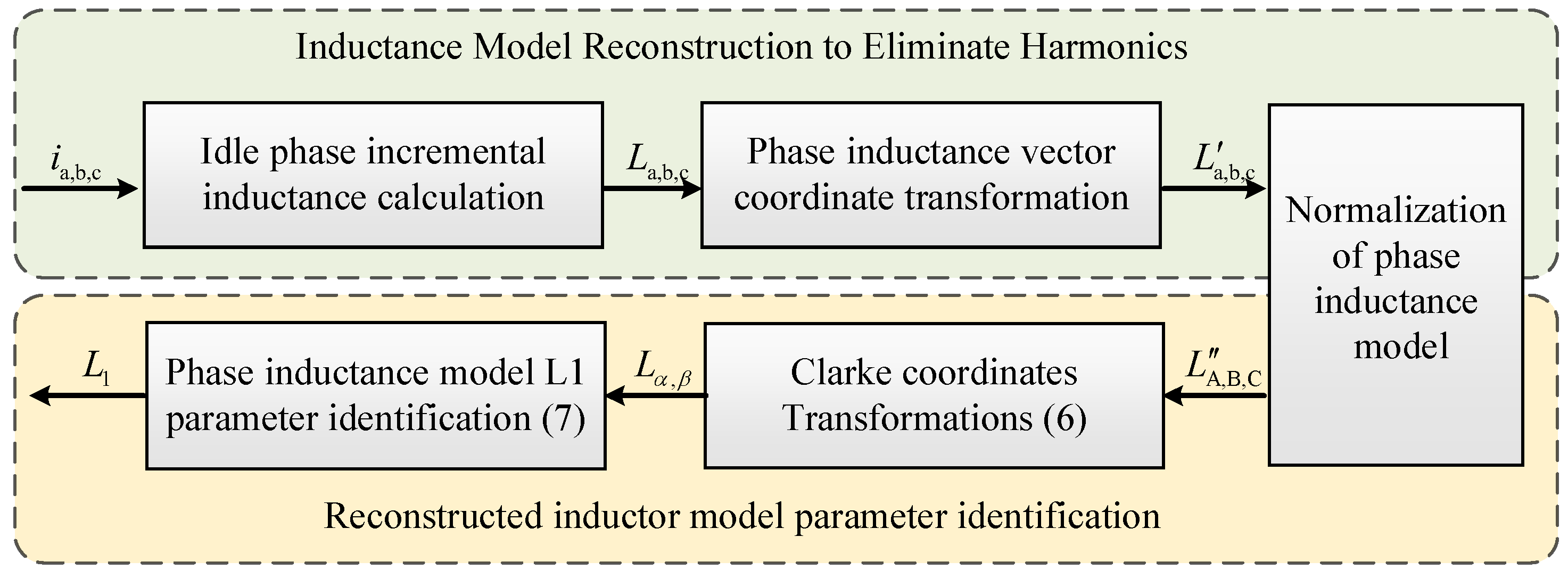
Figure 4.
Inductance vector rotation coordinate transformation.

Figure 5.
Schematic diagram of three-phase inductance considering motor magnetic circuit saturation.
Figure 5.
Schematic diagram of three-phase inductance considering motor magnetic circuit saturation.

Figure 6.
Unsaturated inductor partition difference method schematic diagram.
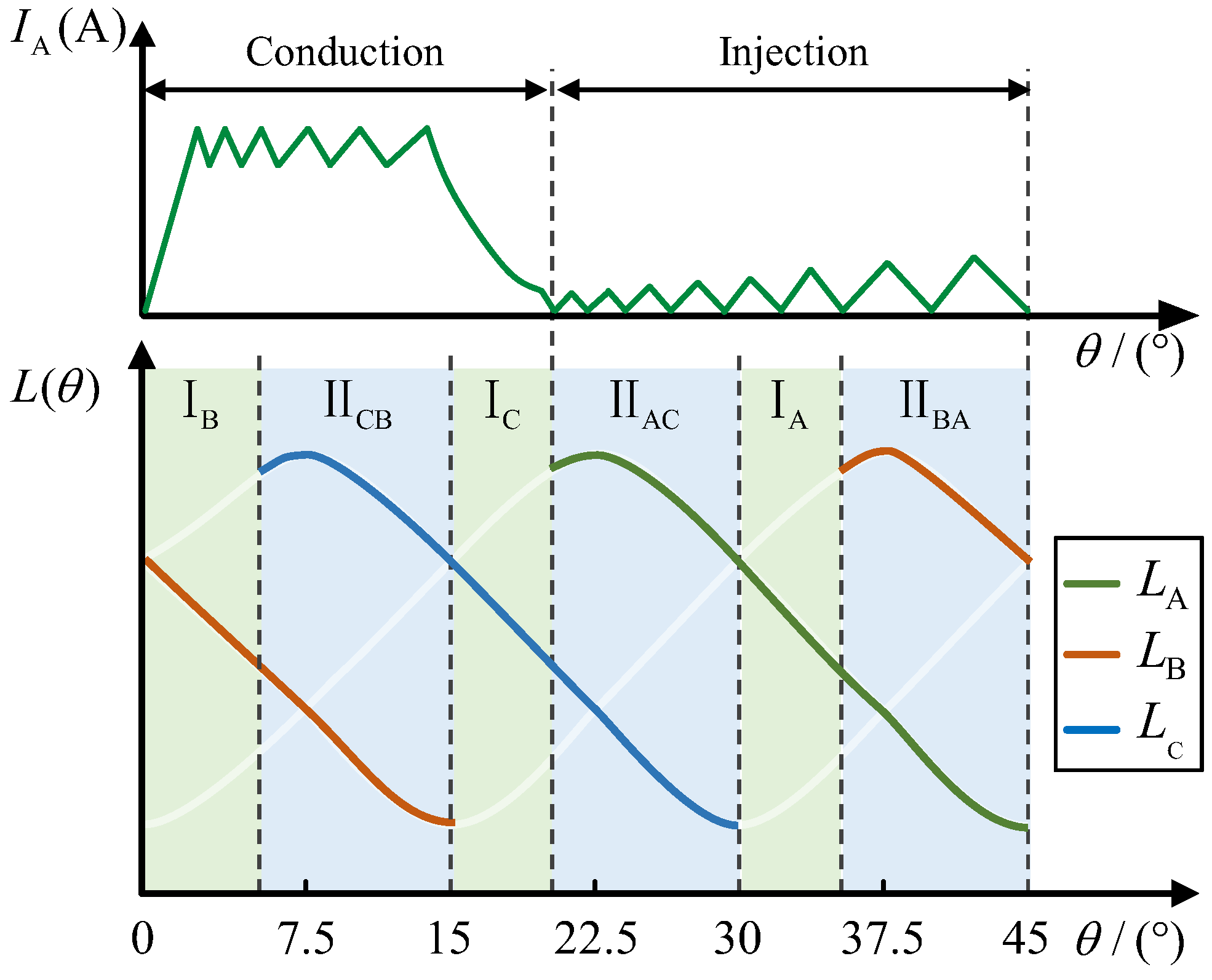
Figure 7.
Linearization model of the proposed SOGI-FLL-ISPPI.
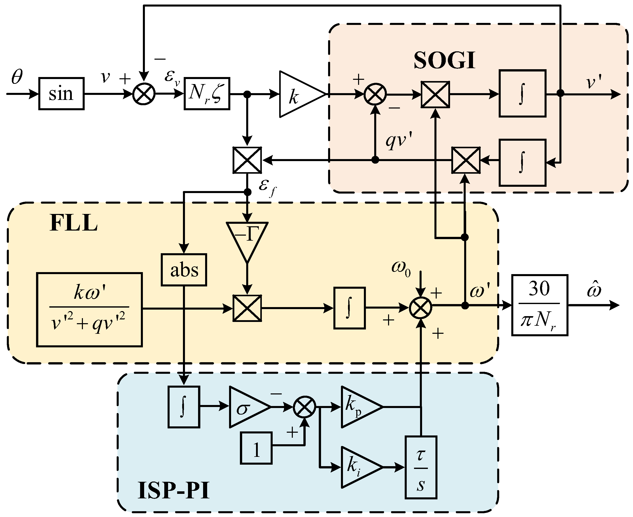
Figure 8.
Bode diagram of the proposed SOGI-FLL.
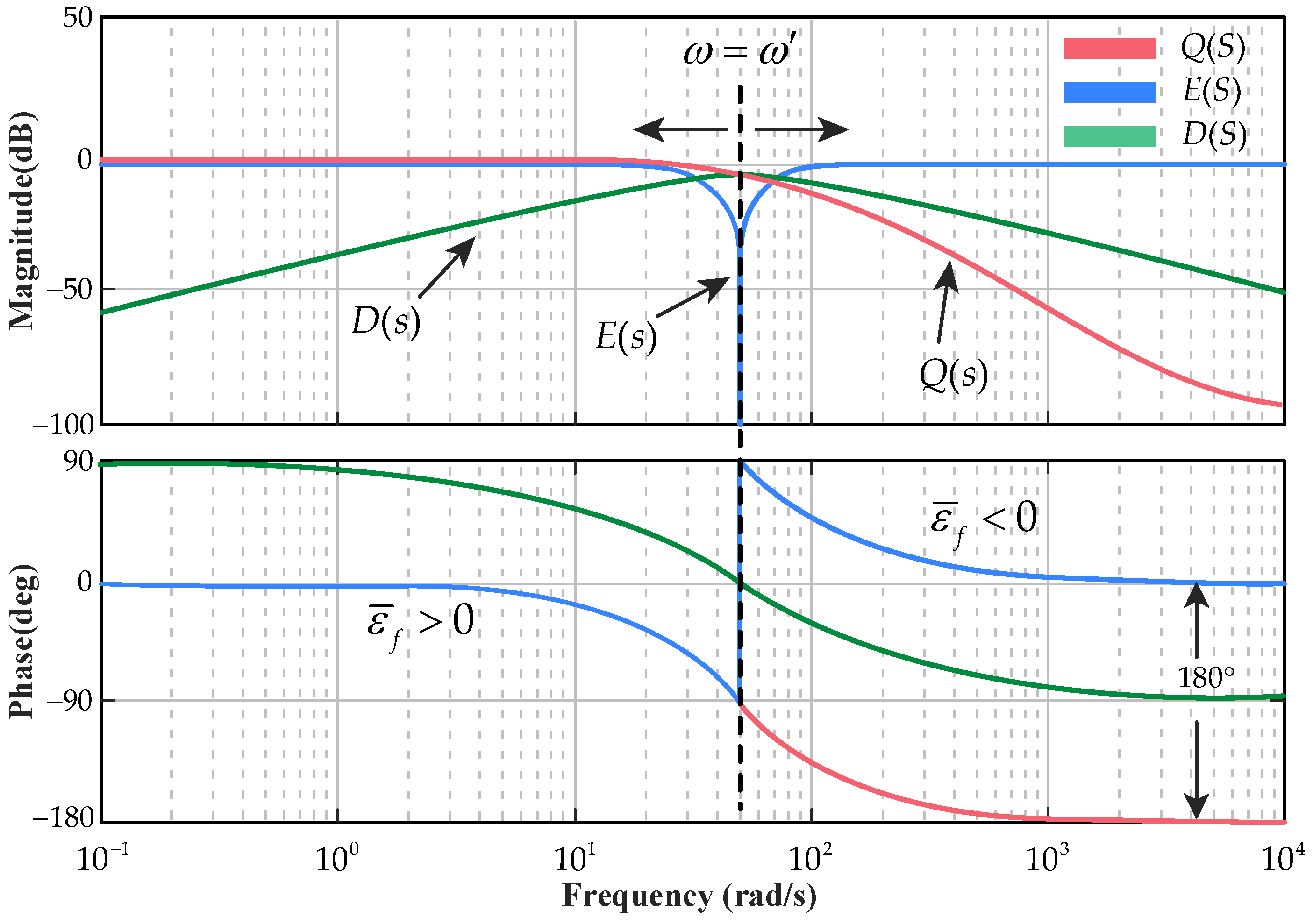
Figure 9.
Linearization model of the proposed ADRC-PLL.
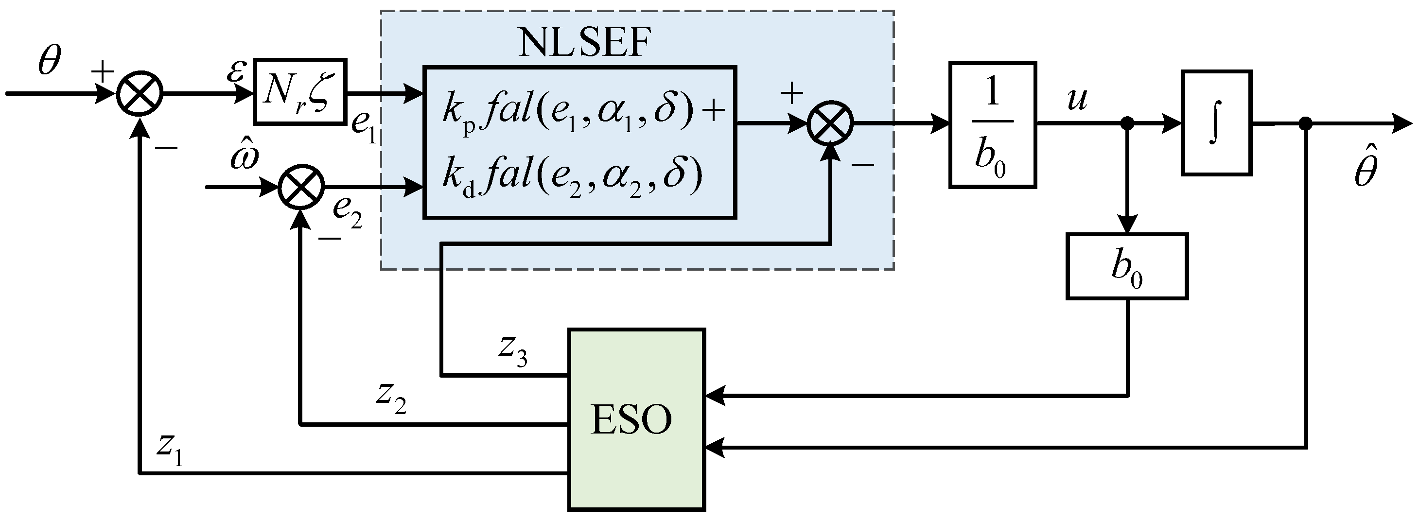
Figure 10.
Expansion state observer structure.
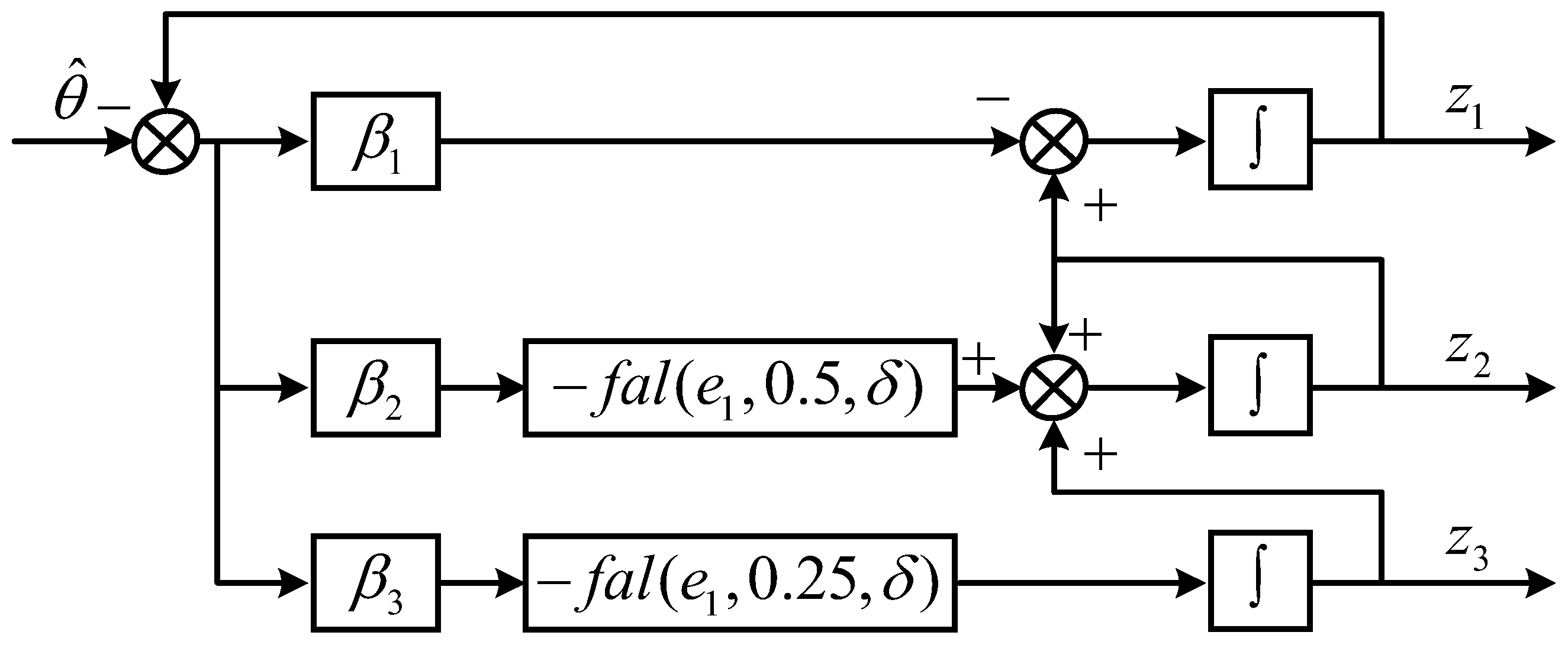
Figure 11.
Inductance coordinate transformation harmonic analysis diagram.

Figure 12.
Simulated waveforms before and after inductor coordinate transformation. (a) Three-phase inductance value (light load 400 r/min). (b) Coordinate transformed three-phase inductance (light load 400 r/min).
Figure 12.
Simulated waveforms before and after inductor coordinate transformation. (a) Three-phase inductance value (light load 400 r/min). (b) Coordinate transformed three-phase inductance (light load 400 r/min).
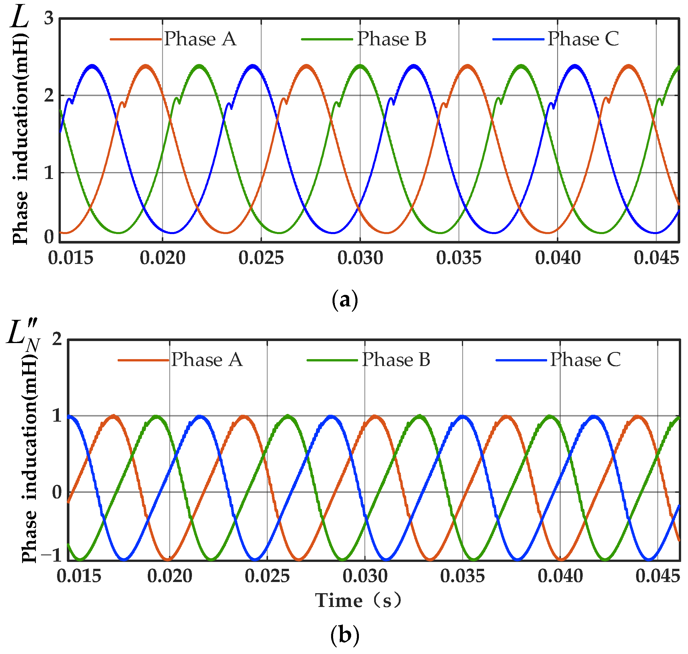
Figure 13.
Comparison of speed estimation results for a given speed of 400 r/min.
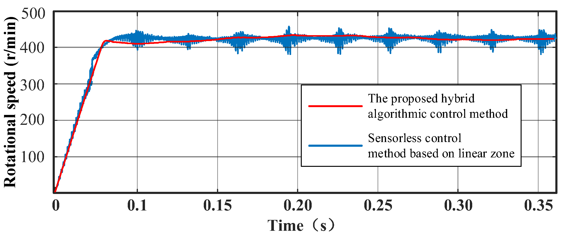
Figure 14.
The simulated waveform of the motor under light load with conventional sensorless control (2 N·m). (a) Three-phase current simulation waveforms; (b) Three-phase inductance simulation waveforms; (c) Comparison of predicted and actual positions; (d) Positional error.
Figure 14.
The simulated waveform of the motor under light load with conventional sensorless control (2 N·m). (a) Three-phase current simulation waveforms; (b) Three-phase inductance simulation waveforms; (c) Comparison of predicted and actual positions; (d) Positional error.
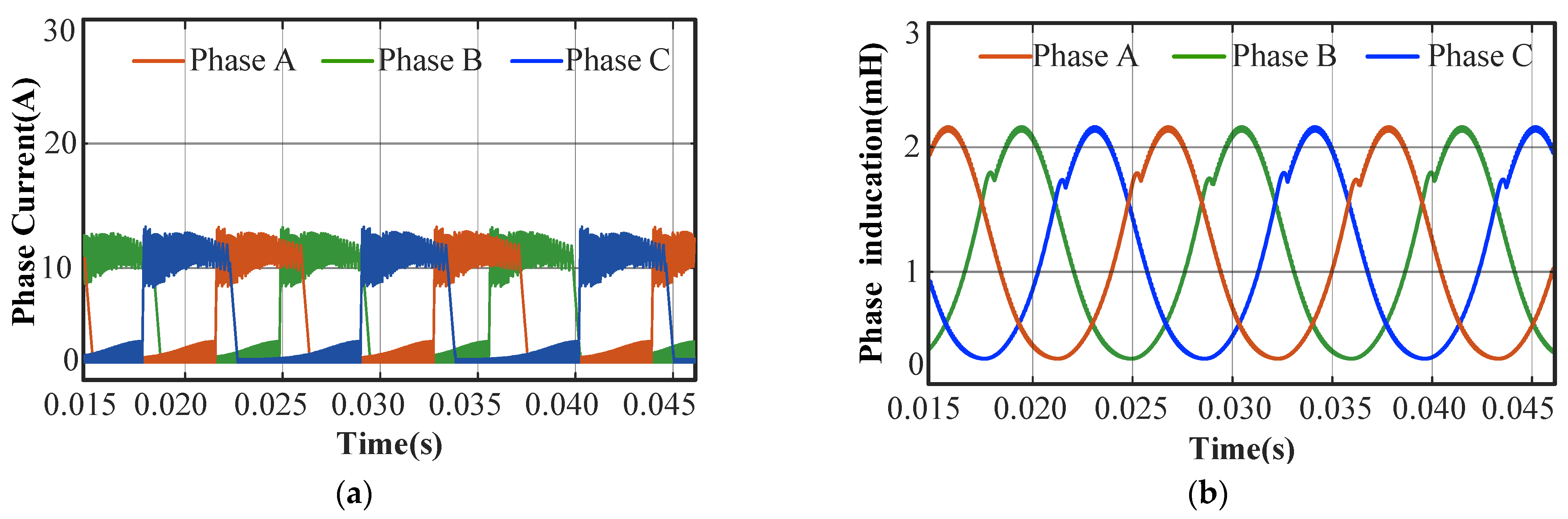
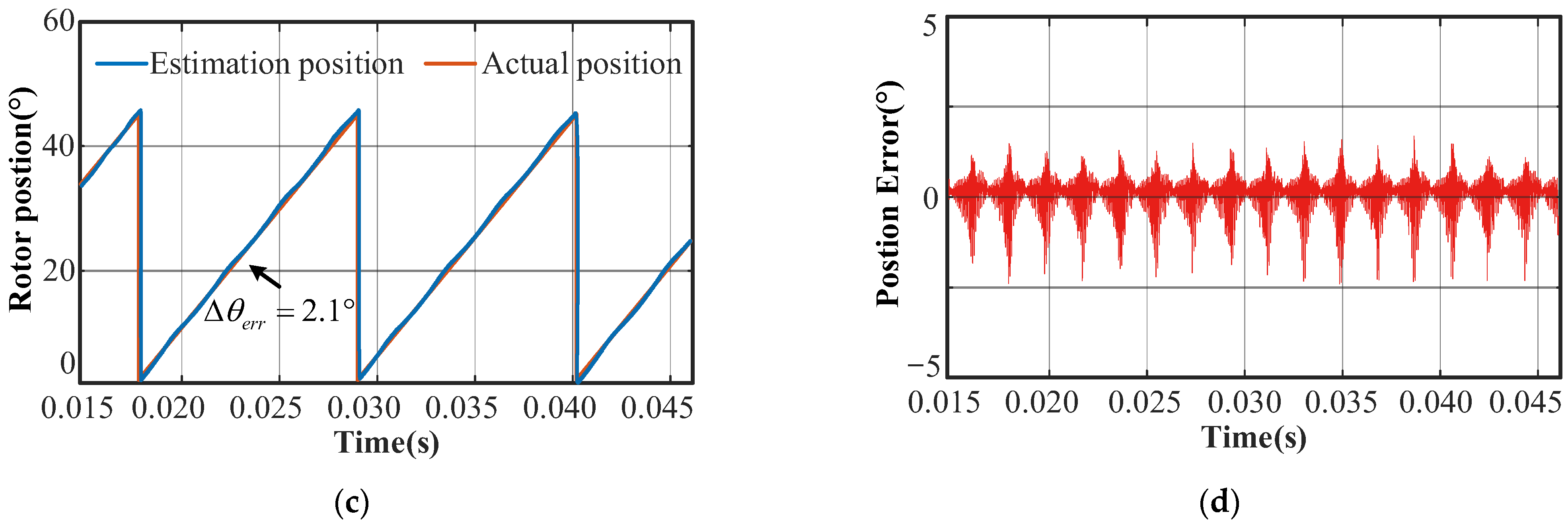
Figure 15.
The simulated waveforms of the motor under light load for the proposed hybrid algorithm (2 N·m); (a) Three-phase current simulation waveforms; (b) Three-phase inductance simulation waveforms; (c) Comparison of predicted and actual positions; (d) Positional error.
Figure 15.
The simulated waveforms of the motor under light load for the proposed hybrid algorithm (2 N·m); (a) Three-phase current simulation waveforms; (b) Three-phase inductance simulation waveforms; (c) Comparison of predicted and actual positions; (d) Positional error.

Figure 16.
The simulated waveform of the motor under full load with conventional sensorless control (5 N·m). (a) Three-phase current simulation waveforms; (b) Three-phase inductance simulation waveforms; (c) Comparison of predicted and actual positions; (d) Positional error.
Figure 16.
The simulated waveform of the motor under full load with conventional sensorless control (5 N·m). (a) Three-phase current simulation waveforms; (b) Three-phase inductance simulation waveforms; (c) Comparison of predicted and actual positions; (d) Positional error.

Figure 17.
The simulated waveforms of the motor under full load for the proposed hybrid algorithm (5 N·m). (a) Three-phase current simulation waveforms; (b) Three-phase inductance simulation waveforms; (c) Comparison of predicted and actual positions; (d) Positional error.
Figure 17.
The simulated waveforms of the motor under full load for the proposed hybrid algorithm (5 N·m). (a) Three-phase current simulation waveforms; (b) Three-phase inductance simulation waveforms; (c) Comparison of predicted and actual positions; (d) Positional error.
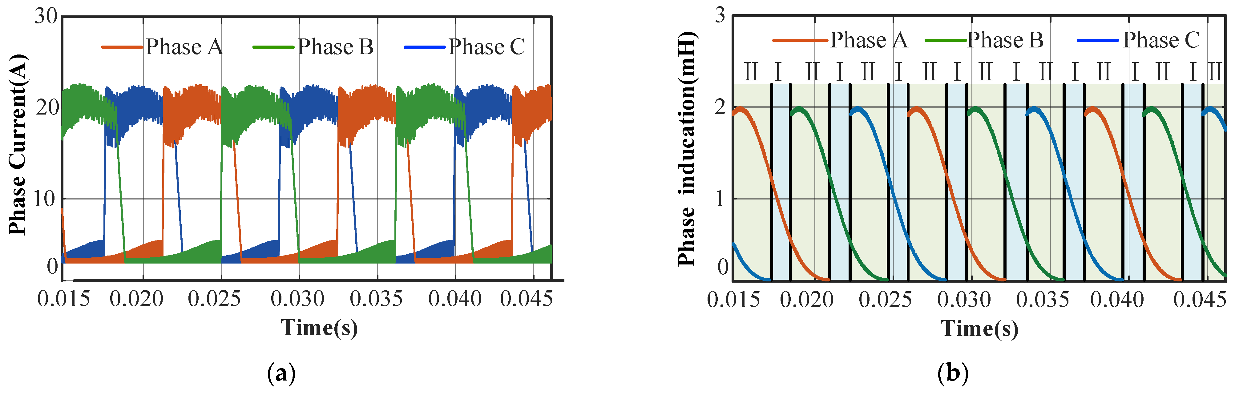

Figure 18.
Sensorless control at 400 r/min under load changes.

Figure 19.
SRM Experimental Platform.
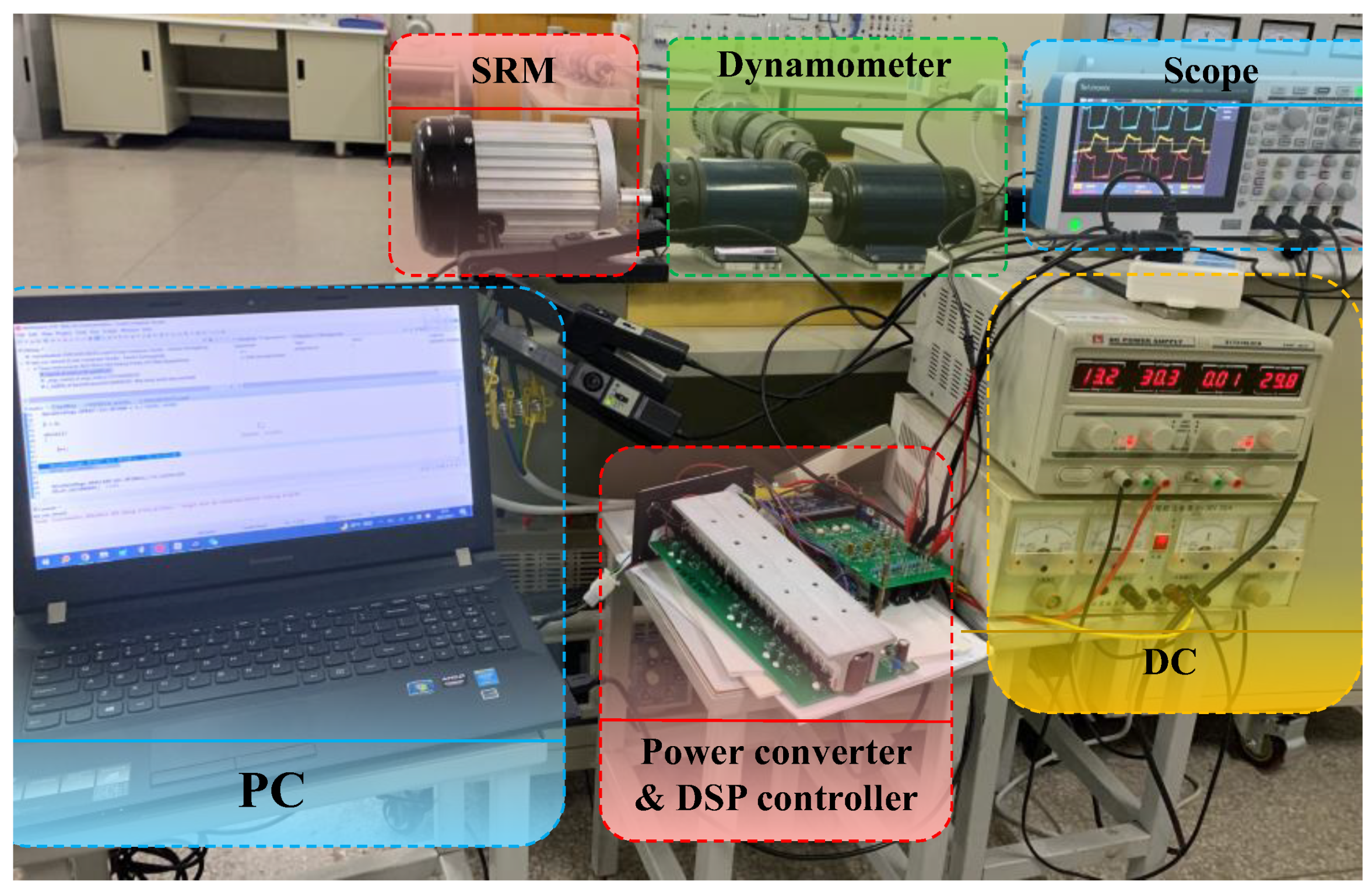
Figure 20.
Phase current and rotor position waveforms at light load (400 r/min and 2 N·m). (a) Waveform of conventional sensorless estimation method; (b) Waveform of sensorless estimation proposed in this paper.
Figure 20.
Phase current and rotor position waveforms at light load (400 r/min and 2 N·m). (a) Waveform of conventional sensorless estimation method; (b) Waveform of sensorless estimation proposed in this paper.

Figure 21.
Phase current and rotor position waveforms at full load (400 r/min and 5 N·m). (a) Waveform of conventional sensorless estimation method; (b) Waveform of sensorless estimation proposed in this paper.
Figure 21.
Phase current and rotor position waveforms at full load (400 r/min and 5 N·m). (a) Waveform of conventional sensorless estimation method; (b) Waveform of sensorless estimation proposed in this paper.

Table 1.
Parameters of the SRM Structure.
| Major Parameters | Values | Major Parameters | Values |
|---|---|---|---|
| Outside diameter of stator | 138 mm | Stator Pole Radian | 17.7° |
| Outer diameter of rotor | 80.7 mm | Rotor Pole Radian | 16.65° |
| The core is stacked long | 97.8 mm | Stator yoke height | 8.8 mm |
| Air gap | 0.35 mm | Rotor yoke height | 7.25 mm |
Table 2.
Main parameters of the SRM system.
| Major Parameters | Values | Major Parameters | Values |
|---|---|---|---|
| Rated Power | 1.5 kW | Rated Load | 5 N·m |
| Bus Voltage | 60 V | Switching Frequency | 10 kHz |
| Rated Speed | 2000 r/min | Given motor speed | 400 r/min |
| Rated Current | 25 A | Median inductance | 1.276 mH |
Table 3.
Summarized position estimation errors in load variation.
| Control Strategy | Simulation Position Estimation Errors | Experiment Position Estimation Errors | ||
|---|---|---|---|---|
| 2 N·m | 5 N·m | 2 N·m | 5 N·m | |
| The linear zone method | 2.1° | 9.3° | 3.6° | 5.8° |
| The proposed methods | 1.3° | 2.7° | 2.5° | 2.7° |
Table 4.
Comparison of the proposed method with the traditional sensorless control methods.
| Control Strategy | Offline Measurements | Computation Burden | Driving with Load | Storage Memory Occupation |
|---|---|---|---|---|
| The linear zone method [30] | Yes | Low | No | Small |
| Intelligent schemes [18,27] | Yes | High | Yes | Large |
| RPLL based method [29] | No | Medium | Yes | Small |
| Unsaturated inductance model based methods [25,26] | Yes | Medium | No | Small |
| Flux-linkage based methods [13] | Yes | Low | Yes | Small |
| The proposed methods | No | Low | Yes | Small |
Disclaimer/Publisher’s Note: The statements, opinions and data contained in all publications are solely those of the individual author(s) and contributor(s) and not of MDPI and/or the editor(s). MDPI and/or the editor(s) disclaim responsibility for any injury to people or property resulting from any ideas, methods, instructions or products referred to in the content. |
© 2023 by the authors. Licensee MDPI, Basel, Switzerland. This article is an open access article distributed under the terms and conditions of the Creative Commons Attribution (CC BY) license (https://creativecommons.org/licenses/by/4.0/).
Share and Cite
MDPI and ACS Style
Ni, F.; Zhang, W.; Bi, Y.; Li, B. The Study of SRM Sensorless Control Strategy Based on SOGI-FLL and ADRC-PLL Hybrid Algorithm. Electronics 2024, 13, 2. https://doi.org/10.3390/electronics13010002
AMA Style
Ni F, Zhang W, Bi Y, Li B. The Study of SRM Sensorless Control Strategy Based on SOGI-FLL and ADRC-PLL Hybrid Algorithm. Electronics. 2024; 13(1):2. https://doi.org/10.3390/electronics13010002
Chicago/Turabian StyleNi, Fuyin, Wenchao Zhang, Yuchun Bi, and Bo Li. 2024. "The Study of SRM Sensorless Control Strategy Based on SOGI-FLL and ADRC-PLL Hybrid Algorithm" Electronics 13, no. 1: 2. https://doi.org/10.3390/electronics13010002
Note that from the first issue of 2016, this journal uses article numbers instead of page numbers. See further details here.