
A 1 + α Order Generalized Butterworth Filter Structure and Its Field Programmable Analog Array Implementation


1
Electronics Laboratory, Department of Physics, University of Patras, GR-26504 Rio Patras, Greece
2
Department of Electrical and Computer Engineering, University of Sharjah, Sharjah P.O. Box 27272, United Arab Emirates
3
Nanoelectronics Integrated Systems Center (NISC), Nile University, Giza 12677, Egypt
4
Department of Electrical and Software Engineering, University of Calgary, Calgary, AB T2N 1N4, Canada
*
Author to whom correspondence should be addressed.
Electronics 2023, 12(5), 1225; https://doi.org/10.3390/electronics12051225
Submission received: 30 January 2023
/
Revised: 22 February 2023
/
Accepted: 27 February 2023
/
Published: 3 March 2023
(This article belongs to the Special Issue Embedded and Integrated Circuits and Systems in Real Engineering Applications)
Abstract
:Fractional-order Butterworth filters of order 1 + (0 < < 1) can be implemented by a unified structure, using the method presented in this paper. The main offered benefit is that the cutoff frequencies of the filters are fully controllable using a very simple method and, also, various types of filters (e.g., low-pass, high-pass, band-pass, and band-stop) could be realized. Thanks to the employment of a Field Programmable Analog Array device, the implementation of the introduced method is fully reconfigurable, in the sense that various types of filter functions as well as their order are both programmable.
1. Introduction
Fractional-order filters offer a fine adjustment of the slope of the attenuation from the pass-band to the stop-band, and this is the result of the fact that it is equal to dB/dec, where n is the integer part of the order and 0 < < 1 is its non-integer counterpart [1,2,3,4]. In addition, they offer the scaling of the cutoff frequencies due to their dependence on both the pole frequency and the order of the filter. In the case of filters of order 0 < < 1, there are simple expressions describing the dependence of the cutoff frequencies on the aforementioned parameters. This is not the case for filters with the order 1 + , where complicated non-linear equations must be solved to find the value of the cutoff frequency. In addition, the realization of well-known filter functions such as the Butterworth transfer functions is an even more difficult task [5,6].
A significant research effort has been dedicated to overcoming this obstacle, where appropriate cost functions error minimization metaheuristic and genetic algorithms were reported. A first attempt for approximating fractional-order Butterworth filters has been performed in [7], where a polynomial fitting-based method was used for expressing the coefficients of the fractional-order transfer function as a function of the order of the filter. This method is oriented to the realization of low-pass filters, and the high-pass filter functions have been derived through a frequency transformation. In [8], the approximation of the fractional-order Butterworth low-pass filters is performed using the pole placement in the W-plane. In [9], the Flower Pollination Algorithm (FPA) with an appropriate cost function is employed for approximating Butterworth low-pass filters, while in [10], a nature-inspired optimization technique called the Gravitational Search Algorithm (GSA) has been employed for the same purpose. In [11], the Symbiotic Organisms Search (SOS) algorithm is presented for approximating Butterworth high-pass filters. In [12], a genetic algorithm is introduced for approximating Butterworth low-pass filters.
From the above, it is readily obtained that the solutions which are available in the literature are based on the employment of relatively complicated optimization algorithms. In addition, they do not offer a simultaneous approximation of different types of Butterworth filter functions, such as the low-pass, high-pass, band-pass, and band-stop.
In the present work, a simple procedure for realizing various types of 1 + order Butterworth transfer functions, with fully controllable cutoff frequencies, is introduced. It is based on the fit of the frequency response magnitude data by a minimum-phase state-space model, using a Log-Chebyshev magnitude design. The main important benefits are as follows: (a) The procedure is independent of the type of the filter; low-pass, high-pass, band-pass, and band-stop filter functions can be implemented. (b) The resulting structure has the capability of implementing all the aforementioned filter functions without altering its core.
This paper is organized as follows: The description of the basic characteristics of the fractional filters of order 1 + is performed in Section 2. The proposed procedure is introduced in Section 3, where a possible implementation of the resulting approximation functions using a Field Programmable Array (FPAA) device is also demonstrated. The performance of the designed filters is experimentally verified in Section 4.
2. Fractional-Order Filters of Order 1 + (0 < < 1)
Let us consider the transfer function of a low-pass filter of order and pole frequency , with the variable being a time constant
Setting in (1), the following expression of the magnitude response is derived:
The cutoff or half-power frequency of the filter (), defined as the frequency where there is a 3 dB drop in the magnitude from its maximum value, is determined using (2) and setting . The resulting expression is given by (3)
In a similar way, the behavior of a high-pass filter is described by (4) and (5) and the associated cutoff frequency is given by the expression in (6)
Inspecting (3) and (6), it is readily obtained that, having available the pole frequency and the order of the filter, the cutoff frequency can be fully determined.
In the case of a 1 + order low-pass filter, its transfer function is given by (7)
with Q being a factor equal to the quality factor of the corresponding second-order filter. The half-power frequency is the solution of the following non-linear equation:
The corresponding non-linear equation for obtaining the half-power frequency of a high-pass filter, described by (9),
is provided by (10)
The peak (center) frequency is calculated by solving the differential equation:
, while the associated lower () and upper () cutoff frequencies are calculated by setting .
From the above, it is clear that the determination of the characteristic frequencies in the case of 1 + order filters is a difficult procedure, which is the reason for using the aforementioned algorithmic methods. This obstacle can be overcome through the utilization of the curve fitting-based procedure which will be described in the next section.
3. Proposed Procedure for Approximating 1 + Order Filters
3.1. Derivation of the Rational Integer-Order Approximation Function
According to the proposed method, the starting point is the consideration of the gain responses of the filters. For example, the corresponding expressions of low-pass, high-pass, band-pass, and band-stop Butterworth-type filters are those in (13)–(16).
The next step is to collect the values of the gain of the filter transfer function of interest within the desired range (). This can be performed through the utilization of the MATLAB frd built-in function. The last steps include the fit of the collected gain data with a minimum-phase state-space model using the Log-Chebyshev magnitude design, realized using the MATLAB built-in command fitmagfrd, and the derivation of the corresponding rational integer-order transfer function using the tf MATLAB command.
The resulting transfer function will have the form of (17)
with and being positive and real coefficients, and n being the order of the approximation.
Considering Butterworth low-pass and high-pass filters of order 1.2, 1.4, and 1.6, with cutoff frequency =1 rad/s and approximated by a 4th-order approximation within the range of [10, 101] rad/s, the resulting values of the coefficients and are summarized in Table 1 and Table 2. In the case of a band-pass filter, the same order of approximation is considered. While the peak and cutoff frequencies are = 1 rad/s, = 0.5 rad/s, and = 2 rad/s, for the band-stop filter, the corresponding values are = 1 rad/s, = 0.2 rad/s, and = 5 rad/s. The values of the coefficients are provided in Table 3 and Table 4.
3.2. A Possible Implementation
A possible realization of the transfer function in (17) is using the Follow-the-Leader Feedback (FLF) structure in Figure 3, where the realized transfer function is given by (18) [13].
The implementation of the integration blocks in Figure 3 can be performed using a variety of active blocks, including Operational Amplifiers (op-amps), Second-Generation Current Conveyors (CCIIs), and Current Feedback Operational Amplifiers (CFOAs). The derived implementations are active-RC structures which do not offer the electronic tunability of the characteristics of the filters. The employment of the Operational Transconductance Amplifiers (OTAs) as active elements is a solution for overcoming this obstacle due to the fact that the transconductance parameter of the OTA can be electronically adjusted by an appropriate dc current/voltage. The price paid for this achievement is the reduced linearity of the resulting filter structures, and this is caused by the small-signal nature of the transconductance [14]. Another option could be the utilization of a digitally programmable device [15], such as the FPAA AN231E04 device provided by Anadigm [16].
Denormalizing (17) at = 150 krad/s and taking into account that the integration constants () of the FPAA device are formed as (), (having units of s), their values are summarized in Table 5, Table 6, Table 7 and Table 8, where the values of the scaling factors (j = 0 ...4) are also given. The clock frequency is equal to = 2 MHz. In addition, according to the specifications of the FPAA, the realizable values of the integration constants are in the range [0.02, 17.7] s, while the weight factors of the summation stages for realizing the scaling factors are in the range [0.01, 8.83]. Inspecting Table 5, Table 6, Table 7 and Table 8, it is derived that there are values of and that are not realizable. As the range of the realizable values of the gain stages is [0.01, 100], the problem can be solved by following the technique presented in Figure 4. According to this, the desired value of the gain scaling factor is implemented as , making the values of to be in the realizable range. In the FPAA implementation presented in the next section, this will be performed by adding an extra gain stage to each one of the inputs of the summation stages, and both of them will have a value equal to , establishing a total gain equal to in the path of the associated signal. A similar approach will be followed for the integration constants.
4. Experimental Results
Using the Anadigm Designer® 2 EDA software, the resulting design is depicted in Figure 5, while the experimental setup is demonstrated in Figure 6a. The FPAA device with the accompanied printed circuit board (PCB) for implementing the required single-to-differential and differential-to-single voltage conversion is demonstrated in Figure 6b. The corresponding circuitry of the interface for performing a single-to-differential conversion of the input signal is depicted in Figure 7a, where the corresponding one for performing the differential-to-single conversion of the output signal is demonstrated in Figure 7b. Taking into account the terminal properties of the CFOA, described by the following formulas, , the expressions in (20) and (21) are readily obtained for the topology in Figure 7a.
The value of the dc voltage source is E = 3 V, and this is originated from the fact that the common-mode voltage of the FPAA is equal to 1.5 V.
The topology in Figure 7b implements the following input–output relationship
The and are given by the formulas and . The AD844 discrete component is chosen for implementing the required CFOAs [17] while the value of the basic resistor is R = 10 k.
The frequency responses of the Butterworth low-pass and high-pass filters, which are obtained using the HP4395A Network/Impedance analyzer, are demonstrated in Figure 8a,b, respectively. The measured values of the cutoff frequencies were 151.1 rad/s for the low-pass filter and 147.8 rad/s for the high-pass filter, close to the theoretical value of 150 krad/s. The experimental results of the band-pass and band-stop filters are provided in Figure 9a,b. The measured value of the lower cutoff frequency of the band-pass filters was 74.7 krad/s, with the theoretical value being 75 krad/s. The corresponding values of the band-stop filters were 11.8 krad/s and 298.1 krad/s, with the associated theoretical values being 12 krad/s and 300 krad/s, respectively.
These slight deviations from the theory are mainly caused by the tolerances of the resistors employed in the interfacing stages as well as by the truncation of the values of the time constants and the scaling factors performed by the FPAA device.
The time-domain behavior of the filters has been evaluated by stimulating the low-pass and high-pass filters (order equal to 1.4) by a 1Vp-p sinusoidal signal with a frequency equal to their cutoff frequency. The waveforms, obtained using a DSO6034A digital oscilloscope, are demonstrated in Figure 10a,b. The values of the corresponding gains were −3.06 dB and −3.4 dB, confirming their time-domain performance. In the case of the band-pass filters, the stimulation of a filter of an order equal to 1.4 by sinusoidal inputs of the same amplitude as in the previous case and of a frequency equal to the peak frequency results in the waveforms in Figure 10c, where the expected gain of 0 dB is confirmed.
5. Conclusions
A versatile procedure for approximating various types of Butterworth filters with fully controllable frequency characteristics is introduced in this work. The algorithm is based on the built-in commands frd, fitmagfrd, and tf of the MATLAB software, leading to a rational integer-order transfer function. This can be implemented using the well-known classical filter design techniques, such as multi-feedback or cascaded structures. The choice of the technique, as well as of the utilized active element, is up to the designer, performing a trade-off between the design complexity and electronic tunability.
The experimental results derived using an FPAA device confirm the validity of the proposed concept. Future research steps include the application of the presented concept for implementing other types of filter functions, such as Chebyshev filters [18,19,20,21], Bessel filters [22,23,24], and elliptic filters [25].
Author Contributions
Conceptualization, C.P., J.N. and A.S.E.; methodology, J.N. and C.P.; software, J.N.; validation, J.N; formal analysis, J.N.; investigation, J.N. and C.P.; writing—original draft preparation, C.P.; writing—review and editing, C.P. and A.S.E.; project administration, C.P. and A.S.E. All authors have read and agreed to the published version of the manuscript.
Funding
This research received no external funding.
Institutional Review Board Statement
Not applicable.
Informed Consent Statement
Not applicable.
Data Availability Statement
No new data were created or analyzed in this study. Data sharing is not applicable to this article.
Conflicts of Interest
The authors declare no conflict of interest.
Abbreviations
The following abbreviations are used in this manuscript:
| AMS | Austria Mikro Systeme |
| CCII | Second-Generation Current Conveyor |
| CFOA | Current Feedback Operational Amplifier |
| CMOS | Complimentary Metal-Oxide Semiconductor |
| EDA | Electronic Design Automation |
| FLF | Follow-the-Leader Feedback |
| FPA | Flower Pollination Algorithm |
| FPAA | Field Programmable Analog Array |
| GSA | Gravitational Search Algorithm |
| MOS | Metal-Oxide Semiconductor |
| OP-AMP | Operational Amplifier |
| OTA | Operational Transconductance Amplifier |
| PCB | Printed Circuit Board |
| RC | Resistor Capacitor |
| SOS | Symbiotic Organisms Search |
References
- Bertsias, P.; Khateb, F.; Kubanek, D.; Khanday, F.A.; Psychalinos, C. Capacitorless digitally programmable fractional-order filters. AEU-Int. J. Electron. Commun. 2017, 78, 228–237. [Google Scholar] [CrossRef]
- Jerabek, J.; Sotner, R.; Dvorak, J.; Polak, J.; Kubanek, D.; Herencsar, N.; Koton, J. Reconfigurable fractional-order filter with electronically controllable slope of attenuation, pole frequency and type of approximation. J. Circuits Syst. Comput. 2017, 26, 1750157. [Google Scholar] [CrossRef] [Green Version]
- Dvorak, J.; Langhammer, L.; Jerabek, J.; Koton, J.; Sotner, R.; Polak, J. Synthesis and analysis of electronically adjustable fractional-order low-pass filter. J. Circuits Syst. Comput. 2018, 27, 1850032. [Google Scholar] [CrossRef]
- Langhammer, L.; Dvorak, J.; Sotner, R.; Jerabek, J.; Bertsias, P. Reconnection–Less reconfigurable low–Pass filtering topology suitable for higher–Order fractional–Order design. J. Adv. Res. 2020, 25, 257–274. [Google Scholar] [CrossRef] [PubMed]
- Freeborn, T.J. Comparison of (1 + α) Fractional-Order Transfer Functions to Approximate Lowpass Butterworth Magnitude Responses. Circuits, Syst. Signal Process. 2016, 35, 1983–2002. [Google Scholar] [CrossRef]
- Tsirimokou, G.; Psychalinos, C.; Elwakil, A. Design of CMOS Analog Integrated Fractional-Order Circuits: Applications in Medicine and Biology; Springer: Berlin/Heidelberg, Germany, 2017. [Google Scholar]
- Freeborn, T.J.; Maundy, B.; Elwakil, A.S. Field programmable analogue array implementation of fractional step filters. IET Circ. Devices Syst. 2010, 4, 514–524. [Google Scholar] [CrossRef]
- Mishra, S.K.; Upadhyay, D.K.; Gupta, M. Approximation of Fractional-Order Butterworth Filter Using Pole-Placement in W-Plane. IEEE Trans. Circ. Syst. II Express Briefs 2021, 68, 3229–3233. [Google Scholar] [CrossRef]
- Mahata, S.; Kar, R.; Mandal, D. Optimal design of fractional-order Butterworth filter with improved accuracy and stability margin. In Fractional-Order Modeling of Dynamic Systems with Applications in Optimization, Signal Processing and Control; Elsevier: Amsterdam, The Netherlands, 2022; pp. 293–321. [Google Scholar]
- Mahata, S.; Saha, S.K.; Kar, R.; Mandal, D. Optimal design of fractional order low pass Butterworth filter with accurate magnitude response. Digit. Signal Process. 2018, 72, 96–114. [Google Scholar] [CrossRef]
- Mahata, S.; Kar, R.; Mandal, D. Optimal fractional-order highpass Butterworth magnitude characteristics realization using current-mode filter. AEU-Int. J. Electron. Commun. 2019, 102, 78–89. [Google Scholar] [CrossRef]
- Mahata, S.; Banerjee, S.; Kar, R.; Mandal, D. Revisiting the use of squared magnitude function for the optimal approximation of (1 + α)-order Butterworth filter. AEU-Int. J. Electron. Commun. 2019, 110, 152826. [Google Scholar] [CrossRef]
- Tsirimokou, G.; Psychalinos, C.; Elwakil, A.S.; Salama, K.N. Electronically tunable fully integrated fractional-order resonator. IEEE Trans. Circ. Syst. II Express Briefs 2017, 65, 166–170. [Google Scholar] [CrossRef] [Green Version]
- Tsirimokou, G.; Psychalinos, C.; Elwakil, A.S. Fractional-order electronically controlled generalized filters. Int. J. Circuit Theory Appl. 2017, 45, 595–612. [Google Scholar] [CrossRef]
- Tlelo-Cuautle, E.; Pano-Azucena, A.D.; Guillén-Fernández, O.; Silva-Juárez, A. Analog/Digital Implementation of Fractional Order Chaotic Circuits and Applications; Springer: Berlin/Heidelberg, Germany, 2020. [Google Scholar]
- Anadigm. AN231E04 dpASP: The AN231E04 dpASP Dynamically Reconfigurable Analog Signal Processor. Available online: https://anadigm.com/an231e04.asp (accessed on 3 January 2023).
- Devices, A. MHz 2000 V/μs Monolithic Op Amp with Quad Low Noise AD844 Data Sheet, Revision G; One Technology Way: Noorwood, MA, USA, 2009; p. 60. [Google Scholar]
- Freeborn, T.; Maundy, B.; Elwakil, A.S. Approximated fractional order Chebyshev lowpass filters. Math. Probl. Eng. 2015, 2015, 832468. [Google Scholar] [CrossRef]
- Freeborn, T.J.; Elwakil, A.S.; Maundy, B. Approximated fractional-order inverse Chebyshev lowpass filters. Circuits Syst. Signal Process. 2016, 35, 1973–1982. [Google Scholar] [CrossRef]
- AbdelAty, A.M.; Soltan, A.; Ahmed, W.A.; Radwan, A.G. Fractional order Chebyshev-like low-pass filters based on integer order poles. Microelectron. J. 2019, 90, 72–81. [Google Scholar] [CrossRef]
- Daryani, R.; Aggarwal, B.; Gupta, M. Design of Fractional-Order Chebyshev Low-Pass Filter for Optimized Magnitude Response Using Metaheuristic Evolutionary Algorithms. Circuits Syst. Signal Process. 2022, 1–31. [Google Scholar] [CrossRef]
- Ćoza, A.; Županović, V.; Vlah, D.; Jurišić, D. Group delay of fractional n+ α-order Bessel filters. In Proceedings of the IEEE 2020 43rd International Convention on Information, Communication and Electronic Technology (MIPRO), Opatija, Croatia, 28 September–2 October 2020; pp. 163–168. [Google Scholar]
- Soni, A.; Gupta, M. Analysis and design of optimized fractional order low-pass Bessel filter. J. Circuits Syst. Comput. 2021, 30, 2150035. [Google Scholar] [CrossRef]
- Soni, A.; Gupta, M. Designing of Fractional Order Bessel Filter using Optimization Techniques. Int. J. Electron. Lett. 2022, 10, 71–86. [Google Scholar] [CrossRef]
- Kubanek, D.; Freeborn, T.J.; Koton, J.; Dvorak, J. Validation of fractional-order lowpass elliptic responses of (1 + α)-order analog filters. Appl. Sci. 2018, 8, 2603. [Google Scholar] [CrossRef] [Green Version]
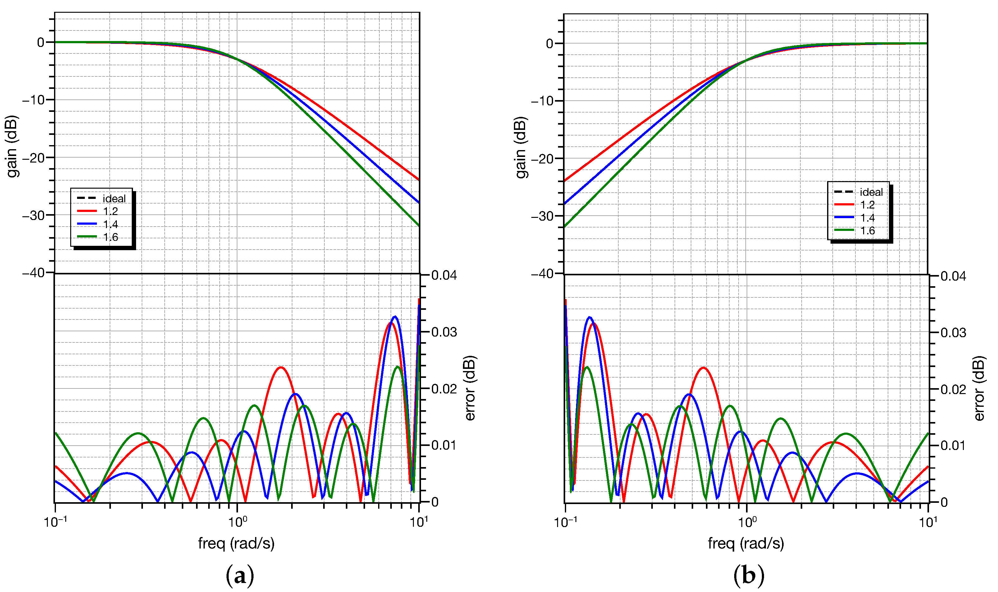
Figure 1.
Frequency responses of the approximated Butterworth (a) low-pass filters and (b) high-pass filters of orders 1.2, 1.4, and 1.6.
Figure 1.
Frequency responses of the approximated Butterworth (a) low-pass filters and (b) high-pass filters of orders 1.2, 1.4, and 1.6.

Figure 2.
Frequency responses of the approximated Butterworth (a) band-pass filters and (b) band-stop filters of orders 1.2, 1.4, and 1.6.
Figure 2.
Frequency responses of the approximated Butterworth (a) band-pass filters and (b) band-stop filters of orders 1.2, 1.4, and 1.6.

Figure 3.
Follow-the-Leader Feedback block diagram for implementing the transfer function in (17).
Figure 3.
Follow-the-Leader Feedback block diagram for implementing the transfer function in (17).

Figure 4.
Concept for enhancing the range of the implementable scaling factors.

Figure 5.
FPAA configuration for realizing Butterworth low-pass, high-pass, band-pass, and band-stop filters.
Figure 5.
FPAA configuration for realizing Butterworth low-pass, high-pass, band-pass, and band-stop filters.

Figure 6.
(a) Experimental setup for evaluating the performance of the implemented filters, (b) FPAA device along with the associated interface.
Figure 6.
(a) Experimental setup for evaluating the performance of the implemented filters, (b) FPAA device along with the associated interface.

Figure 7.
Circuitry for performing (a) single-to-differential conversion of the input signal and (b) circuitry for performing differential-to-single conversion of the output signal.
Figure 7.
Circuitry for performing (a) single-to-differential conversion of the input signal and (b) circuitry for performing differential-to-single conversion of the output signal.

Figure 8.
Experimental frequency responses of the Butterworth (a) low-pass filters and (b) high-pass filters of orders 1.2, 1.4, 1.6, realized using the FPAA configuration in Figure 5.
Figure 8.
Experimental frequency responses of the Butterworth (a) low-pass filters and (b) high-pass filters of orders 1.2, 1.4, 1.6, realized using the FPAA configuration in Figure 5.
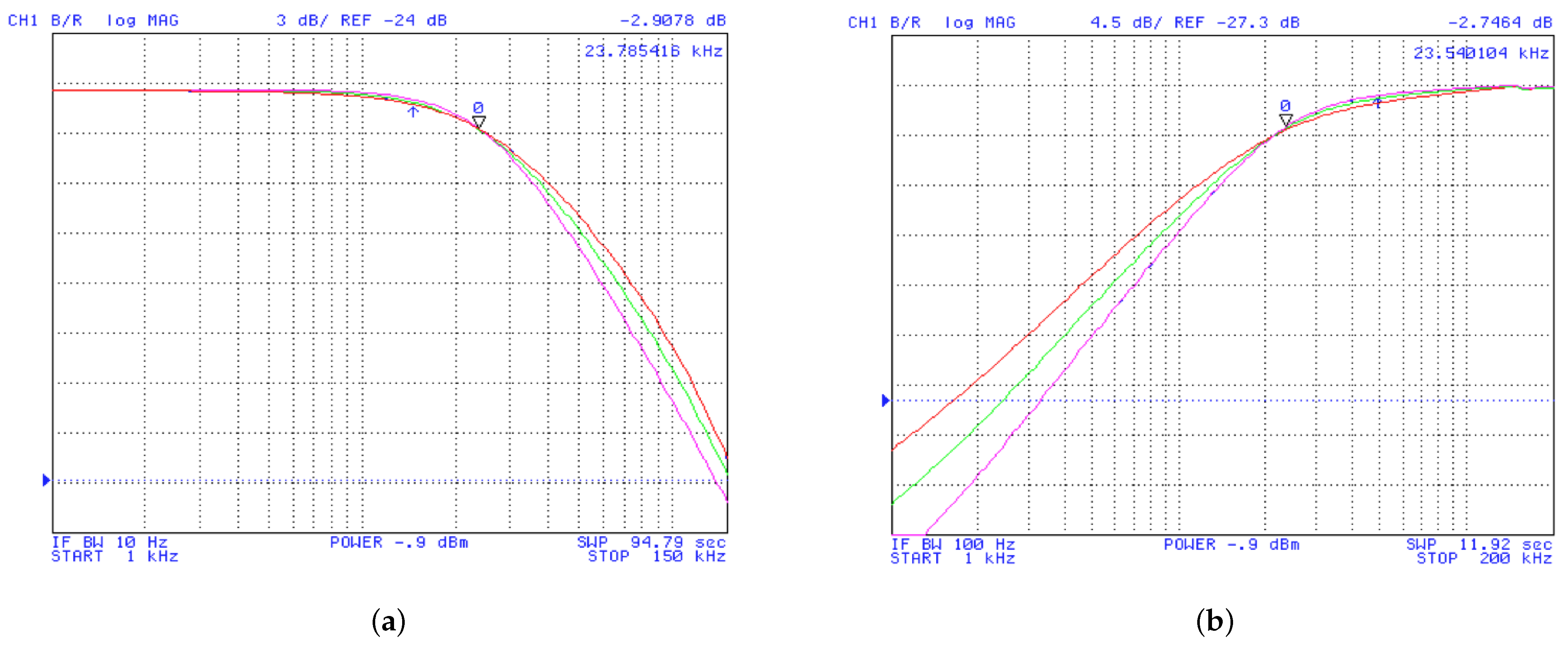
Figure 9.
Experimental frequency responses of the Butterworth (a) band-pass filters and (b) band-stop filters of orders 1.2, 1.4, 1.6, realized using the FPAA configuration in Figure 5.
Figure 9.
Experimental frequency responses of the Butterworth (a) band-pass filters and (b) band-stop filters of orders 1.2, 1.4, 1.6, realized using the FPAA configuration in Figure 5.

Figure 10.
Experimental input and output waveforms of (a) low-pass filter, (b) high-pass filter, and (c) band-pass filter of order equal to 1.4.
Figure 10.
Experimental input and output waveforms of (a) low-pass filter, (b) high-pass filter, and (c) band-pass filter of order equal to 1.4.


Table 1.
Values of coefficients for approximating Butterworth low-pass filters of order 1.2, 1.4, 1.6 ( = 1 rad/s).
Table 1.
Values of coefficients for approximating Butterworth low-pass filters of order 1.2, 1.4, 1.6 ( = 1 rad/s).
| Coefficient | Order | ||
|---|---|---|---|
| 1.2 | 1.4 | 1.6 | |
| 0.005867 | 0.00228 | 0.001421 | |
| 0.6167 | 0.3336 | 0.1768 | |
| 5.149 | 3.841 | 2.674 | |
| 6.85 | 6.96 | 6.071 | |
| 1.704 | 1.769 | 1.64 | |
| 7.196 | 7.014 | 6.537 | |
| 12.66 | 12.4 | 10.97 | |
| 8.606 | 8.877 | 7.976 | |
| 1.701 | 1.77 | 1.644 |
Table 2.
Values of coefficients for approximating Butterworth high-pass filters of order 1.2, 1.4, 1.6 ( = 1 rad/s).
Table 2.
Values of coefficients for approximating Butterworth high-pass filters of order 1.2, 1.4, 1.6 ( = 1 rad/s).
| Coefficient | Order | ||
|---|---|---|---|
| 1.2 | 1.4 | 1.6 | |
| 1.002 | 0.9991 | 0.9974 | |
| 4.028 | 3.932 | 3.693 | |
| 3.028 | 2.17 | 1.627 | |
| 0.3626 | 0.1884 | 0.1075 | |
| 0.00345 | 0.001288 | 0.0008641 | |
| 5.06 | 5.015 | 4.852 | |
| 7.446 | 7.003 | 6.676 | |
| 4.231 | 3.962 | 3.976 | |
| 0.588 | 0.565 | 0.6083 |
Table 3.
Values of coefficients for approximating Butterworth band-pass filters of order 1.2, 1.4, 1.6 ( = 1 rad/s, = 0.5 rad/s, = 2 rad/s).
Table 3.
Values of coefficients for approximating Butterworth band-pass filters of order 1.2, 1.4, 1.6 ( = 1 rad/s, = 0.5 rad/s, = 2 rad/s).
| Coefficient | Order | ||
|---|---|---|---|
| 1.2 | 1.4 | 1.6 | |
| 0.002795 | 0.002358 | 0.004134 | |
| 0.9857 | 0.632 | 0.4071 | |
| 4.828 | 4.016 | 3.325 | |
| 0.9857 | 0.632 | 0.4071 | |
| 0.002795 | 0.002358 | 0.004134 | |
| 4.448 | 3.73 | 3.118 | |
| 6.772 | 5.939 | 5.246 | |
| 4.448 | 3.73 | 3.118 | |
| 1 | 1 | 1 |
Table 4.
Values of coefficients for approximating Butterworth band-stop filters of order 1.2, 1.4, 1.6 ( = 1 rad/s, = 0.2 rad/s, = 5 rad/s).
Table 4.
Values of coefficients for approximating Butterworth band-stop filters of order 1.2, 1.4, 1.6 ( = 1 rad/s, = 0.2 rad/s, = 5 rad/s).
| Coefficient | Order | ||
|---|---|---|---|
| 1.2 | 1.4 | 1.6 | |
| 1.271 | 1.815 | 2.373 | |
| 0.1948 | 0.1959 | 0.1668 | |
| 2.542 | 3.63 | 4.747 | |
| 0.1948 | 0.1959 | 0.1668 | |
| 1.271 | 1.815 | 2.373 | |
| 8.074 | 13.59 | 18.94 | |
| 4.52 | 8.957 | 19.05 | |
| 8.074 | 13.59 | 18.94 | |
| 1 | 1 | 1 |
Table 5.
Values of the integration constants and scaling factors of the FPAA device for approximating Butterworth low-pass filters of order 1.2, 1.4, 1.6 ( = 150 krad/s).
Table 5.
Values of the integration constants and scaling factors of the FPAA device for approximating Butterworth low-pass filters of order 1.2, 1.4, 1.6 ( = 150 krad/s).
| Coefficient | Order | ||
|---|---|---|---|
| 1.2 | 1.4 | 1.6 | |
| 1.079 | 1.052 | 0.980 | |
| 0.264 | 0.265 | 0.252 | |
| 0.102 | 0.107 | 0.109 | |
| 0.030 | 0.030 | 0.031 | |
| 1.002 | 0.999 | 0.997 | |
| 0.796 | 0.784 | 0.761 | |
| 0.401 | 0.310 | 0.244 | |
| 0.086 | 0.048 | 0.027 | |
| 0.006 | 0.002 | 0.001 |
Table 6.
Values of the integration constants and scaling factors of the FPAA device for approximating Butterworth high-pass filters of order 1.2, 1.4, 1.6 ( = 150 krad/s).
Table 6.
Values of the integration constants and scaling factors of the FPAA device for approximating Butterworth high-pass filters of order 1.2, 1.4, 1.6 ( = 150 krad/s).
| Coefficient | Order | ||
|---|---|---|---|
| 1.2 | 1.4 | 1.6 | |
| 0.759 | 0.752 | 0.728 | |
| 0.220 | 0.209 | 0.206 | |
| 0.085 | 0.085 | 0.089 | |
| 0.021 | 0.021 | 0.023 | |
| 0.006 | 0.002 | 0.001 | |
| 0.086 | 0.047 | 0.027 | |
| 0.407 | 0.310 | 0.244 | |
| 0.796 | 0.784 | 0.761 | |
| 1.002 | 0.999 | 0.997 |
Table 7.
Values of the integration constants and scaling factors of the FPAA device for approximating Butterworth band-pass filters of order 1.2, 1.4, 1.6 ( = 150 krad/s, = 75 krad/s, = 300 krad/s).
Table 7.
Values of the integration constants and scaling factors of the FPAA device for approximating Butterworth band-pass filters of order 1.2, 1.4, 1.6 ( = 150 krad/s, = 75 krad/s, = 300 krad/s).
| Coefficient | Order | ||
|---|---|---|---|
| 1.2 | 1.4 | 1.6 | |
| 0.667 | 0.559 | 0.468 | |
| 0.228 | 0.239 | 0.252 | |
| 0.098 | 0.094 | 0.089 | |
| 0.034 | 0.040 | 0.048 | |
| 0.003 | 0.002 | 0.004 | |
| 0.221 | 0.169 | 0.131 | |
| 0.713 | 0.676 | 0.634 | |
| 0.223 | 0.169 | 0.131 | |
| 0.003 | 0.002 | 0.004 |
Table 8.
Values of the integration constants and scaling factors of the FPAA device for approximating Butterworth band-stop filters of order 1.2, 1.4, 1.6 ( = 60 krad/s, = 12 krad/s, = 300 krad/s).
Table 8.
Values of the integration constants and scaling factors of the FPAA device for approximating Butterworth band-stop filters of order 1.2, 1.4, 1.6 ( = 60 krad/s, = 12 krad/s, = 300 krad/s).
| Coefficient | Order | ||
|---|---|---|---|
| 1.2 | 1.4 | 1.6 | |
| 0.484 | 0.816 | 1.1362 | |
| 0.033 | 0.039 | 0.060 | |
| 0.207 | 0.092 | 0.060 | |
| 0.007 | 0.004 | 0.003 | |
| 1.271 | 1.815 | 2.373 | |
| 0.024 | 0.014 | 0.009 | |
| 0.562 | 0.405 | 0.2492 | |
| 0.024 | 0.014 | 0.009 | |
| 1.271 | 1.815 | 2.373 |
Disclaimer/Publisher’s Note: The statements, opinions and data contained in all publications are solely those of the individual author(s) and contributor(s) and not of MDPI and/or the editor(s). MDPI and/or the editor(s) disclaim responsibility for any injury to people or property resulting from any ideas, methods, instructions or products referred to in the content. |
© 2023 by the authors. Licensee MDPI, Basel, Switzerland. This article is an open access article distributed under the terms and conditions of the Creative Commons Attribution (CC BY) license (https://creativecommons.org/licenses/by/4.0/).
Share and Cite
MDPI and ACS Style
Nako, J.; Psychalinos, C.; Elwakil, A.S. A 1 + α Order Generalized Butterworth Filter Structure and Its Field Programmable Analog Array Implementation. Electronics 2023, 12, 1225. https://doi.org/10.3390/electronics12051225
AMA Style
Nako J, Psychalinos C, Elwakil AS. A 1 + α Order Generalized Butterworth Filter Structure and Its Field Programmable Analog Array Implementation. Electronics. 2023; 12(5):1225. https://doi.org/10.3390/electronics12051225
Chicago/Turabian StyleNako, Julia, Costas Psychalinos, and Ahmed S. Elwakil. 2023. "A 1 + α Order Generalized Butterworth Filter Structure and Its Field Programmable Analog Array Implementation" Electronics 12, no. 5: 1225. https://doi.org/10.3390/electronics12051225
Note that from the first issue of 2016, this journal uses article numbers instead of page numbers. See further details here.