Abstract
Cyber–physical systems (CPS) integrate diverse elements developed by various vendors, often dispersed geographically, posing significant development challenges. This paper presents an improved version of our previously developed co-simulation interface based on the non-proprietary Distributed Co-Simulation Protocol (DCP) standard, now optimized for broader hardware platform compatibility. The core contributions include a demonstration of the interface’s hardware-agnostic capabilities and its straightforward adaptability across different platforms. Furthermore, we provide a comparative analysis of our interface against the original DCP. It is validated via various X-in-the-Loop simulations, reinforcing the interface’s versatility and applicability in diverse scenarios, such as distributed real-time executions, verification and validation processes, or Intellectual Property protection.
1. Introduction
Model-based design (MBD) is a widely adopted methodology for the development of cyber–physical systems (CPS) [1]. This process consists of developing virtual models that reproduce certain behaviors of a real system, avoiding the need to create costly physical prototypes and facilitating the process of validation and verification [2]. These models often reside in disparate modeling and simulation (M&S) environments, either because they have been developed by different vendors and they want to preserve confidentiality [3], or because it is wanted to implement part of the model on a specific hardware platform in order to verify its performance in a specific environment [4]. Testing the correct interaction between these elements at an early stage of the development phase facilitates the process of validation and verification of them. However, as stated in [5], it is common to solve the challenge of linking such elements using ad hoc methods.
The motivation for this work is to develop a tool-agnostic method that enables the linking of different modeling and simulation tools and various hardware platforms. In [6], we argued the lack of a language and platform-independent co-simulation architecture to address this problem, and in [7], we proposed a solution, presenting an architecture based on the non-proprietary Distributed Co-Simulation Protocol (DCP) standard. Nevertheless, we did not explore how this could be deployed on different hardware platforms nor demonstrate how the verification and validation process can be simplified. Implementing such a tool would not only save time and resources, but also reduce costs, as it facilitates the coupling of elements, minimizes the need for physical integration testing, and aids in preserving Intellectual Property.
Furthermore, beyond its applications in CPS, this methodology can be also highly beneficial for any distributed system that requires synchronized and unified operations across different components. It can be particularly valuable in the development of battery management systems (BMS), which involve combining inputs from various software and hardware components [8], or in smart-grid systems that need the coupling of simulators to dynamically simulate several aspects of their infrastructures [9]. By offering a standardized approach to co-simulation, our interface can significantly assist in simplifying the development process, allowing users to focus on the system’s development while it handles the complexities of interconnection tasks.
Accordingly, this article contributes to the field of distributed co-simulation by presenting the new capabilities added to the co-simulation interface we have developed. It has been designed to facilitate co-simulation in the development of CPSs; however, it can also be applicable to the communication needs of other distributed systems. Specifically, we discuss three distinct capabilities of this interface.
First, we illustrate the adaptability and ease of implementation of our interface across various hardware platforms, including but not limited to the Xilinx Zynq UltraScale+, Xilinx Zynq-7000 SoC ZC702, NVIDIA Jetson Nano, and Raspberry Pi. Our hardware-agnostic approach, developed in Simulink and adaptable to standard C/C++ code generation, enables effortless migration between platforms, reinforcing its versatility and reducing the need for complex reconfiguration.
Second, taking into account that the use of X-in-the-Loop (XIL) simulations is widely extended in the development of CPSs, we assess its ability to manage a real-time communication between Simulink and these diverse platforms.
Finally, we demonstrate the interface’s effectiveness in enabling communication between systems developed by geographically distributed suppliers. This is exemplified by establishing a real-time simulation that connects the Xilinx Zynq-7000 SoC ZC702 with the Raspberry Pi using UDP communication via our interface.
The paper is structured as follows. Section 2 addresses the need for a generic architecture for co-simulation. Section 3 introduces the generic interface that enables performing co-simulations between a variety of simulation environments. Section 4 explains the tests that we executed to demonstrate the applicability of the interface. Section 5 exposes the results of the conducted tests. Section 6 analyses the results of the previous section. Finally, Section 7 presents the conclusions and future work.
2. Background and Related Work
Co-simulation is used to couple different simulation environments (e.g., a continuous and an event driven simulation environment) in order to use an appropriate simulation environment for each part of the system [10]. It is also applicable for linking spatially distributed models [11]. Additionally, in the development and verification process of control systems, different co-simulation techniques referred to as X-in-the-Loop (XIL) [12] are used, encompassing the well-known Model-in-the-Loop (MIL), Software-in-the-Loop (SIL), Processor-in-the-Loop (PIL), or Hardware-in-the-Loop (HIL) techniques. Despite being a widely used technique, coupling problems often arise and there is no generic methodology for linking different simulation environments. This problem is detected in several works, where different co-simulation architectures are proposed to solve it.
Some research focuses on domain-specific solutions, such as [13], which presented a co-simulation architecture for elevator validation and testing, or [14], which introduces an architecture for the co-simulation of energy systems integration. Although these solutions are valuable, their applicability is limited to specific use cases.
Our focus is on generic co-simulation solutions that enable the linking of software models and hardware applications regardless of the application domain. In this area, works like [12] propose an architecture applicable across various XIL approaches, designed for real-time and distributed co-simulations across different geographical locations. However, it relays on a proprietary architecture that is not standardized, and details on its implementation in diverse modeling and simulation environments are not provided, suggesting that integration may not be straightforward.
In the search for language- and platform-independent solutions, studies such as [15], which presents a co-simulation framework based on the Functional Mock-up Interface (FMI), and [16], which utilizes the High-Level Architecture (HLA) standard, are noteworthy. The authors of [5] also propose an architecture aiming to avoid ad hoc approaches, focusing on guaranteeing IP protection. However, their major drawback is that they have not considered the integration of real-time systems or hardware-in-the-loop simulations.
To bridge this gap, we proposed [6] and presented [7], a co-simulation architecture based on non-proprietary standards that facilitates coupling between different M&S environments and hardware platforms. By relying on a non-proprietary standard such as the Distributed Co-Simulation Protocol (DCP) [17], the architecture is implementable without any intellectual property restrictions and, on top of that, it is compatible with any other DCP secondary. Additionally, thanks to the DCP nature, it enables both non-real-time and real-time co-simulation.
DCP is a non-proprietary standard designed to integrate real-time systems into co-simulation environments. It follows the primary–secondary principle and it is independent of the communication medium, as it works over common transport protocols such as Bluetooth, UDP, or CAN. However, as the DCP is a relatively new standard, it has a limited applicability in terms of simulation environments. Furthermore, its operation resides in encapsulating the systems to be communicated; thus, a particular DCP secondary must be created for each application. In comparison with the DCP, we propose a generic co-simulation interface, i.e., the system to be communicated is independent to the interface and there is no need to develop a specific secondary for each application. This is explained in [7], where we extended the scope of the DCP by creating a Simulink library, allowing for Simulink to be easily integrated not only into our architecture, but also into any DCP application.
Previously, we presented the Simulink implementation of the proposed co-simulation interface, testing it against a DCP secondary developed via the C++ DCP library [18], provided by Modelica Association. In this new work, we improved it to be compatible with the automatic code generation capability of Simulink, allowing the user to convert our interface into source code (e.g., C or C++) and to deploy it on a wide variety of platforms. This enhancement enables cross-platform migration and facilitates the validation of the system under development. Consequently, we offer a solution for real-time communication between models executed on these platforms.
Additionally, as our architecture is agnostic to both the simulation platform and the communication medium, it enables the inclusion of technologies like FPGAs or GPUs in co-simulations, opening up possibilities for its application in areas like simulation acceleration or artificial intelligence. Indeed, to our knowledge, this represents the first instance of the DCP being utilized on a platform with an FPGA execution. This article delves into demonstrating this hardware-agnostic enhancement via various X-in-the-Loop simulations.
As this paper deals with real-time (RT) simulations, it is worth having a little background on the characteristics of these systems. First, it is worth mentioning that, in real-time systems, the instant in which the response occurs is as important as the response itself [19]. If the response does not arrive at a predefined time, called deadline, the response may be unusable and may have adverse consequences for the system. Another characteristic of these systems is the so-called wall clock. All computational elements involved in a real-time simulation must have a common clock reference and be synchronized to it. The higher the accuracy of this synchronization, the better the system will be able to temporally carry out more constrained simulations. Determinism is another characteristic of these systems, of which it indicates the reproducibility of the system. That is, if we run several simulations of the same system, where all its components start at the same time and with the same starting conditions, then the determinism means the ability of the system to replicate the results at the same time instants.
On the other hand, there are non-real-time (NRT) simulations. These are controlled simulations that usually repeat a read-compute-write sequence, where they first wait for the receiving data, then process it, and finally write the result at the output port. Once this cycle is finished, the next cycle starts following the same sequence. Comparing with real-time systems, they do not have to provide a temporally accurate response. It is to say, the message transport latency can vary without affecting the behavior of the system. Simulink, for example, is a tool that, by default, runs in NRT; however, it also has a tool called Simulink Desktop Real-Time [20], which allows us to synchronize the simulation with the wall clock. This tool has two modes of use: I/O mode and kernel mode. The first one synchronizes the I/O drivers with the real-time clock and allows us to perform real-time executions up to 1 kHz (1 ms sampling time); this is the one that we use in this work.
3. Proposed Interface
The interface we propose is based on the non-proprietary DCP standard; thus, it must be configured as a DCP secondary. Nevertheless, as depicted in Figure 1, its behavior is not that of a conventional DCP secondary. Our implementation focuses on transmitting information from one environment to another and it is completely model independent, whereas in conventional usage, the secondary wraps the model [21], having to link them internally by hand. From a practical point of view, there is a big difference, since in the original paradigm, a specific DCP secondary has to be developed for each application, whereas our proposal is designed to indicate only the number of input/outputs plus an easy configuration of them.
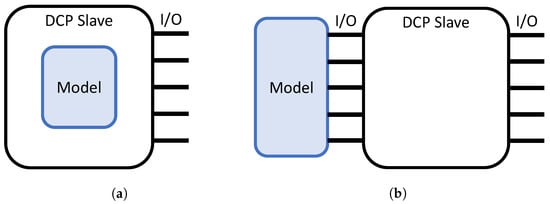
Figure 1.
Comparison between original DCP Secondary design and our interface. (a) Original DCP Secondary design representation: internally linked DCP Secondary and Model, with one specific DCP Secondary for each Model; (b) Proposed interface of new DCP Secondary design: externally linked DCP Secondary and Model, using the same secondary with easily configurable Input/Outputs.
To achieve this independence between the model and the DCP secondary, in addition to implementing a specific DCP secondary, we also developed a series of peripheral modules, which are explained in [7]. Thus, our interface is composed of these modules and a DCP secondary. Our goal in developing this interface as a Simulink library was to take advantage of its tools so that we could generate C/C++ code for our interface and implement it on a variety of hardware platforms without additional modifications.
This modularity, apart from providing flexibility during the design process, allows for the separation of modeling tasks from communication tasks, enabling the user to focus on the system development aspects. Moreover, it extends the applicability of the DCP standard itself, as will be demonstrated later, allowing for the inclusion of technologies such as FPGAs in co-simulations, which is a novel application for the standard. All this contributes to time savings in conducting co-simulations and offers greater adaptability regarding the software and hardware technologies one wishes to employ.
3.1. Configuration of the Interface
We have advanced that the configuration of the interface is based on the DCP standard; therefore, we will use the DCP standard specification document [22] for the explanations of this section. The references to specific clauses of the standard will be in italics to better guide the reader. In this section, we will only focus on the essential parameters (in monospace font) to define our interface; however, there are also other optionally modifiable parameters whose explanation can be found in the standard specification document. Figure 2 will be helpful to understand certain concepts.
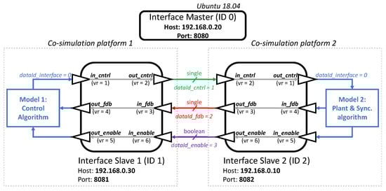
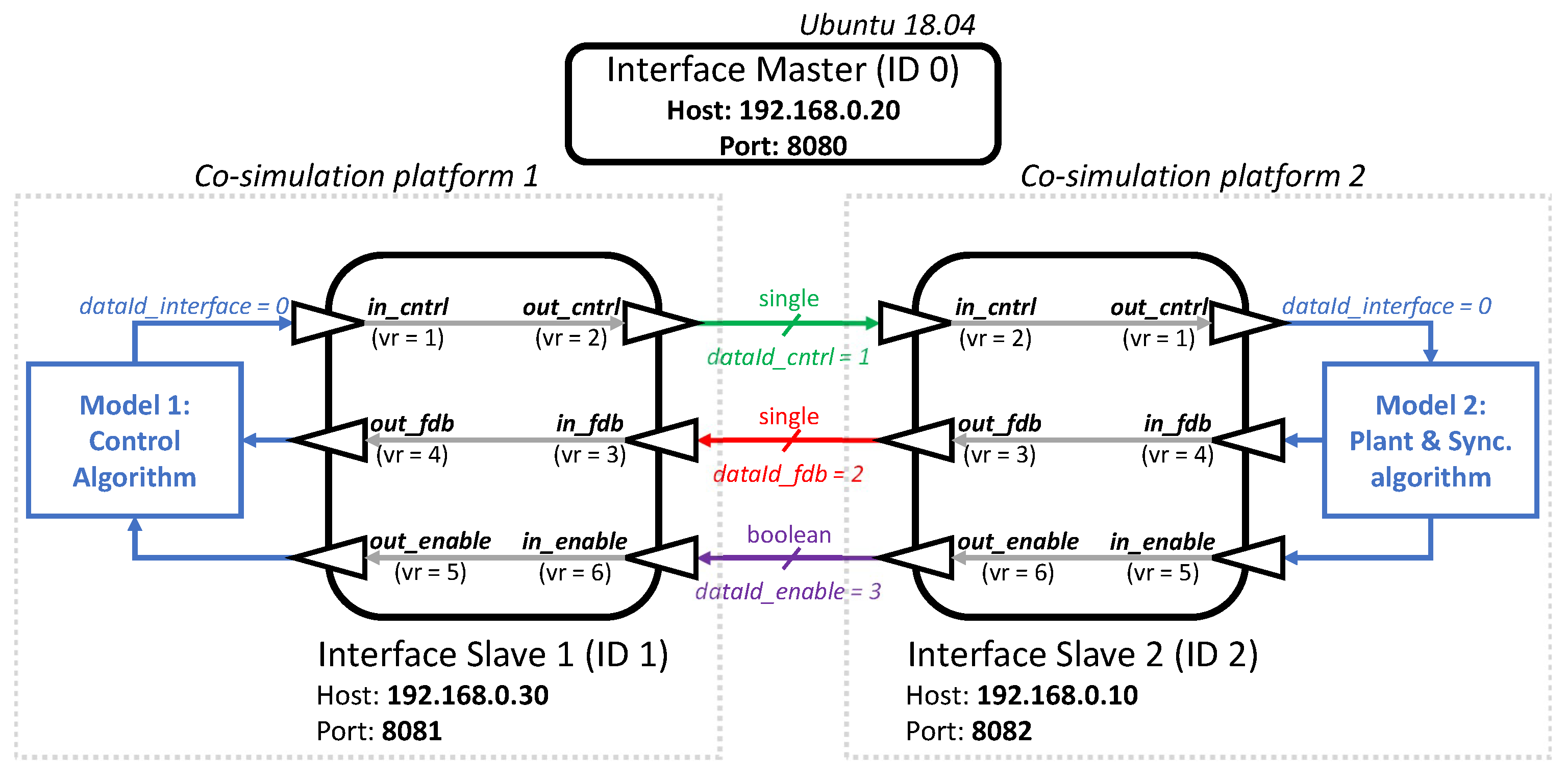
Figure 2.
Interface configuration of the employed use case.
Some parameters are set in each secondary, while others are set in the primary. The secondaries are limited to set their internal parameters (see 5.4 Definition of dcpSlaveDescription Element, pp. 80–82), of which the essential parameters for configuring the interface are defined by the following elements:
- Time resolution (5.9 Definition of TimeRes Element, pp. 87–88). It defines one atomic step of the secondary and is represented by an element that contains a list of permissible single time resolutions or a list of resolution ranges. To set a single resolution, which is what we are going to do next, we have to set two sub-parameters: numerator and denominator, where the numerator divided by the denominator represents the time resolution of the secondary.
- Transport protocol (5.11 Definition of TransportProtocols Element, p. 88). The DCP supports multiple transport protocols and this element is used to store their specific settings. For instance, if the UDP transport protocol is used, this element must indicate it and contain the host and port data of the secondary.
- Variables (5.13 Definition of Variables Element, pp. 92–98). This element contains the information about the variables of the secondary, they can be either an Input, an Output, a Parameter, or a Structural Parameter. Among its sub-parameters, the indispensable ones to configure our interface are valueReference, dataType, and declaredType. valueReference is the identifier of each variable and its value must be unique; in Figure 2, it can be seen how each I/O of each secondary has different valueReference (vr) values. With dataType, we declare the data type of the variable, see Table 174: Data type elements to know the accepted data types by the DCP standard. Finally, with declaredType, we indicate whether the variable is used as an input/output that connects to another secondary, or as an input/output that connects to an external model. For this purpose, we have two predefined options: default, for communication between secondaries, and interface for communication with the models.
As the task of the interface is to communicate between different co-simulation environments, inputs and outputs will always have to be declared in pairs. Each pair will be internally linked in an automatic way as long as their valueReferences are consecutive. In other words, the valueReference parameters of an input–output pair must be consecutive. These values shall consist of the pairs 1–2, 3–4, …, regardless of which of the two is the value of the input and which of the output. Additionally, if an output of one interface communicates with an input of another interface, both must have the same valueReference. This is shown in Figure 2. In this way, we determine the link between interfaces and certify a correct communication.
The primary, on the other hand, configures how the inputs and outputs of the secondaries should communicate with each other. That is to say, it indicates to each secondary where the inputs corresponding to its outputs are and vice versa. In addition, it establishes the sending frequency of each output. To do this, the following parameters must be configured:
- Step Size. The primary defines the step size of each output of all secondaries. The step size is a multiple of the time resolution parameter mentioned in the secondary configuration. That is, the step size of each output is defined by the time resolution of its secondary multiplied by the step parameter.
- Data Identifier (data_id). When exchanging information between secondaries, Outputs are communicated to Inputs via DAT_input_output PDUs. Thanks to the data_id parameter, the values of several outputs of a secondary can be grouped in a single DAT_input_output PDU. Only outputs that have the same configuration, i.e., sender, receiver, and step size, can be grouped together.
4. Methodology
In this section, we explain the experiments that we performed to show how the architecture presented in [6] is applicable on several hardware platforms and how it is applicable on a distributed real-time co-simulation application. To do so, we apply it on four different platforms, which are introduced in Section 4.1. As the proof-of-concept use case, we use a closed-loop control model explained in Section 4.2. In Section 4.3, we present the co-simulation scenarios we use to demonstrate the applicability of the interface. Finally, in Section 4.4, we explain how to configure our generic co-simulation interface for this particular use case.
4.1. Hardware Platforms
In order to test the applicability of our architecture, and thus of our interface, it has been decided to work with hardware platforms designed for different purposes, where concretely we used
- Hardware platforms with integrated FPGA, such as Xilinx Zynq UltraScale+ and Xilinx Zynq-7000 SoC ZC702.
- Hardware platforms with integrated GPU, such as NVIDIA Jetson Nano.
- Generic hardware platforms such as Raspberry Pi 3B, which is very accessible and widely used.
By working with platforms that integrate FPGAs or GPUs, we are able to introduce these technologies into co-simulations, expanding our design to new applications such as simulation accelerators, artificial intelligence, or image processing.
However, for now, our interface has two limitations. Firstly, it is only implemented to run on soft real-time (SRT) and hard real-time (HRT) operation modes, of which the non-real-time (NRT) operation mode has not yet been implemented. Therefore, as both implemented modes require a common clock reference shared by all computing elements, the interface must be implemented in an environment that can provide it. Secondly, for the moment, we have only implemented UDP communication, so the boards must have an Ethernet port.
4.2. Use Case: Control of a Closed-Loop System
As was performed in [7], as a proof of concept, we use a closed-loop control system. This system consists of two parts: a plant, which is modeled as a discrete time first-order system, represented by Equation (1), and a PI control algorithm, represented by Equation (2). The simulation analysis is performed by observing the time evolution of the closed-loop system response to a step input, comparing both the transient and steady-state parts. It is worth pointing out that this work is focused on testing the capability of the interface to communicate distributed systems in real time. Therefore, in order to facilitate the demonstration process, we have chosen this simple use case.
- u is the control signal;
- y is the plant output or feedback signal;
- a is a constant parameter, and it was permanently set to ;
- b is a constant parameter, and it was permanently set to .
- u is the control signal;
- is the proportional gain coefficient;
- is the integral gain coefficient;
- is the sampling period;
- is the error signal;
- is the target reference signal;
- z is the unit delay operator.
4.3. Co-Simulation Scenarios
In [7], we presented different scenarios to explain the development process of the interface. We started with a scenario composed only of Simulink and ended up with a scenario where the control algorithm was running in an UltraScale+ and the plant in Simulink. However, in order to implement the control subsystem on the UltraScale+ board, we manually created a DCP secondary using C++ code that was specifically adapted to work on this board and be compatible with the control algorithm. Now, we want to progress in the development of the interface and test its applicability. To do so, following the MBD methodology, we have automatically generated interface code from the Simulink model, using the Embedded Coder tool. In order to be able to generate code correctly, we adapted the Simulink model by adding blocks and creating functions compatible with this generation. After that, we were able to generate directly implementable code, without the need for any changes, in any of the platforms presented in Section 4.1.
Figure 2 represents the co-simulation scenario. In it, we can see the two models that compose the use case, defined in the Section 4.2, located in different simulation environments and communicated via two entities/secondaries of our interface. On the left, we can see Model 1, where the control algorithm is located. On the right, we can see Model 2, which is composed of the plant and a synchronization mechanism. The latter has the function of ensuring a controlled start of closed-loop control applications. Guaranteeing identical starts in all executions help us analyze the interface behavior. For a detailed description of its operation, refer to [7]. The communication medium used to link both systems is UDP.
To demonstrate the easy implementation capability of the interface on different hardware platforms and, at the same time, to analyze its scope for performing real-time XIL simulations, we have considered the following scenarios:
- Scenario 1.A: Control algorithm and interface in the ARM-based processor of the ZC702 and Plant in Simulink.
- Scenario 1.B: Control algorithm and interface in the ARM-based processor of the UltraScale+ and Plant in Simulink.
- Scenario 2: Control algorithm and interface in the ARM-based processor of the Jetson Nano and Plant in Simulink.
- Scenario 3: Control algorithm and interface in the CPU of the Raspberry-Pi and Plant in Simulink.
- Scenario 4.A: Control algorithm in the FPGA of the ZC702, interface in the ARM-based processor of the ZC702, and Plant in Simulink.
- Scenario 4.B: Control algorithm in the FPGA of the UltraScale+, interface in the ARM-based processor of the UltraScale+, and Plant in Simulink.
Additionally, to demonstrate its applicability in distributed real-time executions, we have proposed the following scenario:
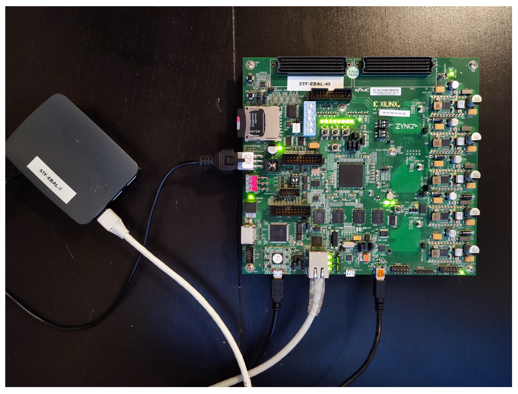
- Scenario 5: Control algorithm in the FPGA of the ZC702, interface in the ARM-based processor of the ZC702, and Plant in the CPU of the Raspberry-Pi, see Figure 3.
 Figure 3. Scenario 5.
It is worth mentioning that in all scenarios, we have kept the same interface configuration (see Section 4.4), thus facilitating the interoperability between simulation tools.
As we mentioned in Section 4.1, our interface is limited to work in real-time operation mode; therefore, all the scenarios have to be executed in real time. The DCP standard defines that in its real-time mode, all components within the simulation must be synchronized with POSIX time. That is to say, they have to synchronize their clock by reference to 1 January 1970, 00:00:00 UTC. Consequently, we have to make all the components run in an environment that supports it and make them synchronized with each other. To make this possible on the platforms, we have installed an Ubuntu operating system on the CPUs of all of them, whose clock will be synchronized with the POSIX time. Therefore, the interface and the system (plant or controller) will run on it. Regarding Simulink, as explained above, by default, it works in non-real-time mode. However, we will use its Simulink Desktop Real-Time tool in I/O mode, which allows us to synchronize the UDP ports with the wall clock. This way, it will be also be synchronized to the POSIX time. It should be noted that we will run Simulink on a conventional PC that contains a 6-core Intel Core i7 CPU processor and uses a Windows 10 operating system.
The use of the interface must not alter the behavior of the closed-loop system in any of the scenarios. Therefore, we need a reference in order to be compared with the scenarios. To this end, using the Embedded Coder and HDL Coder tools provided via Simulink, we conducted Processor-in-the-Loop (PIL) and FPGA-in-the-Loop (FIL) simulations equivalent to the scenarios. In this way, we obtained a reference response for each of the scenarios. In other words, for scenarios 1.A, 1.B, 2, and 3, we performed PIL simulations, one with each hardware platform, while for scenarios 4.A and 4.B, we performed FIL simulations. Each of these simulations are used as a reference for their respective scenario. Regarding scenario 5, we compare its responses to those of the system running entirely in Simulink.
4.4. Interface and Simulations Configuration
Two types of configurations were applied to conduct the experiment: the configuration of the models to be simulated and the configuration of the interface.
Regarding the configuration of the models, in [7], we saw that the behavior of the interface varied depending on the execution time; therefore, we performed the tests using six different configurations. In the current article, instead, we are going to focus on working only with the most limiting configuration that we encountered, which is shown at Table 1.

Table 1.
Configuration for the simulation.
Regarding the configuration of the co-simulation interface. In Section 3.1, we explain the indispensable parameters to be configured. Now, we specify which values we chose for our particular use case:
- Time resolution. With this parameter, we indicate under which step size the state machine of the interface is executed. We set it to the lowest resolution that Simulink Desktop Real-Time allows for when working in I/O mode. Therefore, we set it to 1 ms: and . It is also worth mentioning that the step size of the interface must be lower than that of the model [7].
- Transport protocol. As mentioned, we use UDP. In Figure 2, we can see the chosen host and port values.
- Variables. We declared three inputs and three outputs to each interface. In Figure 2, we can see the data types and the value reference of each one.
- Data identifier. In Figure 2, we can see that each secondary has been assigned four data_id. This means that each variable that is transmitted between secondaries has grouped independently, while the outputs that go from the interfaces to each of the models have been grouped together.
- Step size. We assigned a step value of 3 to the three data_ids that are transmitted between secondaries (i.e., dataId_cntrl, dataId_fdb, and dataId_enable) and a step value of 10 to dataId_interface. With this configuration, we could have assigned the same data_id to the three signals that are transmitted between secondaries, but this makes it easier in case of future modifications.
5. Results
In this section, we present the simulation results of the scenarios explained in Section 4.3. They will be discussed in Section 6. In order to prove that the system behaves identically for every execution, as conducted in [7], we perform 25 executions of each scenario. Between each run, the system is reset in order to ensure identical starting conditions in each of them. Subsequently, we compare the time response of the output of each scenario with the respective reference. From this comparison, we obtain the error, which is calculated by means of Equation (3).
where N represent the steps executed in a simulation, is the response of the closed-loop system at step k under a specific scenario, and is the response of the closed-loop system under the corresponding reference. Table 2 reports the maximum, the minimum, the mean, and the standard deviation of the error over the 25 repetitions.
Table 2.
Comparison between MathWorks PIL/FIL solution and the proposed interface.
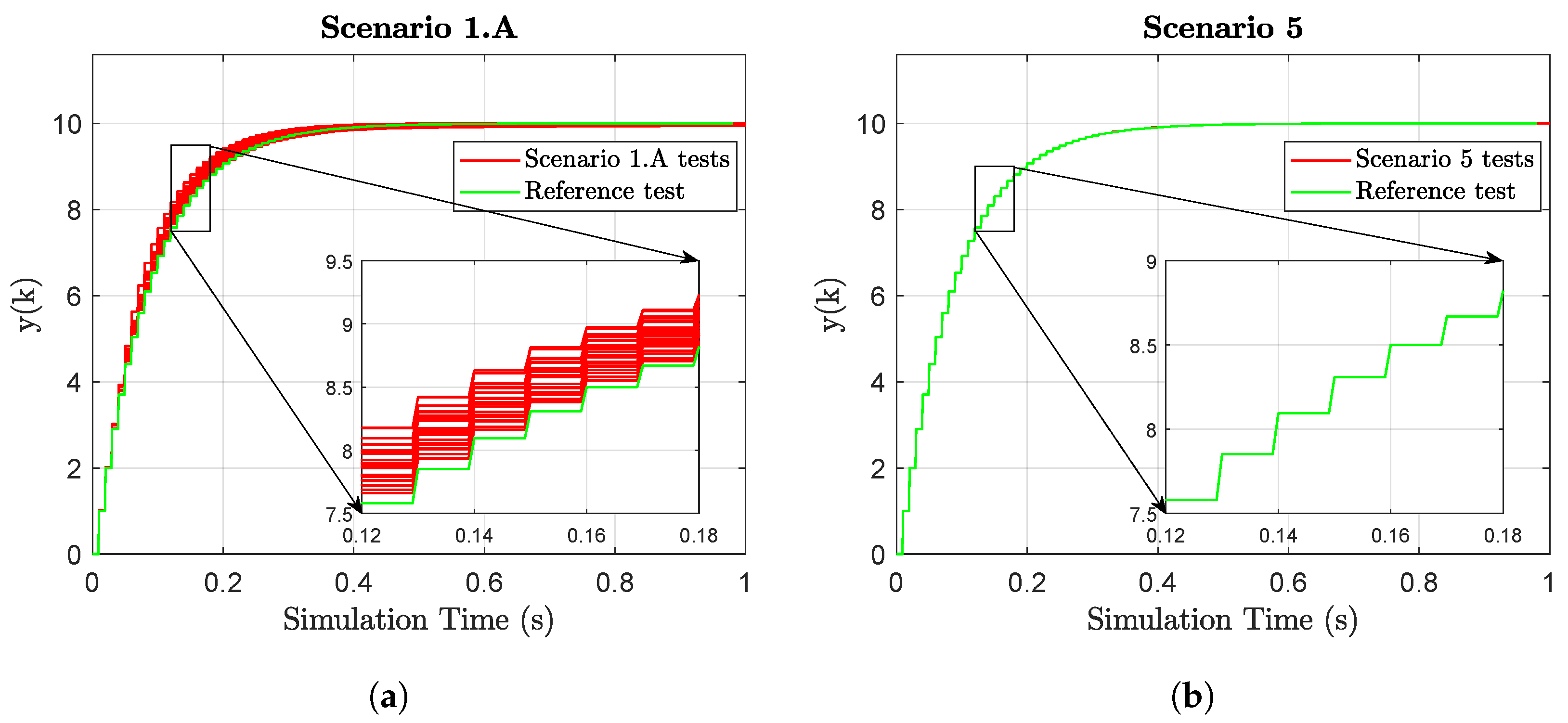
Figure 4 helps us understand the results of the table. It comprises two graphs, each comparing the response of a scenario (red line) with its corresponding reference (green line). There are 25 red lines in each graph, corresponding to the 25 repetitions that were executed for each configuration. We have decided to show only these two scenarios because they are sufficient to explain the behavior of the rest.
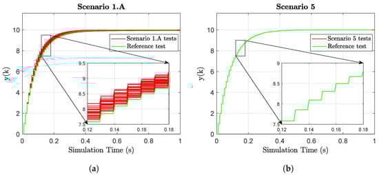
Figure 4.
Comparison of the responses of Scenarios 1A and 5 with their respective References. (a) Scenario 1A. (b) Scenario 5. The responses overlap.
6. Results Analysis
There are three topics we have discussed in this article, so this analysis will also be divided into three parts.
The first point focuses on evaluate the viability and ease of implementation of the interface in a variety of hardware platforms. Since we developed it in Simulink and adapted all its functions to be compatible with the generation of generic C/C++ code, we were able to implement it easily on all the platforms mentioned in Section 4.1. This way we demonstrate that the interface can be migrated between platforms without any extra effort.
As for our second point, we evaluated the viability of the interface to perform real-time executions between Simulink and the platforms described in Section 4.1. In Table 2, from Scenario 1A to Scenario 4.B, we find the results of the tests carried out for this point. Additionally, Figure 4a displays graphically the results obtained in Scenario 1A. As the graphs obtained in Scenarios 1A to 4B are very similar, we decided to omit the rest and display only this one to assist in the interpretation of Table 2. Analyzing this table, we observe that there is an error in every scenario. Simplifying the results, we can say that the mean error of PIL simulations (from Scenarios 1A to 3) is in the order of 0.215 units (), whereas the mean error of FIL simulations (Scenarios 4A and 4B) is about 0.13 units (). This error occurs because the PIL and FIL simulations made with MathWorks tools exhibit identical behavior in each run, while our simulations vary in each of the 25 runs. This can be seen in Figure 4a, where there is single green line (corresponding to the MathWorks response) and multiple red lines (each corresponding to one of the 25 tests). Nevertheless, it can also be seen that this error is focused in the transient state, while in the steady state, it is minimum. In fact, in the steady state, from second 0.4 onwards, the mean error is of the order of 0.019 units (), with a standard deviation of another 0.019 units ().
The appearance of this error means that our solution is not deterministic, which is an indispensable quality in the real-time executions for the verification and validation processes of the CPS. Therefore, we can say that our interface is not suitable for linking Simulink and hardware platforms in real time. However, we did not test how our interface would behave with these scenarios working in non-real-time mode, that is, following the controlled read-compute-write sequence explained previously. In fact, this is the way that MathWorks performs PIL and FIL simulations. Nevertheless, as explained before, this is an operation mode that we have yet to implement.
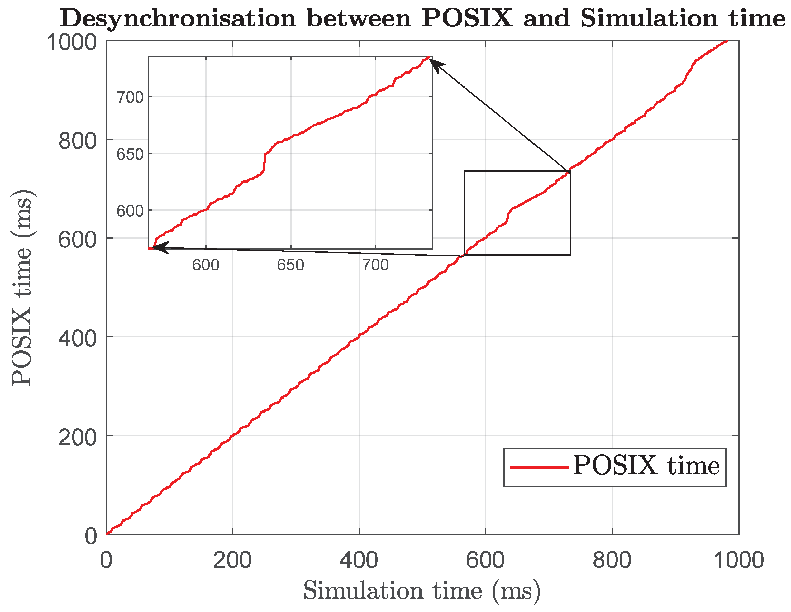
Analyzing the cause of this non-deterministic response, we have not been able to link Simulink simulation time with POSIX time. In other words, POSIX time is constantly moving forward, and in a period of time, the simulation time becomes blocked and it does not advance. Figure 5 demonstrates this behavior, where the graph, instead of showing a perfect diagonal line, shows “jumps”, which are sometimes more pronounced. As we discussed previously, real-time systems must guarantee a response every predefined period and this break does not allow it. This can be caused, for instance, due to an interruption in the computing platform. This is the reason why we have not been able to benefit from all the power that the Simulink Desktop Real-Time tool provides.
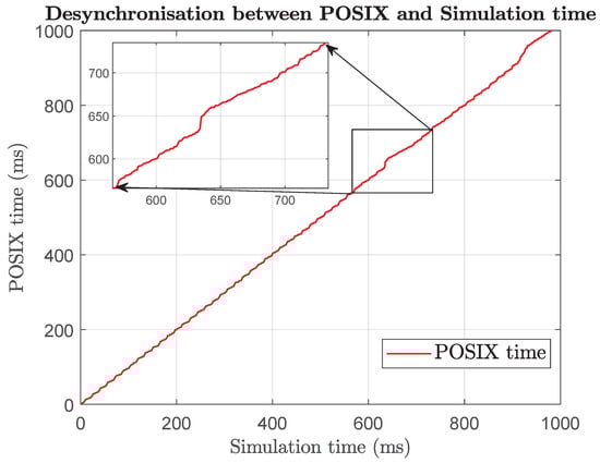
Figure 5.
Desynchronisation between POSIX and Simulation time.
The effect of this desynchronization in our scenarios is that the plant, which is executing in Simulink, stops running for an indefinite period, while the control algorithm on the hardware platform continues to run. During this period, the control will not receive updated input values from the plant; however, they will be processed, provoking incorrect output control signals. When the plant resumes running, it reads the last of this unwanted values, resulting in an incorrect feedback value being sent to the controller. This way, a single desynchronization in the execution can significantly impact the system’s behavior, leading to non-deterministic behavior. It is worth mentioning that the faster the system runs, the smaller its execution steps will be. As a result, a pause in the simulation time will involve more simulation steps, creating a more adverse effect on the system’s response.
Finally, it remains to analyze the response of our implementation in real-time distributed applications, i.e., Figure 4b. Contrary to what happens in the previous tests, we can see how the 25 red lines are overlapped. On top of that, they have the same behavior as the reference (green line). The fact that we obtained identical results in all executions means a deterministic simulation. Therefore, we can be assured that our interface is suitable for real-time distributed simulations. At the same time, these results demonstrate that the problem we had in linking Simulink with hardware platforms lies in the fact we were not able to link Simulink with the wall clock correctly.
7. Conclusions and Future Work
In this paper, we present an empirical demonstration of the applicability of the previously developed generic co-simulation interface. Specifically, we demonstrated (i) its easy implementation on a variety of hardware platforms and (ii) how it can be used in real-time distributed simulations. Both capabilities are very useful in the process of verification and validation of cyber–physical systems, especially in those whose components are developed by different suppliers; in those where the system is split into smaller modules to spread the computational load across different processors; or in those where the integration of different simulators into a single system is required. Therefore, our interface could save time, resources, and money, as it facilitates the coupling of elements, saves displacements for integration testing, and helps to preserve Intellectual Property.
To test the interface, we deployed it in different hardware boards and performed a closed-loop simulation between them, obtaining reliable responses. Consistent with the MBD methodology, as we have developed it in Simulink and take advantage of its code generation capabilities, our interface is easily implementable in a wide variety of simulation environments. Additionally, as our interface is based on the non-proprietary DCP standard, it is fully compatible with any other DCP secondary.
Looking to extend our work to the future, in order to improve the linking capability to Simulink, we want to develop the non-real-time simulation mode. Additionally we have planned to test the applicability of this interface in a more complex use case involving hardware-in-the-loop simulations.
Author Contributions
Conceptualization, M.S., A.J.C., T.P. and R.B.; methodology, M.S. and A.J.C.; software, M.S.; validation, A.J.C., T.P. and R.B.; investigation, M.S.; writing—original draft preparation, M.S.; writing—review and editing, A.J.C., T.P. and R.B.; supervision, T.P. and R.B. All authors have read and agreed to the published version of the manuscript.
Funding
This research was funded by Basque Government through the ELKARTEK programme under the AUTOTRUS project (grant number KK-2023/00019) and the European Commission’s Horizon Europe programme under the METASAT project (grant 101082622).
Data Availability Statement
The data presented in this study are available on request from the corresponding author.
Conflicts of Interest
The authors declare no conflict of interest.
Abbreviations
The following abbreviations are used in this manuscript:
| DCP | Distributed Co-Simulation Protocol |
| MBD | Model-based design |
| CPS | Cyber–physical system |
| M&S | Modeling and simulation |
| XIL | X-in-the-Loop |
| MIL | Model-in-the-Loop |
| SIL | Software-in-the-Loop |
| PIL | Processor-in-the-Loop |
| HIL | Hardware-in-the-Loop |
| HIL | FPGA-in-the-Loop |
| UDP | User Datagram Protocol |
| FMI | Functional Mock-up Interface |
| RT | Real-time |
| NRT | Non-real-time |
| SRT | Soft real-time |
| HRT | Hard real-time |
| FPGA | Field-programmable gate array |
| GPU | Graphics processor unit |
References
- Böhm, W.; Broy, M.; Klein, C.; Pohl, K.; Rumpe, B.; Schröck, S. Model-Based Engineering of Collaborative Embedded Systems, 1st ed.; Springer: Berlin/Heidelberg, Germany, 2021; Chapter 12 and 13. [Google Scholar] [CrossRef]
- Marwedel, P. Embedded System Design—Embedded Systems Foundations of Cyber-Physical Systems, and the Internet of Things, 4th ed.; Springer: Berlin/Heidelberg, Germany, 2021; Chapter 1. [Google Scholar] [CrossRef]
- Falcone, A.; Garro, A. Distributed Co-Simulation of Complex Engineered Systems by Combining the High Level Architecture and Functional Mock-up Interface. Simul. Model. Pract. Theory 2019, 97, 101967. [Google Scholar] [CrossRef]
- Alfalouji, Q.; Schranz, T.; Falay, B.; Wilfling, S.; Exenberger, J.; Mattausch, T.; Cláudio Gomes, G.S. Co-simulation for buildings and smart energy systems—A taxonomic review. Simul. Model. Pract. Theory 2023, 126, 102770. [Google Scholar] [CrossRef]
- Attarzadeh-Niaki, S.H.; Sander, I. Heterogeneous co-simulation for embedded and cyber-physical systems design. Simul. Trans. Soc. Model. Simul. Int. 2020, 96, 753–765. [Google Scholar] [CrossRef]
- Segura, M.; Poggi, T.; Barcena, R. Towards the implementation of a real-time co-simulation architecture based on distributed co-simulation protocol. In Proceedings of the 35th Annual European Simulation and Modelling Conference 2021, ESM 2021, EUROSIS-ETI, Rome, Italy, 27–29 October 2021; pp. 155–162. [Google Scholar]
- Segura, M.; Poggi, T.; Barcena, R. A Generic Interface for x-in-the-Loop Simulations Based on Distributed Co-Simulation Protocol. IEEE Access 2023, 11, 5578–5595. [Google Scholar] [CrossRef]
- Hrvanovic, D.; Haberl, H.; Krammer, M.; Scharrer, M.K. Distributed Co-Simulation for Effective Development of Battery Management Functions. SAE Int. 2023. [Google Scholar] [CrossRef]
- Mihal, P.; Schvarcbacher, M.; Rossi, B.; Pitner, T. Smart grids co-simulations: Survey & research directions. Sustain. Comput. Inform. Syst. 2022, 35, 100726. [Google Scholar] [CrossRef]
- Köhler, C. Enhancing Embedded Systems Simulation, 1st ed.; Vieweg+Teubner: Wiesbaden, Germany, 2011; Book 2. [Google Scholar] [CrossRef]
- Baumann, P.; Krammer, M.; Driussi, M.; Mikelsons, L.; Zehetner, J.; Mair, W.; Schramm, D. Using the Distributed Co-Simulation Protocol for a Mixed Real-Virtual Prototype. In Proceedings of the 2019 IEEE International Conference on Mechatronics, ICM 2019, Ilmenau, Germany, 18–20 March 2019; pp. 440–445. [Google Scholar] [CrossRef]
- Ivanov, V.; Augsburg, K.; Bernad, C.; Dhaens, M.; Dutré, M.; Gramstat, S.; Magnin, P.; Schreiber, V.; Skrt, U.; Kelecom, N.V. Connected and shared x-in-the-loop technologies for electric vehicle design. World Electr. Veh. J. 2019, 10, 83. [Google Scholar] [CrossRef]
- Sagardui, G.; Agirre, J.; Markiegi, U.; Arrieta, A.; Nicolás, C.F.; Martín, J.M. Multiplex: A co-simulation architecture for elevators validation. In Proceedings of the IEEE International Workshop of Electronics, Control, Measurement, Signals and their Application to Mechatronics (ECMSM), Donostia, Spain, 24–26 May 2017; pp. 1–6. [Google Scholar] [CrossRef]
- Çakmak, H.; Erdmann, A.; Kyesswa, M.; Kühnapfel, U.; Hagenmeyer, V. A new distributed co-simulation architecture for multi-physics based energy systems integration. Automatisierungstechnik 2019, 67, 972–983. [Google Scholar] [CrossRef]
- Hatledal, L.I.; Styve, A.; Hovland, G.; Zhang, H. A Language and Platform Independent Co-Simulation Framework Based on the Functional Mock-Up Interface. IEEE Access 2019, 7, 109328–109339. [Google Scholar] [CrossRef]
- Ali, M.; Mohamed, E.; Wu, L.; AbouRizk, S. A generic framework for simulation-based optimization using high-level architecture. In Proceedings of the Proceedings of the 21st International Conference on Modelling and Applied Simulation (MAS 2022), Rome, Italy, 19–21 September 2022. [Google Scholar] [CrossRef]
- Modelica Association. Distributed Co-Simulation Protocol (DCP) Website. 2023. Available online: https://dcp-standard.org/ (accessed on 3 December 2023).
- Modelica Association. DCP Library. 2023. Available online: https://github.com/modelica/DCPLib (accessed on 3 December 2023).
- Kopetz, H. Real-Time Systems, 2nd ed.; Real-Time Systems Series; Springer: New York, NY, USA, 2011; pp. XVIII, 378. [Google Scholar] [CrossRef]
- MathWorks. Simulink Desktop Real-Time. 2023. Available online: https://es.mathworks.com/help/sldrt/low-sample-rate-simulation.html (accessed on 3 December 2023).
- Krammer, M.; Kater, C.; Schiffer, C.; Benedikt, M. A Protocol-Based Verification Approach for Standard-Compliant Distributed A Protocol-Based Verification Approach for Standard-Compliant Distributed Co-Simulation. In Proceedings of the Asian Modelica Conference 2020, Tokyo, Japan, 8–9 October 2020. [Google Scholar] [CrossRef]
- Modelica Association. DCP Standard Specification. 2023. Available online: https://github.com/modelica/dcp-standard (accessed on 3 December 2023).

Disclaimer/Publisher’s Note: The statements, opinions and data contained in all publications are solely those of the individual author(s) and contributor(s) and not of MDPI and/or the editor(s). MDPI and/or the editor(s) disclaim responsibility for any injury to people or property resulting from any ideas, methods, instructions or products referred to in the content. |
© 2023 by the authors. Licensee MDPI, Basel, Switzerland. This article is an open access article distributed under the terms and conditions of the Creative Commons Attribution (CC BY) license (https://creativecommons.org/licenses/by/4.0/).