
Inversion of Target Magnetic Moments Based on Scalar Magnetic Anomaly Signals

1
Aerospace Information Research Institute, Chinese Academy of Sciences, Beijing 100190, China
2
Key Laboratory of Electromagnetic Radiation and Sensing Technology, Chinese Academy of Sciences, Beijing 100190, China
3
School of Electronic, Electrical and Communication Engineering, University of Chinese Academy of Sciences, Beijing 100190, China
*
Author to whom correspondence should be addressed.
Electronics 2023, 12(24), 4900; https://doi.org/10.3390/electronics12244900
Submission received: 12 October 2023
/
Revised: 29 November 2023
/
Accepted: 2 December 2023
/
Published: 5 December 2023
(This article belongs to the Section Circuit and Signal Processing)
Abstract
:As a key physical property of underwater ferromagnetic targets, magnetic moment can reflect important information such as the mass and heading of the target. However, most of the current magnetic moment estimation methods rely on vector magnetic field sensors or sensor arrays to measure the magnetic field, which limits its application in remote target magnetic moment calculation on mobile platforms to some extent. To solve this problem, a real-time magnetic moment inversion method based on the high-precision scalar magnetic measurement data of a high-speed moving platform is proposed in this paper. The method allows the estimation of the magnetic moment of underwater ferromagnetic targets by the scalar magnetic measurement data of an optical pump magnetic field sensor mounted on a high-speed moving platform. The experimental results show that this method has high precision in estimating magnetic moment; the average error of the magnetic moment amplitude was only 5.85%, while the average errors of the magnetic moment inclination and magnetic moment deflection were 1.58° and 2.79°, respectively. These results provide a new and effective way to estimate the magnetic moment of underwater ferromagnetic targets and are expected to have important practical applications.
1. Introduction
Ferromagnetic targets are important monitored objects in the marine field, and the detection and recognition [1] of underwater ferromagnetic targets are of great significance in military defense. Magnetic anomaly detection (MAD) [2] is the process of detecting underwater and underground targets using magnetometers to obtain magnetic anomaly information. As the main method of magnetic anomaly detection, aeromagnetic surveys are widely used in mineral exploration [3], submarine detection [4], and unexploded object detection [5,6] due to their advantages [7,8] of high accuracy, high efficiency, all-weather operation, and large operation range.
Over the years, many researchers have studied ferromagnetic target localization. Wynn [9] proposed an eigenvector-based method for magnetic dipole localization. Nara [10] proposed a method for localizing magnetic dipoles by measuring magnetic field vectors and spatial gradients. Wiegert [11] proposed the Scalar Triangulation and Ranging (STAR) method based on the contraction properties of the magnetic gradient tensor for high real-time ferromagnetic target localization. Yang [12] and Yin [13,14] localized the magnetic dipoles using the Normalized Source Strength (NSS). Xu [15] proposed a linear method for magnetic dipole localization based on the full tensor of two-point magnetic gradients.
However, due to the high-speed flight characteristics of aircraft, it is often impossible to track the target as soon as it is detected. Therefore, in addition to localizing the target, it is particularly important to estimate information such as the direction and speed of its motion. The magnetic anomaly signal generated by a remote magnetic target depends only on the position and magnetic moment of the target. The magnetic moment is an important physical parameter of ferromagnetic targets, and its amplitude reflects the volume of the target, while the direction is closely related to the heading of the target. Therefore, the estimation of the direction of the magnetic moment has been the focus of scholars’ attention.
In 2006, Wiegert and Oeschger [16] calculated the magnetic moments with an array of seven low-noise fluxgate magnetometers, and the average estimation error of the magnetic moment direction was less than 13°. In 2008, Sheinker [17] proposed a group method based on incremental learning to estimate the target magnetic moment, and the magnetic moment estimation error was less than 20%. In 2019, Shao and Tang [18] estimated the magnetic moment direction using an array of 16 magnetometers distributed in a volume of 380 mm × 270 mm × 240 mm with an average error of 12°; this method requires the sensors to be close to the target, which is suitable for the medical field. In 2020, Wang and Shen [19] proposed a method to achieve magnetic moment estimation by a single vector magnetometer with a magnetic moment direction estimation error of about 3.5°, but the method needs to keep the vector magnetic field sensor fixed, which is not suitable for use on a motion platform. In 2022, Qin [20] proposed a magnetic moment direction estimation method based on signal energy distribution, the main advantage of which is improving the signal-to-noise ratio of target magnetic anomalies, but the accuracy of the estimated magnetic moment direction is not high.
Most of the above magnetic moment estimation methods utilize vector magnetometers or their arrays for magnetic field measurements, but vector magnetometers suffer from the problem of large steering differences, which restricts their application on motion platforms. Therefore, this paper proposes a method to estimate the magnetic moment of an underwater ferromagnetic target based on a scalar magnetometer mounted on a high-speed motion platform. The experimental results show that the method has a high accuracy of magnetic moment estimation, with an average error of 5.85% for magnetic moment amplitude and average errors of 1.58° and 2.79° for magnetic moment tilt and magnetic moment deflection, respectively. The results provide a new method for the magnetic moment estimation of underwater ferromagnetic targets, which is expected to have important practical applications.
2. Principles and Methods
An aeromagnetic survey is a method of detecting magnetic anomalies using magnetic field sensors on aircraft platforms. Because of the advantages of this method, such as high efficiency and wide operating range, it is widely used in such fields as aeromagnetic surveys [21], mineral resource exploration [22], and unexploded ordnance detection [23,24].
Aeromagnetic surveys are a means of long-range detection; the distance between an aircraft and the target is generally far. To simplify the calculation, the target can usually be equivalent to a magnetic dipole with a specific magnetic moment. Previous results showed that the magnetic dipole model can effectively approximate the far-field distribution of ferromagnetic targets when the detection distance is 2~3 times larger than the target size [25]. Therefore, studying the magnetic field distribution of the magnetic dipole is helpful to analyze the solution of the magnetic moment.
2.1. Magnetic Field Distribution of Magnetic Dipoles
The magnetic field generated by a magnetic dipole at the origin at any point-of-space coordinate r can be expressed as [26]:
where is the vector magnetic moment of the magnetic dipole, represents the permeability in a vacuum, and r = |r|.
As shown in Figure 1, the magnetic field generated by the magnetic dipole is superimposed with the local geomagnetic field , and the real magnetic field B in space r is the result of the superposition of the two, that is:
The magnetometer carried on the aircraft is generally a high-sensitivity scalar magnetic field sensor, and its magnetic field measurement value is the amplitude of B, which can be expressed as:
where is the angle between the magnetic field vector and the magnetic anomaly vector . The geomagnetic field amplitude is much greater than the target signal amplitude of the magnetic anomaly, so:
Then, Equation (3) can be simplified as follows:
According to Equation (5), the influence of the amplitude and direction of the magnetic moment on the magnetic field distribution of the magnetic dipole is analyzed.
To facilitate the subsequent description, it is necessary to know the following definitions of inclination and declination. Taking the magnetic field vector B as an example, as shown in Figure 2a, the angle I between the magnetic field and the horizontal plane is known as the magnetic field inclination, and the angle D between the horizontal component of the magnetic field and the due north direction is known as the magnetic field declination. Similarly, in this paper, the inclination and declination of the magnetic moment are denoted by and , respectively, as shown in Figure 2b.
Assuming that the magnetic dipole is located at the origin, the simulation results of the magnetic field distribution in the horizontal plane 300 m above it are shown in Figure 3 and Figure 4. In the figures, represents the amplitude of the magnetic moment, represents the inclination of the magnetic moment, and represents the declination of the magnetic moment.
According to the two figures, the distribution of the position of the extreme point of the magnetic field is related to the direction of the magnetic moment, while the size of the extreme value of the magnetic field is closely related to the amplitude of the magnetic moment. Theoretically, the magnetic field distribution corresponding to each group of magnetic moment parameters is unique, which is the premise of calculating the magnetic moment according to the magnetic measurement data.
2.2. Principle of Aeromagnetic Anomaly Detection
As shown in Figure 5, it is assumed that a ferromagnetic target body is located at the origin O of the coordinate system. During magnetic anomaly detection, the aircraft carrying the magnetic sensor flies along line L above the target to obtain a set of real-time magnetic measurement data containing the target magnetic anomaly field. The change in the geomagnetic field is generally gentle. If there is a ferromagnetic target below the detection position, the magnetic anomaly field it generates at the detection position is superimposed with the geomagnetic field, so that the magnetic anomaly appears in the magnetic measurement data. According to this feature, it can be determined whether there is a ferromagnetic target nearby. (In Figure 5, h is the vertical height of trajectory L relative to the target, and R is the shortest distance between the target and line L).
Assuming that the equivalent magnetic moment of the ferromagnetic target at O is m = (mx, my, mz)T, the magnetic field sensor position is r = (x, y, z)T, and the target magnetic anomaly = (Bx, By, Bz)T. According to Equation (1), the magnetic anomaly field generated by the target in space can be expressed as:
The vector magnetic field sensor has a low sensitivity and a large steering difference, so the magnetic field measurement is noisy when installed on a moving platform, and it is not suitable for the detection of remote targets. At present, the magnetic field sensors used for target detection on aircraft are mostly scalar magnetic field sensors.
The value of the magnetic anomaly detected by the scalar magnetic field sensor is approximately the projection of the magnetic anomaly vector in the direction of the geomagnetic field. Assuming that the geomagnetic field vector is T = (Tx, Ty, Tz)T, according to Equation (5), the magnetic anomaly signal measured by the scalar magnetic field sensor can be expressed as:
In Equation (7), s is the scalar magnetic anomaly signal. In the actual measurement, the magnetic anomaly signal is superimposed with the geomagnetic field. Therefore, before magnetic anomaly detection, it is necessary to filter out the geomagnetic field. Then, the correlation detection algorithm based on the orthogonal basis function is used to determine whether there is a target.
2.3. Proposed Method
According to the above analysis, the scalar magnetic anomaly signal is only related to the magnetic moment of the target, the location of the target, and the geomagnetic field at the location of the magnetic sensor. Substituting Equation (6) into Equation (7):
Assuming that:
Then, Equation (8) can be written as:
According to Equation (10), if kx, ky, and kz are known, the scalar magnetic anomaly signal is approximately linear with the three components of the magnetic moment. Therefore, the solution of the magnetic moments can be achieved by solving an overdetermined system of equations. Assuming that there are a total of N data points in the obtained measurement data, the magnetic anomaly signal sequence can be expressed as:
Assuming that:
where , .
The magnetic moment is solved by the least squares method, as follows:
However, the x, y, and z in Equation (9) are unknown, so Equation (11) cannot be directly applied to solve for the magnetic moment. When conducting aeromagnetic surveys, the target recognition algorithm can provide an approximate location of the target, which can be used to search the nearby space to determine the location of the target and solve the magnetic moment.
A search space is defined, as shown in Figure 6, and the target position given by the recognition algorithm is taken as the origin of the coordinate system. The position of the magnetic sensor is assumed to be ,, and the real position of the target is . Any point within the search space is selected, and it is assumed to be the target position. The magnetic moment is calculated according to Equation (11).
To determine which point in the search space is closest to the target location, a cost function needs to be defined. The magnetic anomaly signal sequence is calculated by the solved m’ as follows:
If the selected point is just the real position of the target, the deviation between and is almost zero in the case of no noise. On the contrary, the larger the position deviation between the point and the target, the larger the error between and . Therefore, the cost function can be defined as:
The inversion error is minimized when the value of the cost function converges to the minimum value, and the error between point and point is minimized.
A magnetic moment with an amplitude of A·m2, an inclination angle of 10°, and a deflection angle of 30° is taken as an example to simulate the north–south magnetic anomaly signal in a plane with a height of 300 m. The target is located at (0 m, 0 m, 0 m), and the distribution of the cost function with the preset target location is shown in Figure 7, where x represents the north distance difference between the preset target and the real target, y represents the east distance difference between the preset target and the real target, z represents the vertical distance difference between the preset target and the real target, and J represents the value of the cost function. Figure 7 shows that the cost function is convex and converges to a minimum at the target location.
3. Results
3.1. Analysis of Magnetic Moment Inversion Error
According to the theory of magnetic moment inversion above, the scalar magnetic field measurements are numerically approximated in this paper, which introduces errors to the magnetic moment inversion. To verify the effectiveness of the magnetic moment inversion, the proposed method was used to invert the magnetic moments of typical targets in different heading directions.
According to the magnetic moment estimation method in [27], a target with a length of 100 m and a width of 15 m is equivalent to the ellipsoidal shell model with a wall thickness of 0.08 m in the short axis direction and a relative magnetic permeability of 200; thus, one can calculate the magnetic moment vector of the target in the background magnetic field with a magnetic induction amplitude of 46,000 nT, a magnetic inclination of 25°, and a magnetic declension of −2°. The calculated result of the target magnetic moment is shown as the red line in Figure 8, and the magnetic moment inversion error results are presented in Figure 9, where mamp, Im, and Dm denote the magnetic moment amplitude, inclination, and declivity, while Δmamp, ΔIm, and ΔDm denote the inversion errors of magnetic moment amplitude, inclination, and declivity, respectively. The average inversion errors for the magnitude, inclination, and declination of magnetic moment are recorded in Table 1.
Taking the target position as the origin of the coordinate system, we assume that the geomagnetic field vector in the target area remains constant. The aircraft passes directly above the target, traveling from south to north at a speed of 100 m/s, with the closest distance between the aircraft and the target being 300 m. Additionally, the magnetic field sampling rate is 10 Hz.
On the basis of the aircraft position and the scalar magnetic anomaly signal with the background magnetic field removed, the magnetic moments of each heading of a typical target are retrieved, and the result is shown in Figure 8 as the green dashed line. The inversion error plot is shown in Figure 9. The magnetic moment amplitude inversion error was about 0.025% of the true amplitude, the inclination error was about 0.0012°, and the deflection error was about 0.0284°. These errors were caused by the projection of the vector magnetic anomaly signal into the direction of the geomagnetic field, a desirable result in the absence of noise.
3.2. Magnetic Moment Inversion Experiment
In the simulation verification of the magnetic moment inversion algorithm proposed in this paper, we put forward three assumptions:
- 1.
- The geomagnetic field is constant;
- 2.
- The airplane flies strictly on a straight course;
- 3.
- The magnetic anomaly signal is not affected by noise.
Therefore, the inversion error of magnetic moment in this case was only caused by the error introduced when the magnetic anomaly signal is projected to the direction of the geomagnetic field. However, these three assumptions are not valid in the actual aeromagnetic survey: (1) the geomagnetic field changes slowly with the change of time and space, and there is geomagnetic noise covering the target detection band, which pollutes the magnetic anomaly signals; (2) the flight trajectory of the aircraft is not strictly a straight line in the actual flight, which does not introduce noise for the inversion of the magnetic moment. However, the positioning accuracy of the aircraft’s positioning system will introduce a certain error into the magnetic moment inversion; (3) when the aircraft is in flight, the magnetic interference of the on-board electronic equipment and the maneuvering magnetic interference caused by the small changes in the aircraft’s attitude pollute the magnetic anomaly signals, which introduces error into the magnetic moment inversion. Therefore, before the magnetic moment inversion through the magnetic anomaly signal, it is necessary to reduce the noise of the magnetic anomaly signal. First, the energy of the magnetic anomaly signals we are concerned with is mainly distributed in the bandwidth range of 0.04~0.3 Hz, so most of the noise can be removed by band-pass filtering of the aeromagnetic data; in addition, the maneuvering magnetic interference caused by changes in aircraft attitude can be eliminated by the Towlles–Lawson model [28]. The noise reduction processing flow for the aeromagnetic data is shown in Figure 10. In the figure, LPF, HPF, and BPF denote low-pass filtering, high-pass filtering, and band-pass filtering, respectively, and the compensation coefficients are derived from the calibrated flight data. The output data are the magnetic field data after removing the noise outside the target magnetic anomaly band and the maneuvering magnetic interference, which is used for magnetic moment inversion.
To test the performance of the inversion algorithm in magnetic field measurement data containing noise, an aeromagnetic survey was conducted in Hainan, China, with a certain type of aircraft. The scalar magnetometer carried on the aircraft was an optical pump magnetometer with the parameters shown in Table 2. The fluxgate magnetometer in Table 2 was used to record the flight attitude of the aircraft.
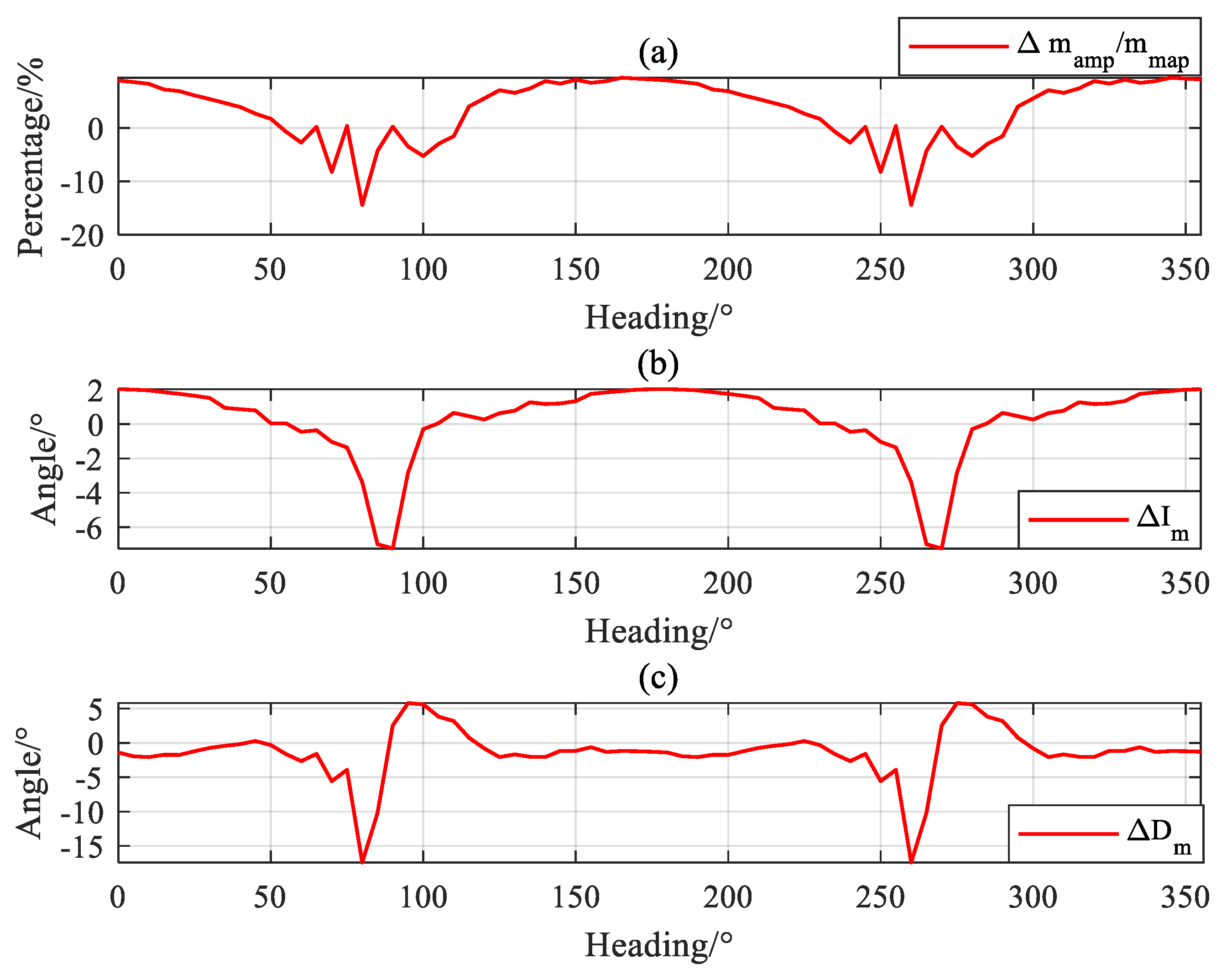
The aircraft flew in a north–south direction at an altitude of approximately 300 m. The target magnetic anomaly signal was added to the magnetic measurement data, and the inversion of the magnetic moments was performed by the method proposed in this paper. The inversion results are shown in Figure 11, and the inversion errors are shown in Figure 12. The average inversion errors for the magnitude, inclination, and declination of the magnetic moment are recorded in Table 3.
According to Figure 12, the magnetic moment amplitude inversion error was about 5.85% of the true amplitude, the inclination error was about 1.58°, and the inclination error was about 2.79°. The error of the inverted magnetic moment was larger when the target heading was near the east–west direction. The east-west component of the geomagnetic field in Hainan, China, is very small. Therefore, when the target sailed along the east–west direction, the magnetization of the geomagnetic field on the target was weak, resulting in a smaller equivalent magnetic moment of the target. Thus, the signal-to-noise ratio of the magnetic anomaly signal was lower, which led to an increase in the inversion error.
4. Discussion
According to the experimental results, the magnetic moment estimation error is related to the signal-to-noise ratio of the magnetic anomaly signal. To allow the proposed method to have better practical applications, it is necessary to reduce the aeromagnetic noise as much as possible. However, in addition to aeromagnetic detection equipment, many aircraft also carry various types of detection equipment, such as radar detection systems, sonar detection systems, and photoelectric detection systems. This inevitably causes severe interference with the aeromagnetic detection data, which makes it difficult for the aeromagnetic compensation program to have a good effect and reduces the magnetic anomaly detection performance. Therefore, to optimize the performance of the aeromagnetic detection equipment, it is necessary to provide a special low-noise flight platform for magnetic exploration equipment.
In addition, the magnetic moment orientation of the underwater target is closely related to its heading, so it is expected to roughly determine the direction of target movement through the magnetic moment orientation in the future.
5. Conclusions
The detection and identification of underwater ferromagnetic targets is an important research direction in the field of national defense, which is of great significance for improving the country’s military defense capability and maintaining national security. Since underwater targets are more hidden, and general detection methods are difficult to perform, these targets are usually detected by aeromagnetic surveys. However, due to the high speeds of vehicles during aeromagnetic surveys, the target cannot be tracked immediately after detection, so it is particularly important to determine the direction of target movement through a magnetic anomaly signal. Magnetic moment, the physical source of the magnetic anomaly signal, is closely related to the target’s heading, so the estimation of the target’s magnetic moment is of great significance for the determination of the target’s heading. In this paper, the magnetic field data obtained by the scalar magnetometer mounted on the flight platform was used to invert the magnetic moment of the ferromagnetic target, which effectively avoided the problem that the vector magnetometer could not be used for the motion platform due to the large steering difference of the vector magnetometer. The experimental results showed that the accuracy of the magnetic moment estimation of the method proposed in this paper is better than that of previous methods, which is of reference significance to promote improvement in the performance of the ferromagnetic target heading recognition algorithm.
Author Contributions
Conceptualization, K.Z.; methodology, K.Z. and X.Y.; software, K.Z.; validation, X.Y., J.L. and X.L.; formal analysis, K.Z. and X.L.; investigation, J.L. and X.L.; resources, W.Z.; data curation, X.Y. and X.L.; writing—original draft preparation, K.Z.; writing—review and editing, X.Y., X.L. and J.L.; visualization, X.Y. and X.L.; supervision, W.Z.; project administration, W.Z.; funding acquisition, W.Z. All authors have read and agreed to the published version of the manuscript.
Funding
This research was funded by the National Key Research and Development Program of China, grant number 2021YFB3900202.
Data Availability Statement
Data are contained within the article.
Acknowledgments
The authors would like to thank the editors and reviewers for their efforts in helping with the publication of this work.
Conflicts of Interest
The authors declare no conflict of interest.
References
- Zhang, C. Some problems concerning the magnetic anomaly detection (MAD). Chin. J. Eng. Geophys. 2007, 4, 549–553. [Google Scholar]
- Sheinker, A.; Ginzburg, B.; Salomonski, N.; Dickstein, P.A.; Frumkis, L.; Kaplan, B.-Z. Magnetic anomaly detection using high-order crossing method. IEEE Trans. Geosci. Remote Sens. 2011, 50, 1095–1103. [Google Scholar] [CrossRef]
- Gunn, P.; Dentith, M. Magnetic responses associated with mineral deposits. AGSO J. Aust. Geol. Geophys. 1997, 17, 145–158. [Google Scholar]
- Hirota, M.; Furuse, T.; Ebana, K.; Kubo, H.; Tsushima, K.; Inaba, T.; Shima, A.; Fujinuma, M.; Tojyo, N. Magnetic detection of a surface ship by an airborne LTS SQUID MAD. IEEE Trans. Appl. Supercond. 2001, 11, 884–887. [Google Scholar] [CrossRef]
- Paoletti, V.; Buggi, A.; Pašteka, R. UXO detection by multiscale potential field methods. Pure Appl. Geophys. 2019, 176, 4363–4381. [Google Scholar] [CrossRef]
- Wigh, M.D.; Hansen, T.M.; Døssing, A. Inference of unexploded ordnance (UXO) by probabilistic inversion of magnetic data. Geophys. J. Int. 2020, 220, 37–58. [Google Scholar] [CrossRef]
- Hood, P. History of aeromagnetic surveying in Canada. Lead. Edge 2007, 26, 1384–1392. [Google Scholar] [CrossRef]
- Reford, M.; Sumner, J. Aeromagnetics. Geophysics 1964, 29, 482–516. [Google Scholar] [CrossRef]
- Wynn, W.; Frahm, C.; Carroll, P.; Clark, R.; Wellhoner, J.; Wynn, M. Advanced superconducting gradiometer/magnetometer arrays and a novel signal processing technique. IEEE Trans. Magn. 1975, 11, 701–707. [Google Scholar] [CrossRef]
- Nara, T.; Suzuki, S.; Ando, S. A closed-form formula for magnetic dipole localization by measurement of its magnetic field and spatial gradients. IEEE Trans. Magn. 2006, 42, 3291–3293. [Google Scholar] [CrossRef]
- Wiegert, R.; Oeschger, J.; Tuovila, E. Demonstration of a novel man-portable magnetic STAR technology for real time localization of unexploded ordnance. In Proceedings of the OCEANS 2007, Vancouver, BC, Canada, 29 September–4 October 2007; pp. 1–7. [Google Scholar]
- Yang, Z.; Yan, S.; Chen, L.; Li, B. Ferromagnetic Object Localization Based on Improved Triangulating and Ranging. IEEE Magn. Lett. 2019, 10, 1–5. [Google Scholar] [CrossRef]
- Yin, G.; Li, P.; Wei, Z.; Liu, G.; Yang, Z.; Zhao, L. Magnetic dipole localization and magnetic moment estimation method based on normalized source strength. J. Magn. Magn. Mater. 2020, 502, 166450. [Google Scholar] [CrossRef]
- Yin, G.; Zhang, L.; Jiang, H.; Wei, Z.; Xie, Y. A closed-form formula for magnetic dipole localization by measurement of its magnetic field vector and magnetic gradient tensor. J. Magn. Magn. Mater. 2020, 499, 166274. [Google Scholar] [CrossRef]
- Xu, L.; Gu, H.; Chang, M.; Fang, L.; Lin, P.; Lin, C. Magnetic target linear location method using two-point gradient full tensor. IEEE Trans. Instrum. Meas. 2021, 70, 1–8. [Google Scholar] [CrossRef]
- Wiegert, R.; Oeschger, J. Generalized magnetic gradient contraction based method for detection, localization and discrimination of underwater mines and unexploded ordnance. In Proceedings of the OCEANS 2005 MTS/IEEE, Washington, DC, USA, 17–23 September 2005; pp. 1325–1332. [Google Scholar]
- Sheinker, A.; Salomonski, N.; Ginzburg, B.; Frumkis, L.; Kaplan, B.-Z. Remote sensing of a magnetic target utilizing population based incremental learning. Sens. Actuators A Phys. 2008, 143, 215–223. [Google Scholar] [CrossRef]
- Shao, G.; Tang, Y.; Tang, L.; Dai, Q.; Guo, Y.-X. A Novel Passive Magnetic Localization Wearable System for Wireless Capsule Endoscopy. IEEE Sens. J. 2019, 19, 3462–3472. [Google Scholar] [CrossRef]
- Wang, J.; Shen, Y.; Zhao, R.; Zhou, C.; Gao, J. Estimation of dipole magnetic moment orientation based on magnetic signature waveform analysis by a magnetic sensor. J. Magn. Magn. Mater. 2020, 505, 166761. [Google Scholar] [CrossRef]
- Qin, Y.; Li, M.; Li, K.; Pan, Y.; Yang, X.; Ouyang, J. Target magnetic moment orientation estimation method based on full magnetic gradient orthonormal basis function. AIP Advances. 2022, 12. [Google Scholar] [CrossRef]
- Lemercier, D.; Salvi, A. Method and Device for Determining the Depth of a Magnetic Anomaly. U.S. Patent 3,808,519, 30 April 1974. [Google Scholar]
- Mooney, H.M. Interpretation Theory in Applied Geophysics. Science 1966, 152, 339–340. [Google Scholar] [CrossRef]
- Munschy, M.; Boulanger, D.; Ulrich, P.; Bouiflane, M. Magnetic mapping for the detection and characterization of UXO: Use of multi-sensor fluxgate 3-axis magnetometers and methods of interpretation. J. Appl. Geophys. 2007, 61, 168–183. [Google Scholar] [CrossRef]
- Tantum, S.L.; Yu, Y.; Collins, L.M. Bayesian Mitigation of Sensor Position Errors to Improve Unexploded Ordnance Detection. IEEE Geosci. Remote Sens. Lett. 2008, 5, 103–107. [Google Scholar] [CrossRef]
- Liu, Z.Y.; Pang, H.F.; Pan, M.C.; Wan, C.B. Calibration and Compensation of Geomagnetic Vector Measurement System and Improvement of Magnetic Anomaly Detection. IEEE Geosci. Remote Sens. Lett. 2016, 13, 447–451. [Google Scholar] [CrossRef]
- Jackson, J.D. Classical Electrodynamics, 2nd ed.; Wiley: Hoboken, NJ, USA, 1975. [Google Scholar]
- Wan, C. Investigations on the Theory and Method of Magnetic Anomaly Detection. Ph.D. Thesis, National University of Defense Technology, Changsha, China, 2018. [Google Scholar]
- Tolles, W.E.; Lawson, J. Magnetic Compensation of MAD Equipped Aircraft; Airborne Instrum. Lab. Inc., Mineola NY Rept: Georgetown, TX, USA, 1950; p. 201. [Google Scholar]
Figure 1.
Schematic diagram of superposition of geomagnetic field and interference magnetic field.
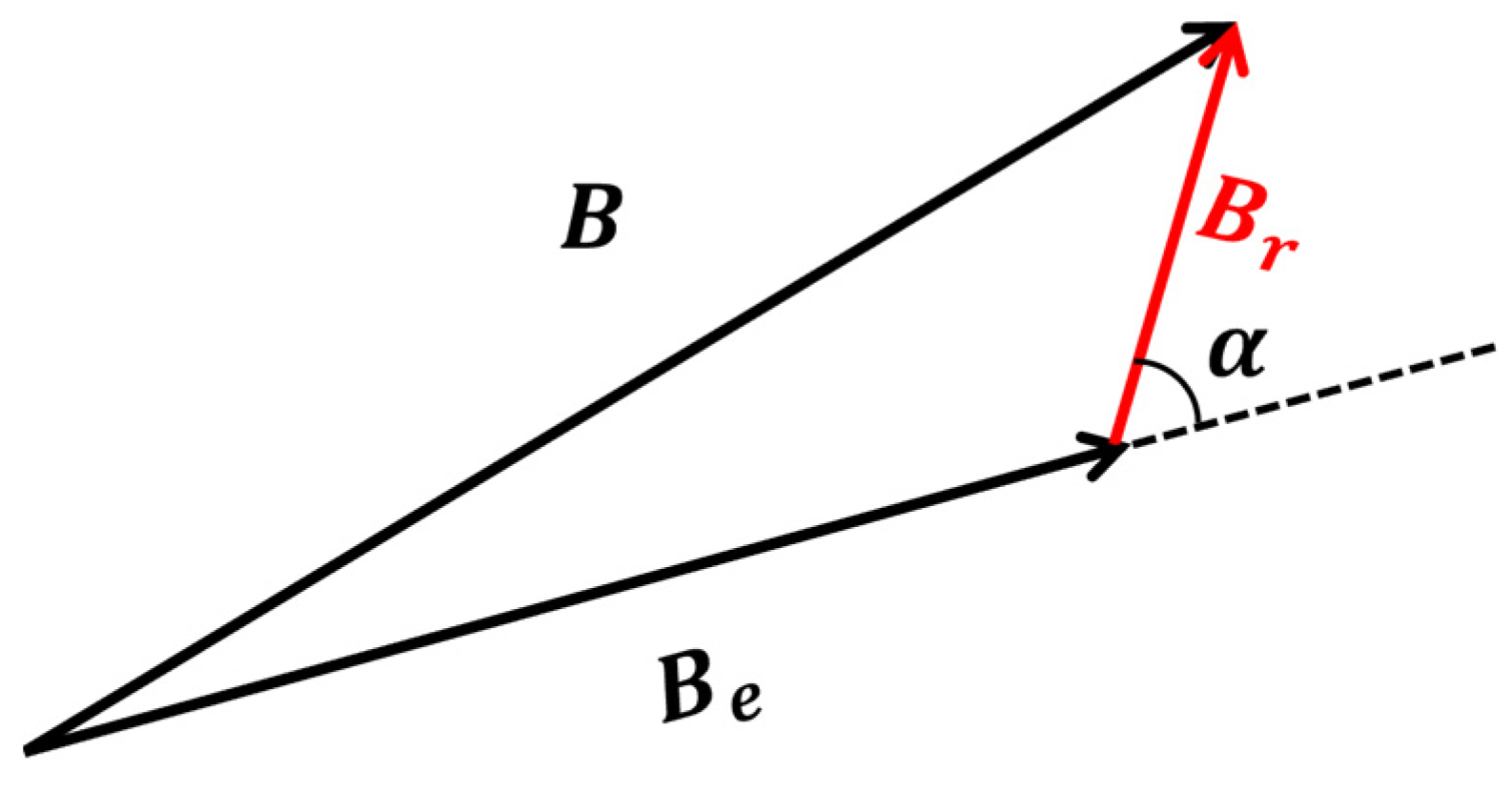
Figure 2.
Schematic diagram of inclination and declination: (a) Schematic diagram of the inclination and declination angles of the magnetic field; (b) Schematic diagram of the inclination and declination angles of the magnetic moment.
Figure 2.
Schematic diagram of inclination and declination: (a) Schematic diagram of the inclination and declination angles of the magnetic field; (b) Schematic diagram of the inclination and declination angles of the magnetic moment.
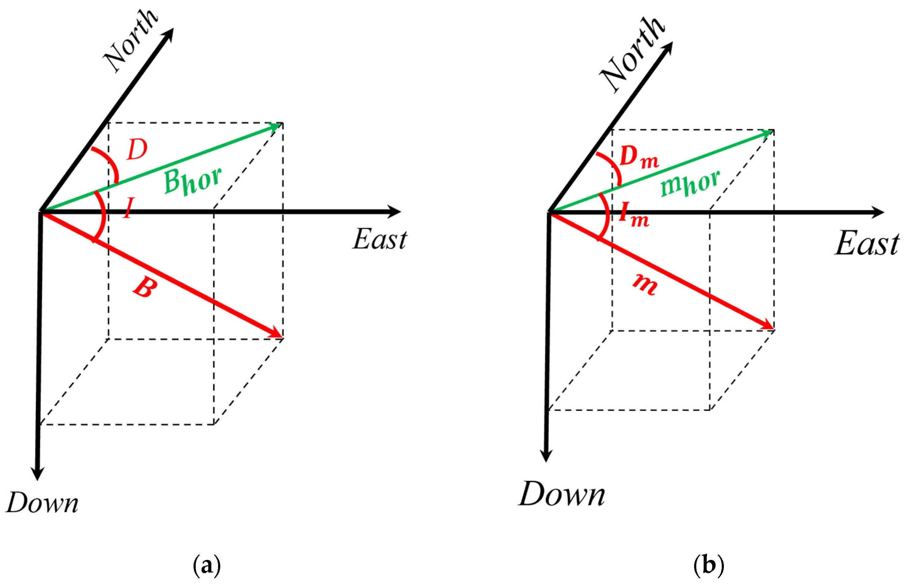
Figure 3.
Effect of magnetic moment direction on magnetic field distribution of magnetic dipole.

Figure 4.
Effect of magnetic moment amplitude on magnetic field distribution of magnetic dipole.
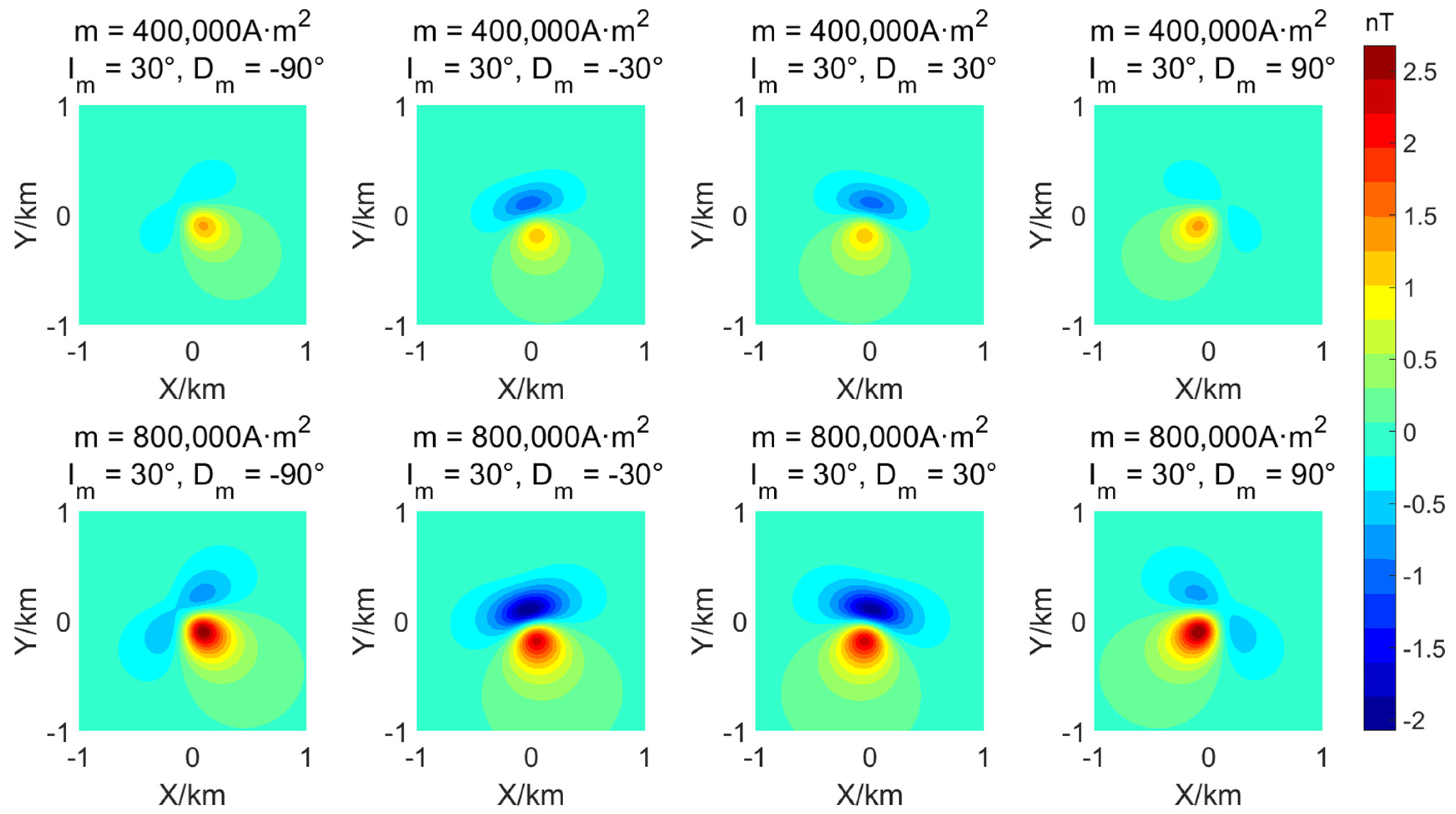
Figure 5.
Schematic diagram of the principle of aeromagnetic measurement.
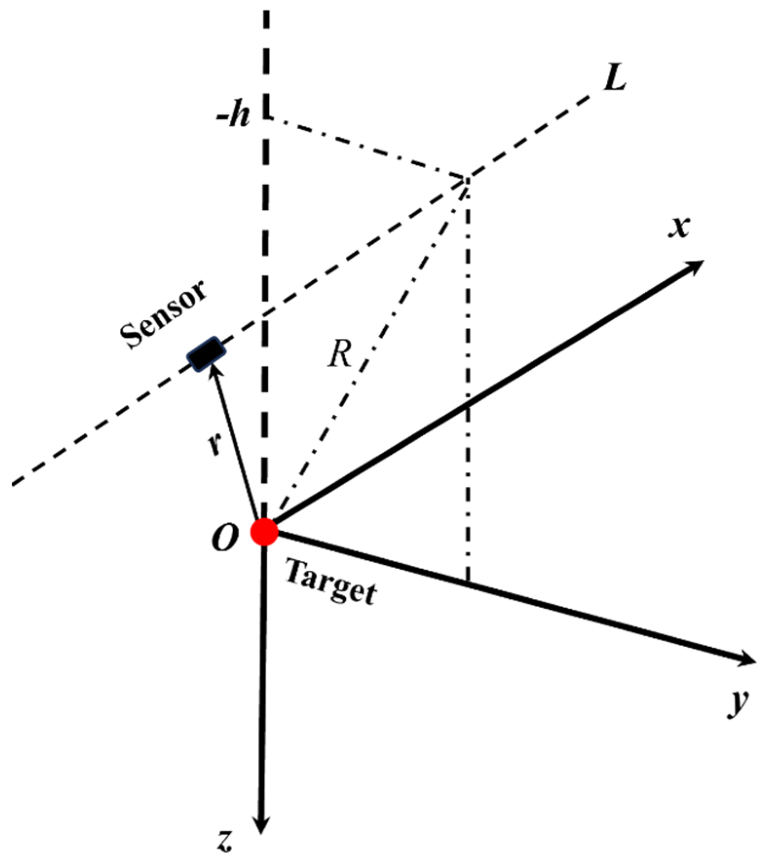
Figure 6.
Schematic of the search space for the target location.

Figure 7.
The distribution of the cost function with the position error of the target: (a) distribution of the cost function with the position error of the target in the xOy plane; (b) distribution of the cost function with the position error of the target in the xOz plane.
Figure 7.
The distribution of the cost function with the position error of the target: (a) distribution of the cost function with the position error of the target in the xOy plane; (b) distribution of the cost function with the position error of the target in the xOz plane.
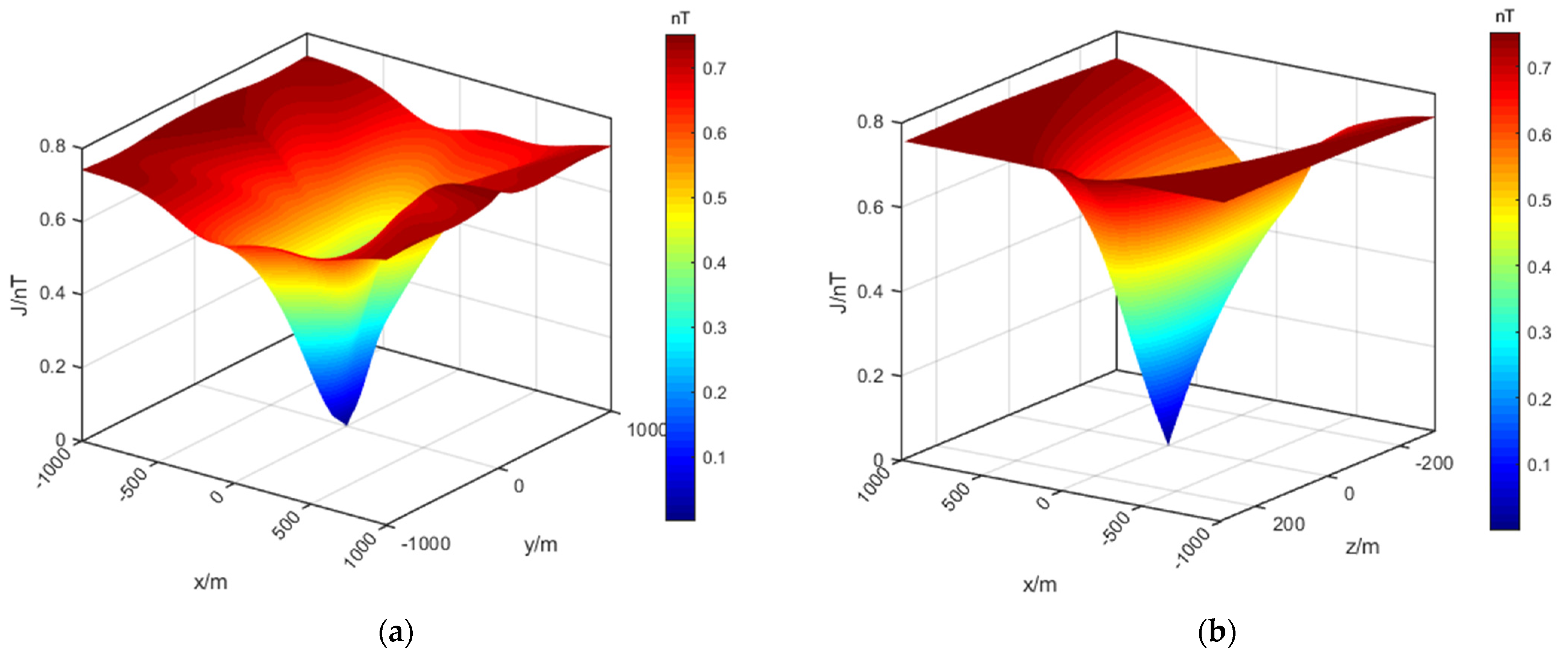
Figure 8.
Simulation of magnetic moment inversion for the typical targets: (a) magnetic moment magnitude; (b) magnetic moment inclination; (c) magnetic moment declination.
Figure 8.
Simulation of magnetic moment inversion for the typical targets: (a) magnetic moment magnitude; (b) magnetic moment inclination; (c) magnetic moment declination.
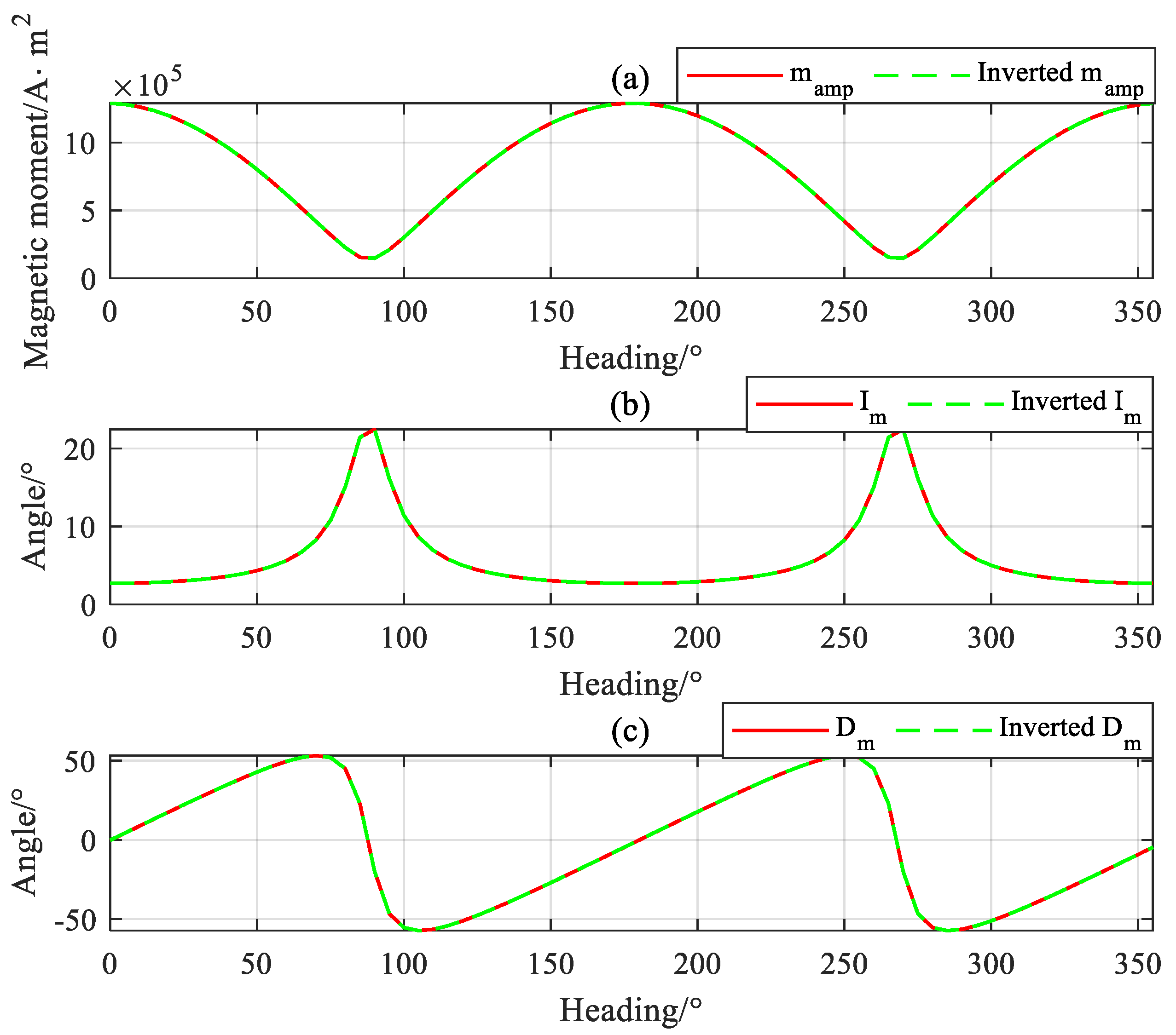
Figure 9.
Simulation of magnetic moment inversion errors for the typical target: (a) error of magnetic moment magnitude; (b) error of magnetic moment inclination; (c) error of magnetic moment declination.
Figure 9.
Simulation of magnetic moment inversion errors for the typical target: (a) error of magnetic moment magnitude; (b) error of magnetic moment inclination; (c) error of magnetic moment declination.
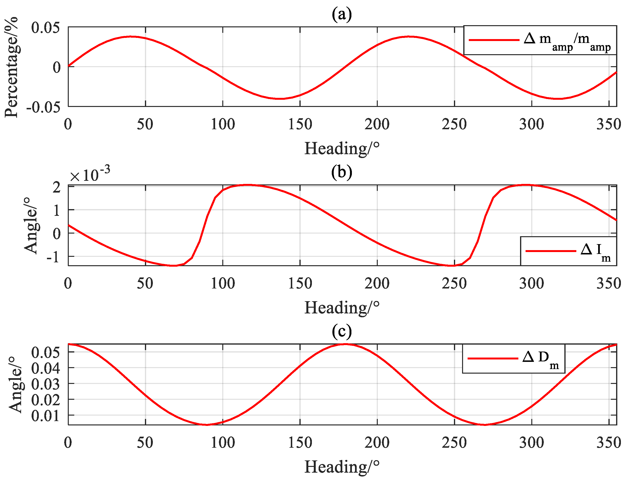
Figure 10.
Flow chart of noise reduction processing of aeromagnetic data.

Figure 11.
Experimental results of magnetic moment inversion for the typical target: (a) magnetic moment magnitude; (b) magnetic moment inclination; (c) magnetic moment declination.
Figure 11.
Experimental results of magnetic moment inversion for the typical target: (a) magnetic moment magnitude; (b) magnetic moment inclination; (c) magnetic moment declination.

Figure 12.
Errors in the magnetic moment inversion experiment: (a) error of magnetic moment magnitude; (b) error of magnetic moment inclination; (c) error of magnetic moment declination.
Figure 12.
Errors in the magnetic moment inversion experiment: (a) error of magnetic moment magnitude; (b) error of magnetic moment inclination; (c) error of magnetic moment declination.

Table 1.
Simulation results of magnetic moment inversion error.
| Inversion Errors | Value |
|---|---|
| Amplitude error | 0.025% |
| Inclination error | 0.0012° |
| Deflection error | 0.0284° |
Table 2.
Fluxgate magnetometer and optical pump magnetometer parameters.
| Technical Indicators | Parameters | |
|---|---|---|
| Magnetic Sensors | Fluxgate Magnetometer | Optical Pump Magnetometer |
| Measuring range | ±10,000 nT | 15,000 nT~105,000 nT |
| Noise level | ||
| Orthogonality error | 0.5° | \ |
| Absolute accuracy | 10 nT | 2.5 nT |
Table 3.
Magnetic moment inversion error.
| Inversion Errors | Value |
|---|---|
| Amplitude error | 5.85% |
| Inclination error | 1.58° |
| Deflection error | 2.79° |
Disclaimer/Publisher’s Note: The statements, opinions and data contained in all publications are solely those of the individual author(s) and contributor(s) and not of MDPI and/or the editor(s). MDPI and/or the editor(s) disclaim responsibility for any injury to people or property resulting from any ideas, methods, instructions or products referred to in the content. |
© 2023 by the authors. Licensee MDPI, Basel, Switzerland. This article is an open access article distributed under the terms and conditions of the Creative Commons Attribution (CC BY) license (https://creativecommons.org/licenses/by/4.0/).
Share and Cite
MDPI and ACS Style
Zhang, K.; You, X.; Liu, X.; Liu, J.; Zhu, W. Inversion of Target Magnetic Moments Based on Scalar Magnetic Anomaly Signals. Electronics 2023, 12, 4900. https://doi.org/10.3390/electronics12244900
AMA Style
Zhang K, You X, Liu X, Liu J, Zhu W. Inversion of Target Magnetic Moments Based on Scalar Magnetic Anomaly Signals. Electronics. 2023; 12(24):4900. https://doi.org/10.3390/electronics12244900
Chicago/Turabian StyleZhang, Ke, Xiuzhi You, Xiaodong Liu, Jiarui Liu, and Wanhua Zhu. 2023. "Inversion of Target Magnetic Moments Based on Scalar Magnetic Anomaly Signals" Electronics 12, no. 24: 4900. https://doi.org/10.3390/electronics12244900
Note that from the first issue of 2016, this journal uses article numbers instead of page numbers. See further details here.