Review

A Review for the Euler Number Computing Problem

1
Artificial Intelligence Institute, School of Electronic Information and Artificial Intelligence, Shaanxi University of Science and Technology, Xi’an 710021, China
2
School of Computer Science, Xianyang Normal University, Xianyang 712000, China
3
Faculty of Advanced Business, Nagoya Sangyo University, Owariasahi 4888711, Japan
4
School of Information Science and Technology, Aichi Prefectural University, Nagakute 4801198, Japan
*
Author to whom correspondence should be addressed.
Electronics 2023, 12(21), 4406; https://doi.org/10.3390/electronics12214406
Submission received: 31 August 2023 / Revised: 17 October 2023 / Accepted: 23 October 2023 / Published: 25 October 2023
(This article belongs to the Topic Computer Vision and Image Processing)

Abstract

:
In a binary image, the Euler number is a crucial topological feature that holds immense significance in image understanding and image analysis owing to its invariance under scaling, rotation, or any arbitrary rubber-sheet transformation of images. This paper focuses on the Euler number computing problem in a binary image. The state-of-the-art Euler number computing algorithms are reviewed, which obtain the Euler number through different techniques, such as definition, features of binary images, and special data structures representing forms of binary images, and we explain the main principles and strategies of the algorithms in detail. Afterwards, we present the experimental results to bring order of the prevailing Euler number computing algorithms in 8-connectivity cases. Then, we discuss both the parallel implementation and the hardware implementation of algorithms for calculating the Euler number and present the algorithm extension for 3D image Euler number computation. Lastly, we aim to outline forthcoming efforts concerning the computation of the Euler number.

1. Introduction

A digital binary image is formed by combining the planar connected areas that depict the projections of the objects present with the real-world scene being captured. Moreover, it can be considered a two-dimensional array with two possible results, i.e., 0 or 1. A connected region in a binary image is also called a connected component. It refers to the connected region composed of adjacent pixels with the same pixel value (usually object pixel) in a binary image. A hole in the image refers to the regions with non-object pixels surrounded by a connected component. By analyzing the pixels comprising each object presented in a binary image, it is possible to extract various topological and geometrical features that can be used to describe the properties or attributes of the objects. Examples of the features include area, perimeter, centroid, orientation, convexity, and Euler number. These features can be used for further analysis, classification, and recognition of objects within the image. Among the features, the Euler number, which can be obtained by subtracting the number of holes from the number of connected components (connected regions) in the given image, has been identified as a significant feature in many image analysis applications [1,2,3]. For example, we can calculate the Euler numbers if we need to distinguish the letter “A” and the letter “B” in a binary image. Obviously, the Euler number of the letter “A” is 0 and that of the letter “B” is −1; thus, we can distinguish them easily. The Euler number is also used in various mathematical models and methods for computer vision tasks [4,5,6].
In well-known digital image-processing textbooks [7,8], the notation p(x, y) is used for representing the pixel located at coordinate (x, y) in a binary image with a resolution of N × N pixels. The elements x and y in the coordinate (x, y) are integers between 0 and N − 1, both included. In situations where the meaning is unambiguous, p(x, y) can also be used to refer to its own value in image processing. In the context of binary images, pixels that are part of the object are considered foreground pixels, whereas pixels that are not part of the object are known as background pixels. Unless specified otherwise, it is generally assumed that the values of foreground pixels are represented by 1, whereas the values of background pixels are represented by 0. Moreover, to simplify matters, it is generally assumed that the pixels located on the borders of a binary image are background pixels, i.e., the value of all pixels on the borders of the given image is 0.
In a binary image, a pixel q is regarded as a 4-connectivity pixel of pixel p when they share a common edge. Alternatively, a pixel q is considered to be an 8-connectivity pixel of pixel p when they share a common edge or a common corner. As shown in Figure 1a, pixels q2, q4, q6, and q8 are 4-connectivity pixels of pixel p, and q1, q2, …, and q8 are 8-connectivity pixels of pixel p. Following this consideration, as shown Figure 1b, there are three connected components in the image in the case of 4-connectivity, but there is only one connected component in the case of 8-connectivity.
As described above, there are 4-connectivity cases and 8-connectivity cases between pixels, and, accordingly, we can calculate the Euler number in two cases, i.e., the 4-connectivity Euler number and the 8-connectivity Euler number. For example, as shown in Figure 2, in the case of 4-connectivity, there are three connected components and three holes; thus, the 4-connectivity Euler number is 3 − 3 = 0. However, in the case of 8-connectivity, only two connected components and three holes exist in Figure 2, so the Euler number is 2 − 3 = −1. Hereafter, whenever we refer to an “image,” we are actually referring to a binary image.
Although the Euler number is calculated by subtracting the number of holes from the number of connected components in an image, considering the complexity of obtaining the numbers of holes and connected components, many researchers have presented different kinds of algorithms by using the local information in an image when obtaining the Euler number over the past few decades. Based on the computing strategies, intrinsic features of images, data structure, and/or computer architecture being used, the Euler number computing algorithms can be divided into six categories:
(1)
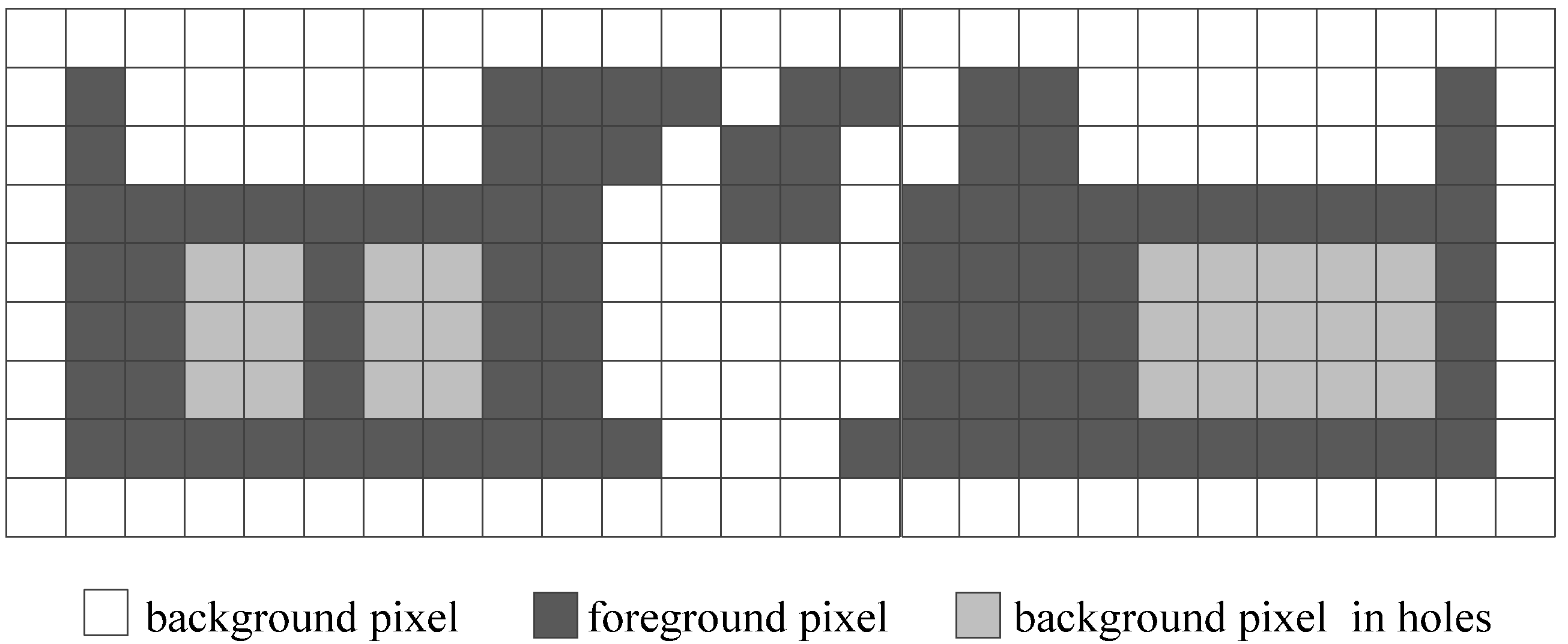
Algorithms that compute the Euler number by the definition in [9,10]. As described above, for a given image, the definition of the Euler number is the disparity between the numbers of connected components and holes. Thus, to compute the Euler number, these algorithms need to obtain the number of holes and the number of connected components in the given image. Accordingly, to achieve this goal, complicated labeling operations need to be conducted to distinguish every connected component and every hole in the image. Once the number of holes and connected components is acquired, we can obtain the Euler number easily.
(2)
Algorithms that compute the Euler number by utilizing the intrinsic features of the image [11,12,13,14,15,16]. In these algorithms, different features of an image are used to calculate the Euler number. For example, taking advantages of the skeleton, the perimeter/contact perimeter and the special contour pixels of the image, we can compute the Euler number in different ways.
(3)
Algorithms that compute the Euler number by counting specific blocks/patterns in the image [17,18,19,20,21,22,23,24,25]. In these algorithms, specific patterns with 2 × 2 pixels and consecutive foreground pixel blocks in the same row in the image, called runs, can be employed for calculating the Euler number. Moreover, using a raster scan, these algorithms can be easily implemented in practice.
(4)
Algorithms that compute the Euler number with a special data structure [26,27,28,29,30,31,32,33]. Trees and graphs are special data structures for representing an image. By representing an image as a tree or a graph, these algorithms can compute the Euler number through the theorems or conclusions in the data structure of the tree or graph.
(5)
Algorithms that compute the Euler number using machine learning methods [34,35,36]. In the past decade, machine learning/deep learning methods have been widely adopted for image classification and image recognition tasks. Then, some researchers have adopted these methods for Euler number computation. Experimental results have verified the accuracy of these methods in Euler number computation. However, these methods need to collect a lot of samples and take a long time to train the samples. Therefore, for only obtaining the Euler number, these methods may not be so efficient.
(6)
Algorithms that compute the Euler number using special structure computers [37,38,39,40,41,42]. As mentioned in Class (3), the Euler number can be determined by identifying specific patterns within the raster scan and counting them. Then, VLSI (very large-scale integration), co-processor, and pipeline architecture can be employed for counting these patterns within different regions of a given image simultaneously to improve the conventional algorithms.
Considering that algorithms for ordinary computer architectures in Class (1)–Class (4) are the base of algorithms in Class (6), we will not discuss the Euler number computing algorithms in Class (6) in this paper. Moreover, the Euler number is seldom computed with the algorithms mentioned in Class (5) in practice; thus, we will primarily concentrate on the algorithms belonging to Class (1), (2), (3), and (4) in this paper.
This paper provides a review of strategies for Euler number computing algorithms. Additionally, experimental results will be presented to bring order to the classical algorithms. The state-of-the-art algorithms are of particular focus in this paper, which are listed as follows:
(a)
Algorithm that computes the Euler number with the definition proposed in Ref. [9];
(b)
Algorithm that computes the Euler number with the skeleton of a given image, as proposed in Ref. [11];
(c)
Algorithm that computes the Euler number via the perimeter of connected components in a given image, as proposed in Ref. [12];
(d)
Algorithm that computes the Euler number via corner codification of foreground pixels in a given image, as proposed in Ref. [16];
(e)
Algorithm that computes the Euler number via specific 2 × 2 bit-quad patterns in a given image, as proposed in Ref. [17];
(f)
Algorithm that computes the Euler number via runs in a given image, as proposed in Ref. [23];
(g)
Algorithm that computes the Euler number by representing a given image as a graph, as proposed in Ref. [27];
(h)
Algorithm that computes the Euler number by representing a given image as a tree, as proposed in Ref. [31];
(i)
Algorithm that computes the Euler number via graph representation of specific runs in a given image, as proposed in Ref. [33].
Among the above algorithms, the algorithm mentioned in (a) calculates the Euler number according to the definition, the algorithms mentioned in (b)–(d) calculate the Euler number by making use of a given image’s intrinsic features, the algorithms mentioned in (e)–(f) calculate the Euler number by counting specific patterns in a given image, and the others obtain the Euler number by representing an image as a special data structure.
In the past few decades, different Euler number computing algorithms have been illustrated in various studies, as listed above, by using different local information in images. These studies focused on describing their proposed methods, without elaborating on other state-of-the-art methods and lacking a comparison of experimental results among different methods. This paper focuses on the state-of-the-art Euler number computing algorithms. We review different kinds of Euler number computing algorithms and explain the main principles and strategies of the algorithms in detail. Moreover, we present the experimental results to bring order of the prevailing Euler number computing algorithms in 8-connectivity cases.
The subsequent sections of this paper are structured in the following manner: We review and describe the strategies of state-of-the-art Euler number computing algorithms in the next section. In Section 3, we present a comparison of the algorithms and the experimental results of the comparison for different kinds of images. In Section 4, we cover concerns related to hardware and parallel implementation of Euler number computation and bring an extension of Euler number computing algorithms for 3D images. Lastly, Section 5 contains our concluding remarks and outlines the next study focuses.

2. Reviews of State-of-the-Art Euler Number Computing Algorithms

2.1. Algorithms That Compute the Euler Number through the Definition

As described in Ref. [7], the Euler number can be obtained by subtracting the number of holes from the number of connected components in an image. Obviously, to obtain the Euler number, the most direct method is to count the number of connected components and holes in an image. Then, it can be obtained easily by using Formula (1).
E = CH
Here, C refers to the number of connected components, whereas H represents the number of holes in the image.
As we know, connected component labeling (CCL) algorithms are classical and efficient algorithms for distinguishing the different objects in an image, and they can be employed for labeling and calculating the holes and the connected components simultaneously. When the labeling process is completed, every foreground/background pixel is assigned a unique label, so the foreground (or background) pixels px and py have the same label if and only if they are in the same connected component/hole. Then, we can calculate the number of connected components and holes by counting the different labels, and thus, Formula (1) can be used for calculating the Euler number.
In Ref. [9], He et al. presented an efficient labeling algorithm for distinguishing the different connected components and different holes and computing the Euler number of an image. In the proposed algorithm, the connected components are labeled in the case of 8-connectivity and the holes are labeled in the case of 4-connectivity (otherwise, if the holes are also labeled in the case of 8-connectivity, there will be no holes existing in the given image); thus, this algorithm computes the 8-connectivity Euler number in practice.
To achieve the above goal, this algorithm extends the labeling strategy proposed in Ref. [10], which needs to scan the image forward twice and conduct three phases.
Phase 1: Label assigning. The algorithm assigns temporary labels to the pixels of the image, which can either be a new label or an existing one that has already been assigned to the labeled pixels.
Phase 2: Label recording and resolving. When Phase 1 is completed, each pixel is assigned a temporary label. In fact, some different labels may belong to the same connected component/hole, and they are considered to be in the same equivalent class; therefore, the algorithm needs to record and resolve these equivalent labels.
Phase 3: Label replacing. Lastly, the algorithm replaces every temporary label with a representative label. After the algorithm has done this, all pixels in the same connected component and all pixels in the same hole will have a unique label. Accordingly, we can count the different labels to obtain the number of holes and connected components.
To complete the above three phases, the algorithm needs to conduct two raster scans of the image. In the first scan, the designed working mask presented in Figure 3a is used to label the connected components and comprises four scanned neighboring pixels of the processing foreground pixel. Moreover, this working mask is also used to assign or share a temporary label for every foreground pixel and to record the labels and resolve equivalent label classes of the connected components. At the same time, the working mask, shown in Figure 3b, is used to label the holes, which comprise two scanned neighboring pixels of the processing background pixel. The same steps are carried out to process each foreground pixel. This working mask is also used to assign or share a temporary label for each background pixel and to record the labels and resolve equivalent label classes of the holes. At all times, equivalent temporary labels are grouped together in an equivalent set with the same representative label.
As illustrated in Figure 3a, when processing the foreground pixel p(x, y), four pixels—p(x − 1, y), p(x − 1, y − 1), p(x, y − 1), and p(x + 1, y − 1)—in the working mask need to be accessed. If there is no foreground pixel in the working mask, it can be concluded that the processing pixel will not connect to any processed foreground pixel. In other words, the processing pixel should belong to a new connected component. Consequently, a new temporary label should be assigned to the current pixel. Otherwise, if there are some foreground pixels in the working mask, the processing pixel and the foreground pixels that already exist should be part of the same connected component. In this case, any of the labels in the working mask can be assigned to the current pixel.
When labeling the holes, for the processing background pixel p(x, y), if there is no background pixel in the working mask, i.e., if both p(x − 1, y) and p(x, y − 1) are foreground pixels, it can be concluded that no processed background pixels are connected to the background pixel currently being processed and that the processing pixel should belong to a new hole. Thus, a new temporary label should be assigned to the processing background pixel. Otherwise, if some background pixels exist in the working mask, the processing background pixel and the existing background pixels should belong to the same hole. Then, the processing background pixel should be assigned any of the labels in the working mask.
All temporary labels that belong to the same connected component or the same hole will be merged into a set of equivalent labels when the first scan is completed. In the second raster scan, by replacing each temporary label with the corresponding representative label, it will assign unique labels to all foreground pixels within each connected component and to all background pixels within each hole. Hence, to obtain the number of connected components and holes, the algorithm only needs to count the different labels. Lastly, the image’s Euler number can be obtained simply by using Formula (1). We refer to the labeling-based algorithm as the LB algorithm for simplicity in this paper.
Obviously, for labeling the connected components and holes of an image, we need to have a comprehensive perspective of the whole image. At the same time, the labeling procedure is very complicated in terms of recording and resolving the equivalent labels. Although the number of holes and connected components can be obtained simultaneously by this algorithm, it is not the best choice for obtaining the Euler number only.

2.2. Algorithms That Compute the Euler Number by Utilizing Intrinsic Features

Some intrinsic features, such as the skeleton, can preserve important topological information of an image. Hence, instead of counting connected components and holes in a given image directly, the Euler number can be computed with the perimeters of objects and special pixels in the skeleton of the image.

2.2.1. Skeleton-Based Euler Number Computing Algorithm

The skeleton of an image can maintain the connectivity of small parts of the image, which helps to highlight object features and reduce redundant information. Moreover, it can preserve some useful topological features, such as the number of holes and connected components. Accordingly, researchers have proposed some algorithms for obtaining the Euler number by utilizing the skeleton of a given image.
Ref. [11] presented a skeleton-based 4-connectivity Euler number computing algorithm that computes the Euler number of a given image by using the number of terminal pixels and three-edge pixels in the skeletonized image. To do this, it needs to calculate the number of neighboring pixels in a foreground pixel p, which is denoted as Nc(p). Nc(p) is different than 0. As is defined in Ref. [11]:
(1)
If Nc(p) = 1, pixel p is called a terminal pixel (Tp);
(2)
If Nc(p) = 2, pixel p is called an internal pixel;
(3)
If Nc(p) = 3, pixel p is called a three-edge pixel (TEp);
(4)
If Nc(p) > 3, pixel p is called a crossing pixel.
Once the number of terminal pixels and three-edge pixels is obtained, we can calculate the Euler number by using Formula (2).
E = T p s T E p s 2
Here, Tps is the number of terminal pixels, whereas TEps is the number of three-edge pixels in the skeletonized image.
Moreover, if there is a crossing pixel in the skeletonized image, it needs to be decomposed into two three-edge pixels (TEps). For example, as shown in Figure 4a, pixel p1 and pixel p3 are three-edge points, and pixel p2 is a crossing point, which should be decomposed into two three-edge points (as shown in Figure 4b). Moreover, pixels p4, p5, p6, and p7 are terminal pixels. According to Formula (2), the Euler number is E = (TpsTEps)/2 = (4 − 4)/2 = 0. In fact, there is one connected component and one hole in Figure 4a, so the Euler number is E = CH = 1 − 1 = 0 according to the definition, which is consistent with the result calculated with Formula (2).
Although the computing formula is very simple in the skeleton-based Euler number computing algorithm, it is necessary to skeletonize the given image in advance, which will influence the efficiency of the algorithm to a certain extent. Furthermore, there are two special cases, i.e., when only one pixel or loop is contained in the image, in which this algorithm cannot compute Euler number correctly.

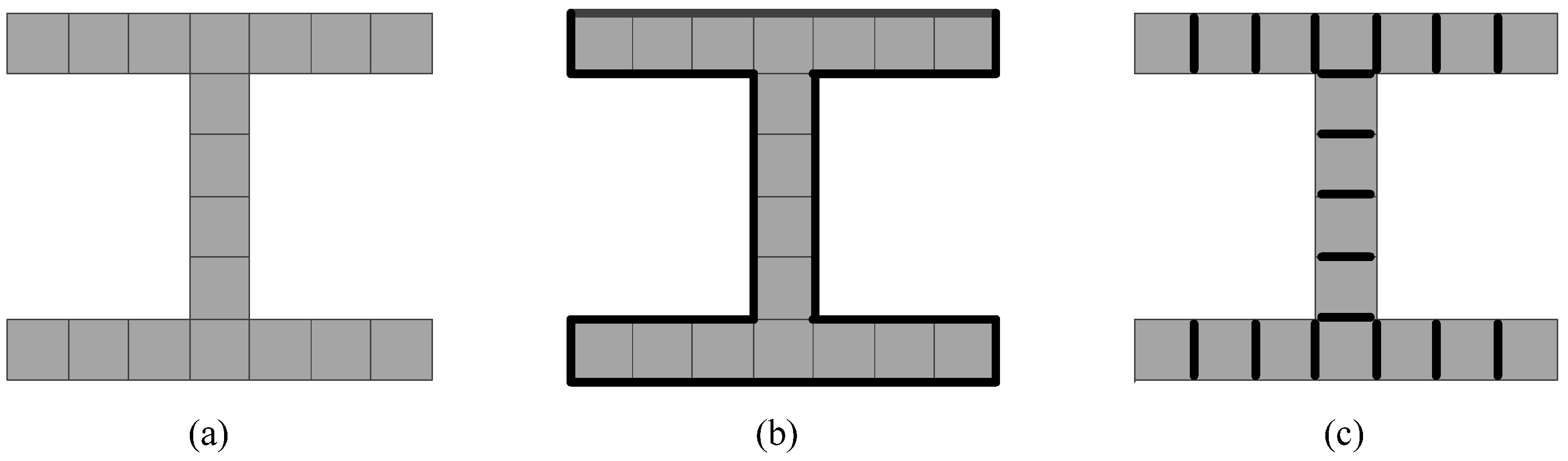
2.2.2. Perimeter-Based Euler Number Computing Algorithm

Besides employing the skeleton of a given image, Bribiesca used the perimeter and contact perimeter of the connected components (or shapes) to compute the 4-connectivity Euler number in Ref. [12]. The related definition of the perimeter and contact perimeter can be found in Ref. [13]. Furthermore, this method is only suitable for one-pixel-width images, with one connected component in the images.
The perimeter P refers to the boundary length of a connected component in an image, which is determined by adding up the total lengths of the sides of the pixels making up the connected component. This is in accordance with the traditional definition of a perimeter. For example, Figure 5a presents an instance of a connected component comprising 18 pixels, and Figure 5b illustrates the perimeter of the connected component presented in Figure 5a, which is marked by bold lines. The contact perimeter of an image is denoted as Pc, which is comprised of pixels corresponding to the total length of the segments shared by the neighboring pixels. Figure 5c illustrates the contact perimeter of Figure 5a, which is also marked by bold lines.
When obtaining the perimeter and contact perimeter, we can compute the Euler number by using Formula (3).
E = P P c ( T 2 ) T
In Formula (3), the number of sides of a pixel is denoted as T, and for the case of the rectangular pixels in the image, T = 4.
For the image shown in Figure 5a, the perimeter P is 38, the contact perimeter Pc is 17, and T is 4. According to Formula (3), the Euler number is E = (PPc (T − 2))/T = (38 − 34)/4 = 1.
However, the method suggested in Ref. [12] cannot calculate the Euler number correctly when the given image is not composed of one connected component or it is not a one-pixel-width image. As an improvement, Sossa [14,15] presented other methods for obtaining the Euler number by using the perimeter and contact perimeter of the image, which can compute it for a non-one-pixel-width image with more than one connected component correctly. To obtain the Euler number according to the algorithm presented by Sossa, the image needs to be eroded by a 2 × 2 structural element, shown in Figure 6a, in advance, and the pixels remaining as a result of the erosion are called “tetra pixels”.
As shown in Figure 6b, if the image is eroded by the structural element, only two tetra pixels remain as a result, as shown in Figure 6c. In fact, if an image is one pixel width, there will be no tetra pixels after erosion; conversely, if there is at least one tetra pixel in the image after erosion, it is not a one-pixel-width image. Let NT denote the number of tetra pixels remaining after the erosion operation. We can compute the Euler number by using Formula (4).
E = N T P c ( T 2 ) P T
In fact, the number of tetra pixels remaining after the erosion operation is equal to the number of 2 × 2 foreground pixel patterns in the image, and this can be calculated by a simple raster scanning of the image. In Figure 6b, the perimeter and contact perimeter are 34 and 25, respectively. Moreover, there are two 2 × 2 foreground pixel patterns; thus, NT should be 2. According to Formula (4), the Euler number is computed as E = NT − (Pc (T − 2) − P)/T = 2 − (50 − 34)/4 = −2.
In Figure 6b, there are three holes and one connected component. Based on the definition of the Euler number, it is E = CH = 1 − 3 = −2, which is consistent with the result calculated with Formula (4).

2.2.3. Corner Codification-Based Euler Number Computing Algorithm

The contour pixel information in an image is very useful for image analysis and understanding. Accordingly, Ref. [16] proposed a 4-connectivity corner codification-based algorithm for computing the Euler number, taking advantage of the number of foreground pixels that each connected component’s exterior contour pixels contacts.
According to the proposed algorithm, every exterior contour pixel that touches the connected component’s background directly will be encoded by the number of foreground pixels it touches. As shown in Figure 7a, there are four corners in a foreground pixel, i.e., NW, NE, SW, and SE. Moreover, there are only three codifications for the corners of exterior contour pixels, i.e., 1, 2, and 3. For example, for the contour pixel a in Figure 7a:
(1)
The NW corner touches one foreground pixel, i.e., pixel a; thus, the codification of this corner is 1.
(2)
The NE corner touches two foreground pixels, i.e., pixel a and pixel b; thus, the codification of this corner is 2.
(3)
The SW corner touches three foreground pixels, i.e., pixel a, pixel c, and pixel d; thus, the codification of this corner is 3.
(4)
The SE corner touches three foreground pixels, i.e., pixel a, pixel b, and pixel d; thus, the codification of this corner is 3.
Let N1 be the number of corners whose corner codifications are 1, and let N3 be the number of corners whose corner codifications are 3. The image’s Euler number can be obtained by using Formula (5).
E = N 1 N 3 4
For example, as shown in Figure 7b, there are 18 corners whose codifications are 1 and 18 corners whose codifications are 3. According to Formula (5), the Euler number is E = (N1N3) = (18 − 18)/4 = 0.
In fact, there is one connected component and one hole in Figure 7b, so the Euler number is E = CH = 1 − 1 = 0 according to the definition, which is consistent with the result calculated with Formula (5). Then, when the image is transformed into the one in Figure 7c, both N1 and N3 are 16 and the Euler number of the image is still 0. It is verified that the Euler number remains unchanged when the image is transformed or rotated.

2.3. Algorithms That Compute the Euler Number by Counting Specific Blocks/Patterns in the Image

In Ref. [24], Lin proved that Euler number computation satisfies the additive theorem. In other words, to obtain the Euler number, we can independently calculate the Euler number of a small portion of a given image and summarize all of the results to obtain the image’s Euler number. Hence, different from the method described in Ref. [9], the Euler number can be obtained without a comprehensive understanding of the image in advance.

2.3.1. Bit-Quad-Based Euler Number Computing Algorithm

In Ref. [17], a classical and efficient algorithm is presented for Euler number computation. This algorithm computes the Euler number by counting specific bit-quads in an image composed of 2 × 2 pixels. Because this algorithm is very easy to implement, the widely recognized commercial image-processing software MATLAB R2018b has incorporated this algorithm [18]. For convenience, this classical bit-quad-based algorithm is represented as the C-BQ algorithm in this paper.
The C-BQ algorithm [17] computes the Euler number by counting specific bit-quads in an image. To implement the algorithm, it is necessary to conduct a raster scan of the image horizontally from left to right and vertically from top to bottom. For every pixel p(x, y) accessed in the raster scan, four pixels should be accessed in the corresponding bit-quad [ p ( x , y ) p ( x + 1 , y ) p ( x , y + 1 ) p ( x + 1 , y + 1 ) ] to confirm whether the current bit-quad exists in patterns Pat1, Pat2, or Pat3, as shown in Figure 8.
Let NP1, NP2, and NP3 denote the number of patterns Pat1, Pat2, and Pat3 that occurred in the image, respectively. Then, the 4-connectivity Euler number can be computed by using Formula (6), whereas for 8-connectivity cases, the computing formula is Formula (7).
E 4 = N P 1 N P 2 + 2 N P 3 4
E 8 = N P 1 N P 2 2 N P 3 4
It is obvious that, to compute the Euler number with the C-BQ algorithm, we scan the image, access the pixels, check the corresponding bit-quads, and confirm whether they should be counted or not. For each scanned pixel, we have to access the other three neighboring pixels in the corresponding bit-quad. As a result, we need to access four pixels when processing each pixel in the C-BQ algorithm. For an image with a resolution of X × Y pixels, while computing its Euler number, we have to access 4 × X × Y pixels in the C-BQ algorithm.
However, some pixels are accessed redundantly during the computation procedure with the C-BQ algorithm. For example, as shown in Figure 9, when we process pixel p11, we need to access pixels p11, p12, p21, and p22 in the corresponding bit-quad [ p 11 p 12 p 21 p 22 ] to confirm whether this bit-quad should be counted or not. Then, when we process the next pixel, p12, in the same row, we need to access pixels p12, p13, p22, and p23 in the corresponding bit-quad [ p 12 p 13 p 22 p 23 ] to confirm whether this bit-quad should be counted or not. Obviously, pixels p12 and p22 were already accessed while processing pixel p11. On the other hand, when we process pixel p21 in the next row, we need to access pixels p21, p22, p31, and p32 in the corresponding bit-quad [ p 21 p 22 p 31 p 32 ] . It is found that pixels p21 and p22 were also accessed while processing pixel p11.
In order to avoid accessing pixels repeatedly while processing pixels in the raster scan, Yao et al. [19,20] proposed two efficient strategies, i.e., state transition and multi-row scanning, to reduce redundant pixel access from the horizontal direction and vertical direction of the image.
  • Strategy of state transition
As described above, two pixels are accessed repeatedly while processing the current pixel and the previous pixel in the same row in the C-BQ algorithm. In fact, the repeated access can be avoided by use of the values acquired while processing the previous pixel. As shown in Figure 10, in order to represent the values of the two accessed pixels, four states, St1St4, are defined in Ref. [19], and, taking advantage of transitions among the states, only two pixels need to be accessed to process a pixel.
In implementation, based on the prior assumption that all pixels on the border are background pixels, the algorithm begins the processing from St1, and it only needs to access two pixels on the right of the bit-quad, i.e., px and py in Figure 10, to confirm whether the current bit-quad should be counted or not. According to the values of pixel px and pixel py, the next bit-quad to be checked must be one of the four states, and to confirm whether the next bit-quad should be counted or not, still only two pixels need to be accessed. In other words, following the strategy of state transition, only the right two pixels need to be accessed in a bit-quad to confirm whether the current bit-quad should be counted or not. Therefore, the number of pixels that need to be accessed to process a pixel can decrease from four to two. That is to say, we only need to access 2 × X × Y pixels to compute the Euler number of an X × Y-size image with this strategy.
Hence, the problem of accessing pixels repeatedly from the horizontal direction of an image can be solved via the strategy of state transition. To simplify matters, the algorithm introduced in Ref. [19] is denoted as the IH-BQ algorithm.
2.
Strategy of multi-row scanning
In the IH-BQ algorithm, by using the four defined states, only two pixels need to be accessed to process a pixel in an image. However, there are pixels that are accessed repeatedly when processing pixel p(x, y) and pixel p(x, y + 1) in the next row. For example, we need to check the corresponding bit-quad [ p ( x , y ) p ( x + 1 , y ) p ( x , y + 1 ) p ( x + 1 , y + 1 ) ] to confirm whether it should be counted or not when processing pixel p(x, y). While processing pixel p(x, y + 1) in the next row, we have to check the corresponding bit-quad [ p ( x , y + 1 ) p ( x + 1 , y + 1 ) p ( x , y + 2 ) p ( x + 1 , y + 2 ) ] . Then, it is noticed that pixel p(x, y + 1) and pixel p(x + 1, y + 1) are accessed repeatedly.
In order to avoid the repeated access of pixels mentioned above, Ref. [20] presented an efficient strategy that scans image rows two by two. For example, when processing pixel p(x, y), we access six pixels [ p ( x , y ) p ( x + 1 , y ) p ( x , y + 1 ) p ( x + 1 , y + 1 ) p ( x , y + 2 ) p ( x + 1 , y + 2 ) ] once and confirm whether the two bit-quads [ p ( x , y ) p ( x + 1 , y ) p ( x , y + 1 ) p ( x + 1 , y + 1 ) ] and [ p ( x , y + 1 ) p ( x + 1 , y + 1 ) p ( x , y + 2 ) p ( x + 1 , y + 2 ) ] should be counted or not. Via this means, we need to access 6/2 = 3 pixels to process a bit-quad, which seems to be more than with the IH-BQ algorithm.
If the two strategies of state transition and multi-row scanning can be employed simultaneously, we can check two bit-quads by accessing three pixels. In other words, 3/2 = 1.5 pixels need to be accessed to process a bit-quad, which is fewer than with the IH-BQ algorithm, and then, the efficiency of algorithm can be improved further.
Following this consideration, when every row n of the given image is scanned, we can confirm whether n bit-quads should be counted or not by accessing n + 1 pixels. Then, (n + 1)/n pixels need to be accessed to process each bit-quad on average. Theoretically, as the ever-increasing number of bit-quads is simultaneously processed, the average number of pixels that need to be accessed to process each bit-quad will decrease. At the same time, the algorithm will become more complex as the number of bit-quads being processed simultaneously increases, and it may not be very efficient in practice. Ref. [20] studied the bit-quad-based algorithms and implemented the algorithm of multi-row scanning every three rows, every four rows, and every five rows and verified that the best compromise for this algorithm is to scan five rows once and process four bit-quads simultaneously. To simplify matters, we denote the algorithm presented in Ref. [20] as the I-BQ algorithm.
Furthermore, to obtain the Euler number, Gomez [21] and Sossa [22] presented alternative formulas by use of bit-quads. Similar to the C-BQ algorithm, there are pixels that are accessed repeatedly upon implementation, and the proposed algorithm can be improved by using the strategies of state transition and multi-row scanning.

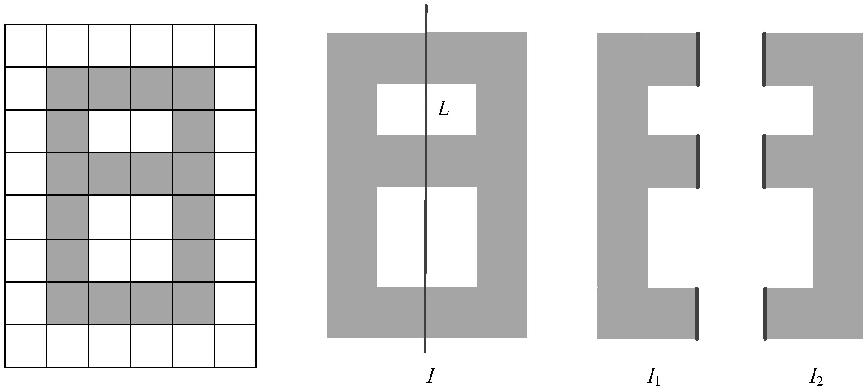
2.3.2. Run-Based Euler Number Computing Algorithm

Besides certain 2 × 2 bit-quad patterns, the Euler number can be obtained based on the consecutive foreground pixel patterns, called runs, in each row in an image. Ref. [23] suggested an algorithm for obtaining the 8-connectivity Euler number by using the number of runs and 8-connectivity runs in an image.
If there is a pixel p1 in run R1 of a row and a pixel p2 in run R2 of another adjacent row such that they are 8-connectivity, then runs R1 and R2 are considered to be 8-connectivity.
As shown in Figure 11, the number of runs in the second row, the third row, the fourth row, and the fifth row are two, four, four, and one, respectively. Moreover, there are 15 8-connectivity runs in the adjacent rows, which are marked by oval shapes. It is noticed that a run can be an 8-connectivity run of other runs in adjacent rows simultaneously.
According to the above definition, the algorithm [23] computes the Euler number by using the difference between the runs and the 8-connectivity runs in the image. The correctness of this algorithm is proven by using the additive theorem [24]. Let RUNS and NBRUNS denote the numbers of runs and 8-connectivity runs, respectively. We can calculate the Euler number of an image by using Formula (8).
E = RUNS − NBRUNS
As a result, for the image shown in Figure 11, the Euler number is E = RUNSNBRUNS = (2 + 4 + 4 + 1) − 15 = −4. In fact, only one connected component exists in the image in the case of 8-connectivity. On the other hand, five holes labeled by the numbers 1, 2, 3, 4, and 5 are formed in the image. The Euler number is E = CH = 1 − 5 = −4, which is consistent with the result calculated with Formula (8). To simplify matters, this classical run-based algorithm is denoted as the C-RB algorithm in this paper.
Based on the description above, a raster scan should also be conducted on the given image with the C-RB algorithm for Euler number computation. For all scanned rows except the first row, we need to identify the shift from background pixel to foreground pixel to count the runs in each row. Meanwhile, the location information needs to be recorded to find the 8-connectivity runs between the current row and the previous row. When the last row is scanned completely, the numbers of runs and 8-connectivity runs can be obtained, and the Euler number can be calculated with Formula (8) easily.
As an improvement, based on the numbers of runs and 8-connectivity runs in the image, Ref. [25] presented another Euler number computing algorithm. Instead of processing rows of the image one by one from the first row to the last row, the improved algorithm divides the scanning procedure into two steps. In the first step, it scans the odd rows from the first row of the image, detects and counts the runs in the odd rows, and records the end locations. In the second step, it scans the even rows and detects and counts the runs in the even rows. At the same time, it also finds 8-connectivity runs formed in the previous row and the next row at once. To simplify matters, the algorithm mentioned in Ref. [25] is denoted as the I-RB algorithm in this paper.
Through in-depth analysis of the C-RB algorithm and the I-RB algorithm, we realized that all runs and all 8-connectivity runs need to be found in the two algorithms. On the other hand, both the start location and the end location need to be recorded in the C-RB algorithm, whereas only the end location needs to be recorded in the I-RB algorithm. Furthermore, all runs in a given image need to be recorded in the C-RB algorithm, whereas only runs in the odd rows need to be recorded in the I-RB algorithm, which can indicate an improvement over the C-RB algorithm.

2.4. Algorithms That Compute the Euler Number by Special Data Structure

Although images and graphs are stored differently in the memory of computers, there is still some connection between images and graphs [26,27,28]. When an image is represented by a graph, some useful conclusions and theorems in graph theory can be employed for image-processing tasks.

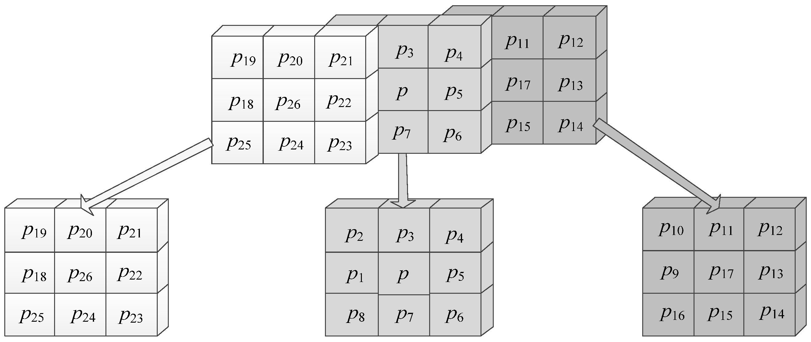
2.4.1. Graph-Representing-Based Euler Number Computing Algorithm

In Ref. [26], Chen presented a graph-representing-based algorithm for computing the 4-connectivity Euler number by employing the Euler formula, which is often used in graph theory.
To take advantage of the Euler formula in graph theory, an image needs to be represented by a graph. Because the images we processed are two-dimensional images, the corresponding graphs will be square graphs. To construct the graph, an image X is considered to be a subset in Z2, and every foreground pixel in the given image will be treated as a node. For any foreground pixel xi, xjX, add an edge eij between xi and xj if xi and xj are 4-connectivity. Wherever a 2 × 2 foreground pixel pattern [ 1 1 1 1 ] occurs in the image, there will be a basic face in the corresponding graph. When all foreground pixels are added to the graph and all edges and all basic faces are fully considered, we can construct a square graph. Denoting the numbers of nodes, edges, and basic faces as n, e, and f in the graph, respectively, the Euler number can be obtained by using Formula (9).
E = ne + f
Upon implementation, instead of constructing the corresponding graph in advance and counting the nodes, edges, and basic faces in the constructed graph, we can calculate them directly by using the given image. According to the graph-constructing rules, the number of nodes in the graph will be the same as that of the foreground pixels in the image. As for the edges, whenever there are two consecutive foreground pixels in the horizontal direction or the vertical direction of the image, there will be an edge. Thus, to calculate the number of edges, we should consider the configurations of [ 1 1 ] and [ 1 1 ] in the image. Lastly, while computing the basic faces, we only need to count the 2 × 2 foreground bit-quads in the given image, i.e., we only need to consider the configuration of [ 1 1 1 1 ] in the image.
For example, for the image shown in Figure 12, the number of nodes, edges, and basic faces is 15, 16, and 2, respectively; therefore, the Euler number is calculated as E = ne + f = 15 − 16 + 2 = 1. In fact, there are two connected components and one hole in the image, so the Euler number is E = CH = 2 − 1 = 1, according to the definition, which is consistent with the result calculated with Formula (9).
The algorithm presented in Ref. [26] calculates the 4-connectivity Euler number of an image according to the number of nodes, edges, and basic faces in the constructed graph corresponding to the image. Then, some researchers extended it to 8-connectivity and proposed some improvements in Refs. [27,28].
As shown in Figure 13, for the given image, when we take all foreground pixels as nodes and add all edges between two foreground pixels if and only if they are 8-connectivity neighbors, unless the resulting edge would cross another edge, we can construct a graph corresponding to the given image in the case of 8-connectivity. Obviously, the constructed graph is also a square graph. If we denote the number of nodes, edges, squares, and connected components in the graph as n, e, r, and C, respectively, we can obtain ne + r = C + 1 by using the Euler formula in graph theory.
In the Euler formula in graph theory, in an infinite square outside of the graph, all of the basic faces and holes can be treated as squares. Let H denote the number of holes and f denote the number of basic faces in the graph; the squares r are H + f + 1. By using the Euler formula, we can obtain ne + (H + f + 1) = C + 1. Therefore, we can calculate the Euler number as:
E = CH = ne + f
It looks the same as Formula (9). In other words, the image’s Euler number can be computed according to the number of nodes, edges, and basic faces in the corresponding graph in the case of 8-connectivity. However, it is noticed that the basic faces are referred to as right-angled triangle faces in the case of 8-connectivity.
Similarly, as in the algorithm presented in [26], the number of nodes, edges, and basic faces can be obtained by accessing all pixels in the given image without constructing a square graph in advance.
When implementing the algorithm, the number of nodes is the same as the number of foreground pixels in the image, which is the same as in the algorithm presented in [26]. According to the constructing rules, an edge should be added if and only if two foreground pixels are 8-connectivity neighbors and the added edge will not cross another edge in order to avoid calculating the edges repeatedly. To calculate the edges, the pixels in the image need to be accessed and whether two neighboring pixels can form a new edge or not needs to be determined. This procedure can be implemented by checking every bit-quad in the image. As shown in Figure 14, for each processing bit-quad, we access the pixels and calculate the edges marked by the dotted line. Noticed that if edges (p(x, y), p(x − 1, y-1)) and (p(x − 1, y), p(x, y − 1)) exist, only one edge will be counted because an edge should not cross with another edge.
When counting the basic faces, i.e., the right-angled triangle faces, all of the pixels in a bit-quad need to be accessed. If all of the pixels in a bit-quad are foreground pixels, two basic faces (right-angled triangle faces) will be formed in the graph. If there are three pixels in a bit-quad, only one basic face will be formed in the graph. Otherwise, no basic faces will be formed.
When all bit-quads in the image are processed, the number of nodes, edges, and basic faces can be obtained, and therefore, the Euler number can be easily calculated by using Formula (10).
Obviously, to reduce the complexity of the graph-representing-based Euler number computing algorithm, the procedure of calculating nodes, edges, and basic faces is converted to process the bit-quads in an image. Yao et al. [29] analyzed the configurations of each type of bit-quad; listed the increments in nodes, edges, and basic faces; and presented their Euler number increments, as shown in Table 1. It is obvious that only three types of bit-quads will affect the Euler number of an image, i.e., P2, P7, and P8. When processing a bit-quad, if it is a P2 pattern, the image’s Euler number will increase by 1. Similarly, if it is either a P7 or P8 pattern, the image’s Euler number will decrease by 1.
If we denote the numbers of P2, P7 and P8 patterns in the given image as N2, N7, and N8, respectively, the Euler number can be computed by using Formula (11).
E = N2N7N8
To simplify matters, this improved graph-theory-based algorithm is referred to as the I-GT algorithm in the paper.
In conclusion, by taking advantage of the graph derived from the given image and some fundamental theorems in graph theory, we can calculate the Euler number by counting the nodes, edges, and basic faces in the constructed graph. Then, we can scan the image, access the pixels, and process the bit-quads to obtain the number of nodes, edges, and basic faces instead of constructing a real graph before implementation. Thus, the graph-representing-based Euler number computing algorithms can be considered the bit-quad-based Euler number computing algorithm mentioned in Section 2.3.1, in a sense. Moreover, the efficient strategies presented in Section 2.3.1 can applied to this algorithm upon implementation.

2.4.2. Tree-Representing-Based Euler Number Computing Algorithm

Besides a graph, an image can also be represented by a tree based on the distribution of foreground pixels and background pixels of the image [30,31,32].
Ref. [30] presented an algorithm that computes the Euler number by representing a given image as a binary tree. It divides the given image into two sub-images of equal size repeatedly, and then, the given image can be associated with a binary tree. For example, as shown in Figure 15a, it can be divided into two equal-size sub-images successively until all pixels in the sub-image are foreground pixels or background pixels, as shown in Figure 15b. Then, each sub-image can be represented by a leaf node and a binary tree can be constructed, as shown in Figure 15c. In Figure 15c, if all pixels in a sub-image are foreground pixels, the corresponding leaf node is represented as a black square, and when all pixels in a sub-image are background pixels, the corresponding leaf node is represented as a white square. Otherwise, the sub-image to be divided is represented by a gray circle.
Based on the binary tree, taking advantage of additive functionals of quermassintegrals, a recursive method is proposed for the computation of the surface, volume, average width, and Euler number of the image. Because of the complexity, to obtain the Euler number only, this algorithm is rarely used in practice.
Furthermore, an image can be divided into four equal-size sub-images successively and represented by a quadtree. Dyer [31] presented an algorithm for 4-connectivity Euler number computation by representing an image as a linear quadtree. Moreover, it is suitable for images with a resolution of 2n × 2n pixels.
For example, if we divide the image shown in Figure 16a into four equal-size sub-images successively until all pixels in a sub-image are foreground pixels or background pixels, we can construct a quadtree, as shown in Figure 16b. Based on the quadtree, we can divide the given image into certain regions with different numbers of foreground pixels, as shown in Figure 16c, and each foreground pixel block is marked by a number in the image and the corresponding quadtree (Figure 16b).
As mentioned in Ref. [31], a leaf node is a foreground pixel block that consists entirely of foreground pixels. Two leaf nodes are said to be adjacent if the corresponding foreground pixel blocks share a common edge, as shown in Figure 16c, where they are marked by oval shapes. A point is considered to be surrounded by a group of nodes if a 2 × 2 block of pixels exists, in which each individual node’s block contains at least one of the four pixels and all four pixels are included in the union of the nodes’ blocks.
Based on the above definition, once the quadtree is constructed, we can obtain the Euler number by using Formula (12).
E =L −A+S
Here, L denotes the number of leaf nodes in the quadtree, i.e., the number of foreground pixel blocks; A denotes the number of edges shared by adjacent foreground pixel blocks, which can be formed in the horizontal or the vertical direction; and S denotes the number of surrounding points in the case of three or four foreground pixel blocks sharing a corner, i.e., a 2 × 2 foreground pixel block in which at least three pixels are located in different foreground pixel blocks.
For example, as shown in Figure 16a, there are ten leaf nodes, marked by numbers in Figure 16c; ten pairs of adjacent foreground pixel blocks; marked by oval shapes in Figure 16c; and a surrounding point indicated by X in Figure 16c. Thus, L = 10, A = 10, and S = 1. As a result, the Euler number is computed as E = LA + S = 10 − 10 + 1 = 1. In fact, there are two connected components and one hole in Figure 16a, so its Euler number is E = CH = 2 − 1 = 1, according to the definition, which is consistent with the result obtained by Formula (12).
As an improvement, Samet and Tamminen [32] utilized a novel data structure, resembling a staircase, to represent the blocks that have undergone processing and presented a useful algorithm for computing geometric properties such as the connected components, perimeter, and Euler number of an image.
However, as the difference between the leaf nodes’ sizes and the quantity of these nodes varies dramatically in different images, these tree-representing-based algorithms are not suitable for VLSI implementation.

2.4.3. Graph Run-Representing-Based Euler Number Computing Algorithm

In Ref. [33], Di Zenzo et al. suggested another algorithm for computing the Euler number by using graph theory and the runs in an image. In the proposed algorithm, the runs and 4-/8-connectivity runs defined in Section 2.3.2 are reviewed, and these runs are divided into several classes based on the features of the runs. Then, a square graph is constructed based on the position of certain runs, and the Euler number is computed based on the number of nodes and edges in the graph. Especially for a line-like image, this algorithm can reduce the storage occupation greatly by ignoring certain runs in the image.
Taking a lesson from the hierarchy tree, for the two 4-/8-connectivity runs in adjacent rows, the one on the top is named the parent run and the bottom one is named the child run. All runs in the given image need to be found beforehand, and then, some definitions can be introduced based on the runs to construct a graph.
Definition 1.
A regular run is defined as a run that has only one parent and only one child. If a run is not a regular run, it is considered to be a singular run. In fact, a singular run is a node in the corresponding graph. As shown in Figure 17a, a singular run is marked by a capital letter.
Definition 2.
A sequence of consecutive regular runs is defined as an arc. If it cannot be further extended without becoming a proper subset of a larger arc, it is considered a maximal arc. As shown in Figure 17a, the maximal arc is marked by an oval shape. Moreover, the maximal arc is an edge in the corresponding graph. In fact, in a maximal arc, the initial parent and the terminal child are both singular runs.
Accordingly, an image can be represented by the nodes and edges derived from the singular runs and maximal arc, as shown in Figure 17b. Let SR and MA be the numbers of nodes and edges of the corresponding graph, respectively, and the image’s Euler number can be obtained with Formula (13).
E = SR − MA
As can be seen in Figure 17b, there are seven nodes and eight edges in the graph. Thus, the Euler number is E = SRMA = 7 − 8 = −1. In fact, there is one connected component in the image and two holes, so its Euler number is E = CH = 1 − 2 = −1, according to the definition, which is consistent with the result obtained by Formula (13).
Moreover, taking advantage of the graph constructed with this method, computing tasks such as the computation of the diameter and the convex hull can be implemented conveniently with this algorithm.

2.5. Algorithms That Compute the Euler Number via Machine Learning

Machine learning methods have been widely used for image classification and image recognition tasks in recent years. In fact, when considering the computing procedure a classification task, machine learning methods can compute the Euler number correctly.
The support vector machine (SVM) is a supervised learning technique utilized as a generalized linear classifier in binary classification tasks. SVM learns from a set of samples and identifies the maximum margin hyperplane, which serves as the decision boundary for classifying new data. As mentioned in Section 2.3.1 and Section 2.4.1, the bit-quad-based algorithm and the graph-representing-based algorithm present strategies for Euler number computation via increments of different configurations of bit-quads in an image. Significantly, there are two different Euler number increments brought on by the bit-quads, i.e., 1 and −1, and they can be classified by SVM, theoretically.
Sossa [34] explained the usage of SVM for the Euler number computation of an image. By leveraging a well-known formula outlined in Ref. [17] and treating the computation of an image’s Euler number as a pattern classification task, two special SVM architectures are derived to obtain the Euler number of both the 4-connectivity case and the 8-connectivity case.
As illustrated in Figure 18, the proposed SVM structure consists of two SVMs: SVM1 and SVM2, and they are connected serially. Manipulation of SVM2 is decided by the output of SVM1. Upon implementation of the computation of the 8-connectivity Euler number, a vector formed by the values of four pixels in each bit-quad is taken as the input of SVM1. The classification results of SVM1 are −1 or 1. If the classification result of SVM1 is −1, corresponding to pattern P1, P3P6, P9P16, as shown in Table 2, the current bit-quad does not need to be concerned because the Euler number increments of these bit-quads are zero. Subsequently, the SVM1 advances to the next position over the image to check the next bit-quad. If the classification result of SVM1 is 1, corresponding to pattern P2, P7, or P8, as shown in Table 2, the current bit-quad will affect the image’s Euler number, and, as a result, SVM2 will be activated. Based on the classification results of SVM2, the image’s Euler number will be updated correspondingly.
The experimental findings show that, although the conventional methods are faster, the SVM-based implementation can serve as a viable alternative for automatically computing an image’s Euler number. In addition, by changing the values of y1 and y2 in SVM2, the SVM can compute the 4-connectivity Euler number easily.
Furthermore, by analyzing the local operations involved in applying established formulas, Refs. [35,36] proposed other alternative methods for the automatic computation of the Euler number in an image by means of an MLP (multilayer perceptron) and an ANN (artificial neural network). Because of the computing efficiency, for the purpose of only obtaining the Euler number, machine learning-based algorithms are not the best choice.

3. Experimental Results

The algorithms for computing the Euler number undergo a performance evaluation in this section. Moreover, we only consider 8-connectivity cases. Because the C-BQ algorithm and the C-RB algorithm are the classical algorithms for computing the Euler number, the labeling-based LB algorithm, bit-quad-based I-BQ algorithm, run-based I-RB algorithm, and graph-based I-GT algorithm demonstrated the highest efficiency in their respective categories. From this point forward, we solely compare the C-BQ, C-RB, LB, I-BQ, I-RB, and I-GT algorithms. All algorithms used for our comparison were implemented in C language. Table 3 presents the experimental platform in our experiments.

3.1. Experimental Results of Noise Images

Due to the intricate geometric shapes and complex connectivity of noise images, they present a challenging evaluation scenario for algorithms. The noise dataset for this experiment consisted of a total of 205 noise images, with 41 images generated for five different resolutions (2048 × 2018, 1024 × 1024, 512 × 512, 256 × 256, and 128 × 128 pixels). To generate the 41 images for each resolution, a uniform random noise pattern was thresholded using 41 different threshold values ranging from 0 to 1000 in increments of 25. Nine noise images with densities of 0.1, 0.2, …, and 0.9 are shown in Figure 19.

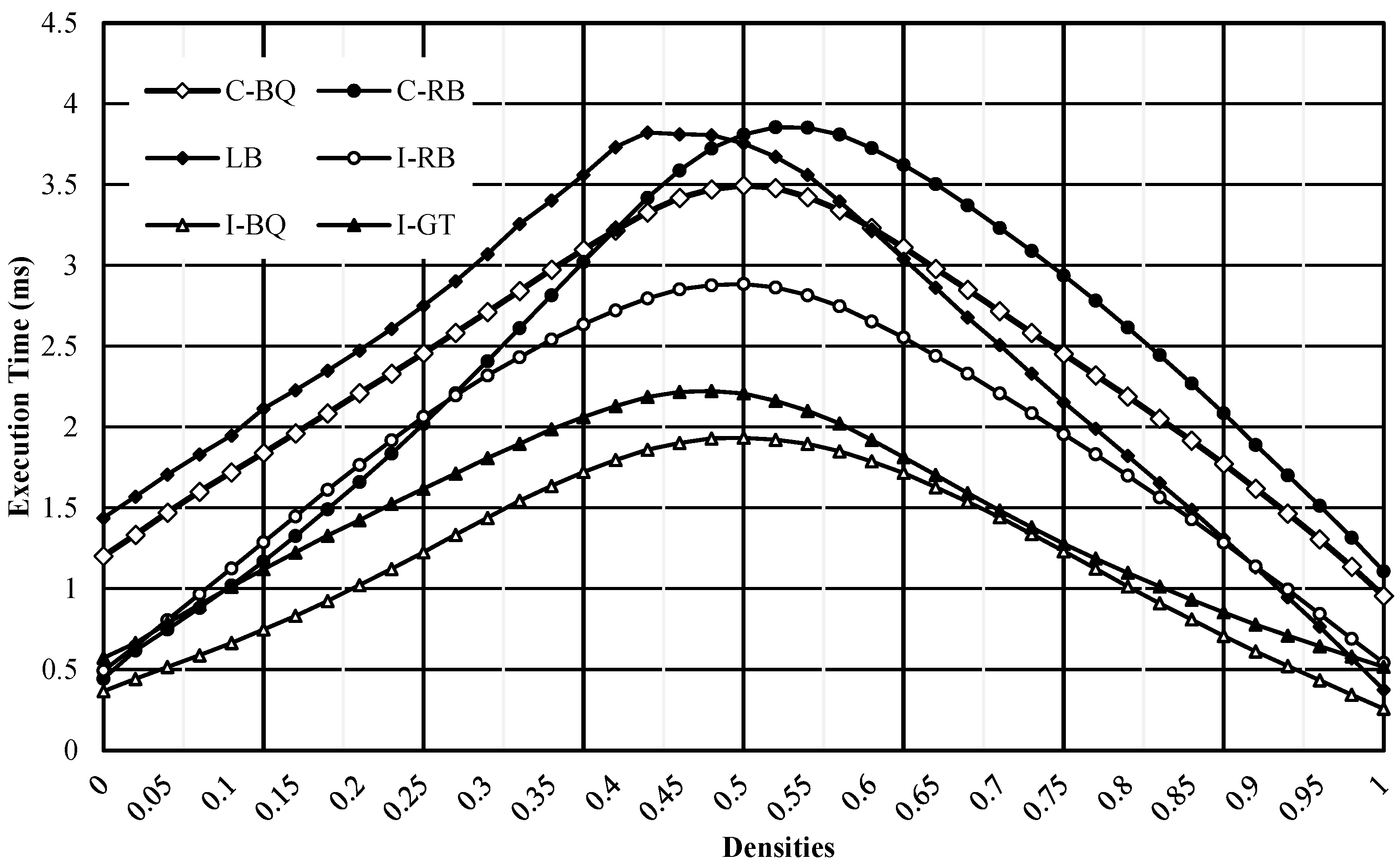
3.1.1. Execution Time versus Density of Noise Images

In this experiment, we evaluated the execution time versus the density of the foreground pixels. This experiment was performed using a set of 41 noise images, each with a resolution of 512 × 512 pixels. Figure 20 and Table 4 exhibit the experimental findings. In Figure 20, it can be seen that for all tested images, the I-BQ algorithm was the most efficient algorithm among the compared algorithms and the I-GT algorithm outperformed all other algorithms except the I-BQ algorithm for almost all images. Meanwhile, the C-RB algorithm and the I-RB algorithm had good performance on the images with relatively low densities, and the I-RB algorithm and the LB algorithm had good performance on the images with relatively high densities.

3.1.2. Execution Time versus Resolution of Images

Due to the high degree of similarity between noise images of different resolutions, all of the generated noise images were utilized to test the linearity of algorithmic execution time in relation to image resolution. Figure 21a and Figure 21b display the maximum and average execution times, respectively, for noise images of varying resolutions. Observing Figure 21, it becomes apparent that all of the algorithms possessed highly desirable linear characteristics in terms of both maximum and average execution times across different image resolutions. Additionally, the I-BQ algorithm demonstrated significantly shorter processing times than any other algorithm when examining either the maximum or the average execution time.

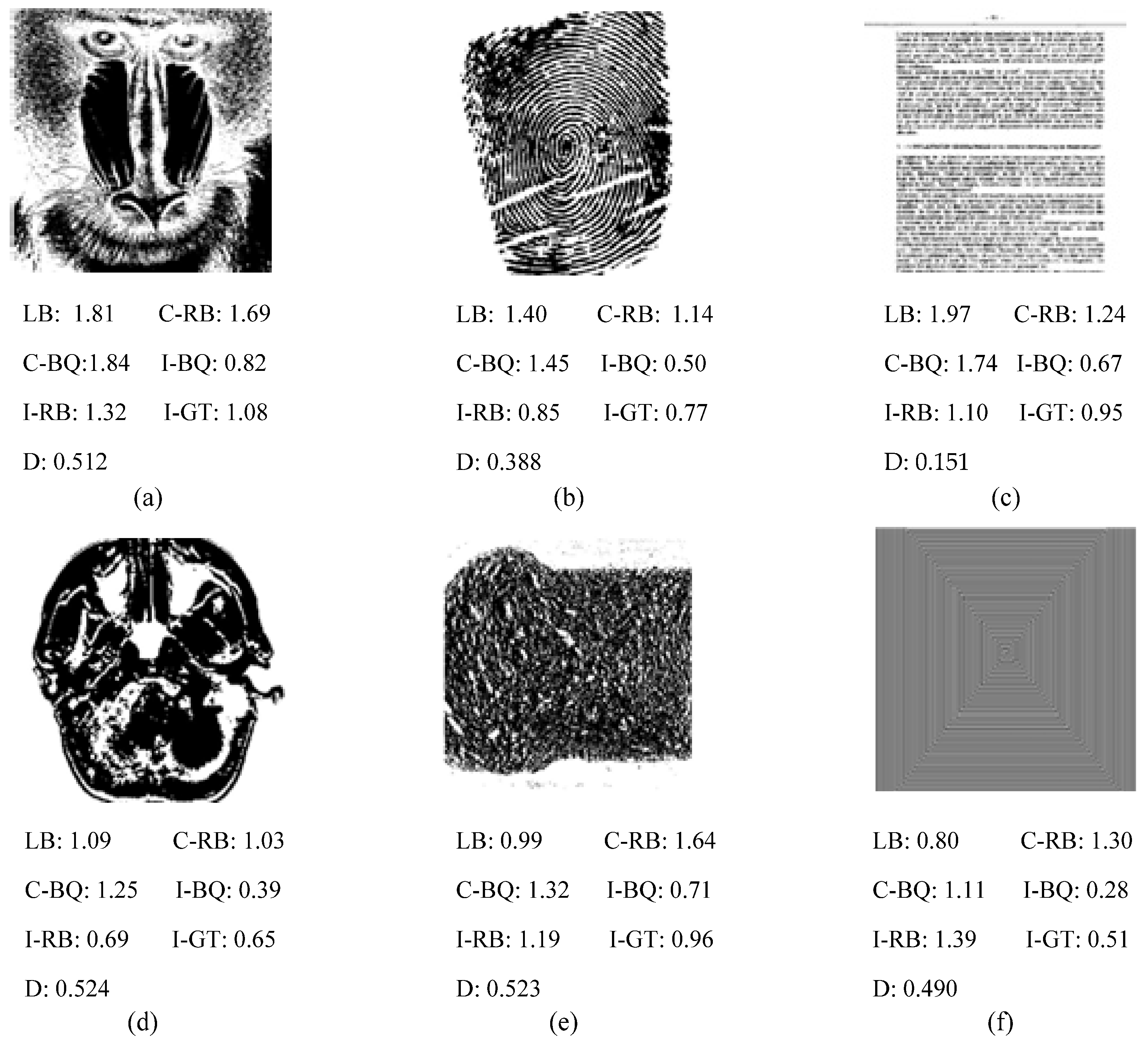
3.2. Experimental Results of Authentic Images

The authentic image dataset used in this experiment encompasses a set of 50 natural images that include text, portrait, fingerprint, aerial, snapshot, still-life, and landscape images. These images were sourced from two distinct databases: the image database of the University of Southern California and the Standard Image Database presented by the University of Tokyo. Furthermore, this experiment also utilized seven texture images downloaded from the Columbia Utrecht Reflectance and Texture Database, as well as 25 medical images obtained from a medical image database owned by the University of Chicago. Each of these images has a resolution of 512 × 512 pixels and was binarized using Otsu’s approach [43]. In addition, the experiments also included four synthetic images with distinct shapes (sawtooth-like, checkerboard-like, spiral-like, and stair-like patterns).
Table 5 displays the minimum, average, and maximum execution times of each algorithm for different kinds of images. From Table 5, it can be seen that the I-BQ algorithm was the most efficient on various kinds of images. Moreover, the performance of the I-RB algorithm and the I-GT algorithm was similar and they were more efficient than all other algorithms except the I-BQ algorithm.
Figure 22 depicts the execution time (in milliseconds) for the six chosen images, with black representing the foreground pixels and D reflecting the image’s density.

4. Relevant Issues

This section covers topics related to the parallel implementation, hardware implementation, and extension of Euler number computation algorithms for 3D images.

4.1. Parallel Implementation of Euler Number Computing Algorithms

As proven in [17], the Euler number exhibits a local additive property that permits the image to be partitioned into smaller sub-images, and the overall Euler number can then be computed by combining the individual Euler numbers of each sub-image.
Refs. [37,38] presented algorithms for calculating the Euler number based on the divide-and-conquer approach. In these algorithms, a given image is partitioned into several sub-images by cut lines in advance. Suppose I is the given image, and let L represent a cut line that divides I into two sub-images, i.e., I1 and I2. Suppose that p is a run (defined in Section 2.3.2) on cut line L and there are r runs on cut line L. We define k1(p) as the number of runs on the boundary of sub-image I1, which are neighbors of p, and k2(p) as the number of such runs in sub-image I2. Subsequently, we can compute the Euler number by using Formula (14).
E(I) = E(I1) + E(I2) + Cont(L)
Here, C o n t ( L ) = p = 1 r 1 k 1 ( p ) k 2 ( p ) .
As shown in Figure 23, image I is partitioned into I1 and I2 by cut line L. Obviously, there is one connected component and no hole in the sub-images I1 and I2; thus, the Euler number of sub-image I1 and sub-image I2 is 1.
Moreover, both k1(p) and k2(p) are 3, and C o n t ( L ) = p = 1 r 1 k 1 ( p ) k 2 ( p ) = 3 3 3 = 3 . Thus, Euler number I is E(I) = E(I1) + E(I2) + Cont(L) = 1 + 1 − 3 = −1. In fact, one connected component and two holes exist in image I, so based on the definition, the Euler number of I is 1 − 2 = −1.
Furthermore, a simple VLSI architecture is established by using some simple processors, and each processor is responsible for the Euler number computation of a sub-image. Lastly, the algorithm combines the results of the sub-images and presents the Euler number of the image. Obviously, the more sub-images are being partitioned, the more efficient the algorithm will be, theoretically. On the other hand, the more processors are being used, the more expensive the hardware devices will be.
Considering the specific instance of the image partitioning method presented in Ref. [37], if we partition an N × N-sized image I into N sub-images I1, I2, …, and IN, each row (or column) of the image will be a sub-image. According to Formula (14), we need to obtain the Euler number of each row (considered a sub-image) in the given image. At the same time, we need to count the 8-connectivity runs between two adjacent rows. As we know, holes cannot be formed in a row, and the Euler number of each row will be the number of runs in that row. Thus, we can compute the Euler number as the difference between the number of runs and that of the 8-connectivity runs, which is the run-based algorithm mentioned in Section 2.3.2.
Following the above consideration, a pipeline architecture is reported in Ref. [23] to obtain the Euler number of an image. In the reported architecture, two types of processing units, P1 and P2, are designed to calculate the Euler number. P1 is utilized to locate the beginning of a run in each row, whereas P2 indicates the start of an 8-connectivity run. To implement P1, at the start of processing each row, a delay flip-flop is set to 0, and all pixels in the row are sequentially streamed into P1. At every moment in time, the ith pixel and the (i − 1)th pixel in a row are examined for a 0→1 transition. Once a 0→1 transition is examined between the ith pixel and the (i − 1)th pixel in a row, a new run is found. On the other hand, P2 examines whether a run in a row has started or not and whether it neighbors another run in the adjacent row. The pixel values for the columns of two adjacent rows are fed sequentially to P2 through a pipeline, along with input from the delay flip-flops of those two rows. At each moment, P2 examines the ith pixel and the (i − 1)th pixel of the two adjacent rows in order to check whether there is an 8-connectivity run.
In Ref. [39], Chiavetta discussed how to use the connectivity graph derived from the cylindrical algebraic decomposition of the Euclidean plane to compute the Euler number of an image. By partitioning the given image into slices (cylinders) and constructing a connectivity graph, the algorithm finds the start of a new connected component and the end of a hole and computes the difference between them as the Euler number. Because the procedure of finding the start of a new connected component or the end of a hole can be done in the sub-images simultaneously, a parallel algorithm is proposed by using the connectivity graph.
Furthermore, the parallel architectures for obtaining the Euler number are applied to various fields of image processing, such as database search, image binarization, and image registration [40,41,42].
However, the execution speed of n parallel processes may be n times faster than that of a single processor, theoretically. Parallel implementation of an algorithm cannot guarantee acceleration in the case of simple computation because various parts of the work need to be allocated to different processing processes or threads, and parallel processing cannot be automatically implemented due to interrelated issues. For complex computational work, the efficiency of parallel implementation is generally higher than non-parallel implementation.

4.2. Euler Number Computation of 3D Images

A 3D image can be considered a 3D array composed of voxels (pixels in 2D images). As in 2D cases, there is different connectivity between voxels in 3D images. For voxels M = (m1, m2, m3) and N = (n1, n2, n3), M and N are 6-connectivity when |m1n1| + |m2n2| + |m3n3| = 1, whereas M and N are 26-connectivity when max (|m1n1|, |m2n2|, |m3n3|) = 1. For example, as presented in Figure 24, p1, p3, p5, p7, p17, and p26 are 6-connectivity voxels to voxel p and voxels p1, p2, …, and p26 are 26-connectivety voxels to voxel p [44].
Formula (15) defines the Euler number for a 3D image, which is commonly utilized to describe intricate microstructures [45,46].
E = OH + C
Here, the total number of connected components in the image is denoted by O, whereas H represents the total number of holes (or tunnels) and C represents the total number of cavities (or bubbles) present in the 3D image [47,48]. According to the definition, Akira and Aizawa [44] proposed a one-pass algorithm that utilizes an n × n array of finite-state automata to calculate the number of connected components, cavities, and holes in a 3D image. Then, the Euler number can be calculated using Formula (15). In order to calculate the Euler number based on Formula (15), as with 2D images, the number of connected components, cavities, and holes in the 3D image needs to be obtained. In this case, the classical labeling algorithm needs to be used to label them.
In order to avoid the complex labeling process, many algorithms have been presented that use alternative methods to calculate the Euler number of a 3D image. Some algorithms are derived from those in 2D image cases, such as the perimeter-based algorithm [12], the run-based algorithm [49,50], and the corner codification-based algorithm [51]. Furthermore, some algorithms are reported only for 3D images. For example, one proposed algorithm, presented by Lee and Poston [52], involves smoothing a 3D image to a differentiable object and applying theorems from differential geometry and algebraic topology. Another alternative method was presented by Sánchez-Cruz et al. [53], which calculates the Euler number of a voxelized object with tunnels and/or cavities by analyzing the relationship between contact voxel faces and enclosing surfaces. Moreover, a formula based on surface calculations was proposed by Čomića [54] for computing the Euler number of an arbitrary object in a cubical grid that has either vertex- or face-adjacency. This method involves counting only the boundary faces and vertices of the object while also adjusting the vertex count to account for the two adjacency relations.
Park and Rosenfeld [47] provided a voxel pattern-based method for calculating the 6-adjacent Euler number in a 3D image via the statistics of specific 2 × 2 × 2 voxel patterns. For a case in which 26-adjacency is considered, Morgenthaler solved the problem in Ref. [55]. To obtain the Euler number, these algorithms need to count specific 2 × 2 × 2 voxel patterns, and they are easy to implement in practice. However, some voxels are accessed repeatedly in these algorithms. Recently, Yao et al. [56] presented an improved voxel pattern-based algorithm by changing the access order and combining some voxel patterns that have the same Euler number increments. Although it is more efficient than the algorithm presented by Morgenthaler, it can be further improved by hardware implementation.

5. Concluding Remarks

The focus of this paper is to provide an overview of the latest and most advanced algorithms for computing the Euler number that have been proposed in recent decades. We aim to introduce the main strategies and techniques utilized in these algorithms. Based on experimental results from different types of images, the improved bit-quad-based I-BQ algorithm proved to be the most efficient in almost all cases. However, when the objective is to identify connected components in an image, it would be more appropriate to choose the LB algorithm. In additional, parallel implementation and hardware implementation for computing the Euler number of 2D images are discussed in this paper, and we provide an extension to Euler number computing algorithms of 3D images. Notably, both the bit-quad-based and run-based Euler number computation approaches process pixels in a raster scan order, making them well suited for parallelization. In terms of future research directions for the Euler number computing problem, the following areas warrant further consideration:
(1)
To further improve the efficiency of Euler number computing for embedded image-processing systems, it would be worthwhile to explore hardware implementation and parallel implementation of the bit-quad-based and run-based algorithms on multiple FPGAs (field programmable gate arrays).
(2)
Efficient hardware and parallel implementations of the latest Euler number computing algorithms for 3D and higher-dimensional images could be pursued to improve the processing efficiency for such complex image data.

Author Contributions

Conceptualization, B.Y. and L.H.; methodology, B.Y.; software, H.H.; validation, S.K. and H.H.; formal analysis, Y.C.; investigation, Y.C.; resources, S.K.; data curation, L.H.; writing—original draft preparation, B.Y.; writing—review and editing, L.H.; supervision, L.H.; project administration, L.H.; funding acquisition, L.H. and B.Y. All authors have read and agreed to the published version of the manuscript.

Funding

This research was funded in part by the National Natural Science Foundation of China under grant Nos. 61971272 and 61603234; the Nitto Foundation, Japan; the Hibi Science Foundation, Japan; and the Scientific Research Foundation of Shaanxi University of Science and Technology under grant No. 2020BJ-18.

Data Availability Statement

The data presented in this study are available on request from the corresponding author.

Conflicts of Interest

The authors declare no conflict of interest.

References

  1. Yang, H.; Sengupta, S. Intelligent shape recognition for complex industrial tasks. IEEE Control Syst. Mag. 1988, 8, 23–30. [Google Scholar] [CrossRef]
  2. Hashizume, A.; Suzuki, R.; Yokouchi, H.; Horiuchi, H.; Yamamoto, S. An algorithm of automated RBC classification and its evaluation. Bio Med. Eng. 1990, 28, 25–32. [Google Scholar]
  3. Nayar, S.; Bolle, R. Reflectance-based object recognition. Int. J. Comput. Vis. 1996, 17, 219–240. [Google Scholar] [CrossRef]
  4. Rosin, P.; Ellis, T. Image difference threshold strategies and shadow detection. In Proceedings of the British Machine Vision Conference, Birmingham, UK, 10–13 September 1995; pp. 347–356. [Google Scholar]
  5. Moraru, L.; Cotoi, O.; Szendrei, F. Euler number: A method for statistical analysis of ancient pottery porosity. Eur. J. Sci. Theol. 2011, 7, 99–108. [Google Scholar]
  6. Qin, X.; Xia, Y.; Wu, J.; Sun, C.; Zeng, J.; Xu, K.; Cai, J. Influence of pore morphology on permeability through digital rock modeling: New insights from the Euler number and shape factor. Energy Fuels 2022, 36, 7519–7530. [Google Scholar] [CrossRef]
  7. Gonzalez, R.; Woods, R. Digital Image Processing, 3rd ed.; Pearson Prentice Hall: Upper Saddle River, NJ, USA, 2008; pp. 642–647. [Google Scholar]
  8. Bovik, A.C. The Essential Guide to Image Processing, 2nd ed.; Academic Press: Cambridge, MA, USA; Elsevier: Amsterdam, The Netherlands, 2009; pp. 70–75. [Google Scholar]
  9. He, L.; Chao, Y. A very fast algorithm for simultaneously performing connected-component labeling and Euler number computing. IEEE Trans. Image Process. 2015, 24, 2725–2735. [Google Scholar]
  10. He, L.; Chao, Y.; Suzuki, K. An algorithm for connected-component labeling, hole labeling and Euler number computing. J. Comput. Sci. Technol. 2013, 28, 468–478. [Google Scholar] [CrossRef]
  11. Juan, L.; Sossa, J. On the computation of the Euler number of a binary object. Pattern Recognit. 1996, 29, 471–476. [Google Scholar]
  12. Bribiesca, E. Computation of the Euler number using the contact perimeter. Comput. Math. Appl. 2010, 60, 1364–1373. [Google Scholar] [CrossRef]
  13. Bribiesca, E. Measuring 2D shape compactness using the contact perimeter. Comput. Math. Appl. 1997, 33, 1–9. [Google Scholar] [CrossRef]
  14. Sossa, J.; Cuevas, E.; Zaldivar, D. Alternative way to compute the Euler number of a binary image. J. Appl. Res. Technol. 2011, 9, 335–341. [Google Scholar]
  15. Sossa, J.; Espino, E.; Santiago, R.; López, A.; Ayala, A.; Jimenez, E. Alternative formulations to compute the binary shape Euler number. IET Comput. Vis. 2014, 8, 171–181. [Google Scholar]
  16. Sossa, J.; Santiago, R.; Pérez, M.; Espino, E. Computing the Euler number of a binary image based on a vertex codification. J. Appl. Res. Technol. 2013, 11, 360–370. [Google Scholar] [CrossRef]
  17. Gray, S.B. Local properties of binary images in two dimensions. IEEE Trans. Comput. 1971, C–20, 551–561. [Google Scholar] [CrossRef]
  18. Thompson, C.; Shure, L. Image Processing Toolbox; The Math Works Inc.: Natick, MA, USA, 2017. [Google Scholar]
  19. Yao, B.; Wu, H.; Yang, Y.; Chao, Y.; Ohta, A.; Kawanaka, H.; He, L. An efficient strategy for bit-quad-based Euler number computing algorithm. IEICE Trans. Inf. Syst. 2014, E97–D, 1374–1378. [Google Scholar] [CrossRef]
  20. Yao, B.; He, L.; Kang, S.; Zhao, X.; Chao, Y. Bit-quad-based Euler number computing. IEICE Trans. Inf. Syst. 2017, E100–D, 2197–2204. [Google Scholar] [CrossRef]
  21. Gomez, W.; Sossa, J.; Arce, F. Finding the optimal bit-quad patterns for computing the Euler number of 2D binary image using simulated annealing. In Proceedings of the 13th Mexican Conference on Pattern Recognition, Mexico City, Mexico, 23–26 June 2021; pp. 240–250. [Google Scholar]
  22. Sossa, J.; Carreón, Á.; Santiago, R.; Bribiesca, E.; Petrilli-Barceló, A. Efficient computation of the Euler number of a 2-D binary image. In Proceedings of the 15th Mexican International Conference on Artificial Intelligence, Cancún, Mexico, 23–28 October 2016; pp. 401–413. [Google Scholar]
  23. Bishnu, A.; Bhattacharya, B.; Kundu, M.; Murthy, C.; Acharya, T. A pipeline architecture for computing the Euler number of a binary image. J. Syst. Archit. 2005, 51, 470–487. [Google Scholar] [CrossRef]
  24. Lin, X.; Sha, Y.; Ji, J.; Wang, Y. A proof of image Euler number formula. Sci. China Ser. F Inf. Sci. 2006, 49, 364–371. [Google Scholar] [CrossRef]
  25. Yao, B.; He, L.; Kang, S.; Zhao, X.; Chao, Y. A new run-based algorithm for Euler number computing. Pattern Anal. Appl. 2017, 20, 49–58. [Google Scholar] [CrossRef]
  26. Chen, M.; Yan, P. A fast algorithm to calculate the Euler number for binary images. Pattern Recognit. Lett. 1988, 8, 295–297. [Google Scholar] [CrossRef]
  27. Yao, B.; He, L.; Kang, S.; Chao, Y.; Zhao, X. A novel bit-quad-based Euler number computing algorithm. Springerplus 2015, 4, 1–16. [Google Scholar] [CrossRef] [PubMed]
  28. He, L.; Yao, B.; Zhao, X.; Yang, Y.; Shi, Z.; Kasuya, H.; Chao, Y. A fast algorithm for integrating connected-component labeling and Euler number computation. J. Real-Time Image Process. 2018, 15, 709–723. [Google Scholar] [CrossRef]
  29. Bieri, H.; Nef, W. Algorithms for the Euler Characteristic and related additive functionals of digital objects. Comput. Vis. Graph. Image Process. 1984, 28, 166–175. [Google Scholar] [CrossRef]
  30. Bieri, H. Computing the Euler characteristic and related additive functionals of digital objects from their bintree representation. Comput. Vis. Graph. Image Process. 1987, 28, 115–126. [Google Scholar] [CrossRef]
  31. Dyer, C. Computing the Euler number of an image from its quadtree. Comput. Graph. Image Process. 1981, 13, 270–276. [Google Scholar] [CrossRef]
  32. Samet, H.; Tamminen, M. Computing geometric properties of images represented by linear quadtrees. IEEE Trans. Pattern Anal. Mach. Intell. 1985, 7, 229–240. [Google Scholar] [CrossRef]
  33. Di Zenzo, S.; Cinque, L.; Levialdi, S. Run-based algorithms for binary image analysis and processing. IEEE Trans. Pattern Anal. Mach. Intell. 1996, 18, 83–89. [Google Scholar] [CrossRef]
  34. Sossa, J.; Carreón, Á.; Santiago, R.; Petrilli, A. Support vector machines applied to 2-D binary image Euler number computation. In Proceedings of the International Conference on Mechatronics, Electronics and Automotive Engineering, Cuernavaca, Mexico, 22–25 November 2016; pp. 3–8. [Google Scholar]
  35. Santiago, R. Training a multilayered perceptron to compute the Euler number of a 2-D binary image. In Proceedings of the Mexican Conference on Pattern Recognition, Guanajuato, Mexico, 22–25 June 2016; pp. 44–53. [Google Scholar]
  36. Sossa, J.; Carreón, Á.; Guevara, E.; Santiago, R. Computing the 2-D image Euler number by an artificial neural network. In Proceedings of the International Joint Conference on Neural Networks, Vancouver, BC, Canada, 24–29 June 2016; pp. 1609–1616. [Google Scholar]
  37. Dey, S.; Bhattacharya, B.; Kundu, M.; Acharya, T. A fast algorithm for computing the Euler number of an image and its VLSI implementation. In Proceedings of the International Conference on VLSI Design, Science City, India, 3–7 January 2000; pp. 330–335. [Google Scholar]
  38. Dey, S.; Bhattacharya, B.; Kundu, M.; Bishnu, A.; Acharya, T. A co-processor for computing Euler number of a binary image using divide and conquer strategy. Fundam. Inform. 2007, 76, 75–89. [Google Scholar]
  39. Chiavetta, F.; Di Gesù, V. Parallel computation of the Euler number via connectivity graph. Pattern Recognit. Lett. 1993, 14, 849–859. [Google Scholar] [CrossRef]
  40. Bishnu, A.; Bhattacharya, B.; Kundu, M.; Murthy, C.; Acharya, T. On-chip computation of Euler number of a binary image for efficient database search. In Proceedings of the International Conference on Image Processing, Thessaloniki, Greece, 7–10 October 2001; pp. 310–313. [Google Scholar]
  41. Abbasi, N.; Athow, J.; Amer, A. Real-time FPGA architecture of modified Stable Euler-number algorithm for image binarization. In Proceedings of the International Conference on Image Processing, Cairo, Egypt, 7–10 November 2009; pp. 3253–3256. [Google Scholar]
  42. Pradeep, K.; Veeraiah, N. VLSI implementation of Euler number computation and stereo vision concept for CORDIC based image registration. In Proceedings of the International Conference on Communication Systems and Network Technologies, Bhopal, India, 18–19 June 2021; pp. 269–272. [Google Scholar]
  43. Otsu, N. A threshold selection method from gray-level histograms. IEEE Trans. Syst. Man Cybern. 1979, 9, 62–66. [Google Scholar] [CrossRef]
  44. Akira, N.; Aizawa, K. On the recognition of properties of three-dimensional pictures. IEEE Trans. Pattern Anal. Mach. Intell. 1985, 7, 708–713. [Google Scholar]
  45. Velichko, A.; Holzapfel, C.; Siefers, A.; Schladitz, K.; Mücklich, F. Unambiguous classification of complex microstructures by their three-dimensional parameters applied to graphite in cast iron. Acta Mater. 2008, 56, 1981–1990. [Google Scholar] [CrossRef]
  46. Vogel, H.J.; Roth, K. Quantitative morphology and network representation of soil pore structure. Adv. Water Resour. 2001, 24, 233–242. [Google Scholar] [CrossRef]
  47. Park, C.; Rosenfeld, A. Connectivity and Genus in Three Dimensions; Computer Science Center, University of Maryland: College Park, MD, USA, 1971; Technical Report TR-156. [Google Scholar]
  48. Toriwaki, J.; Yonekura, T. Euler number and connectivity indexes of a three dimensional digital picture. Forma 2002, 17, 183–209. [Google Scholar]
  49. Lin, X.; Xiang, S.; Gu, Y. A new approach to compute the Euler number of 3D image. In Proceedings of the IEEE Conference on Industrial Electronics and Applications, Singapore, 3–5 June 2008; pp. 1543–1546. [Google Scholar]
  50. Lin, X.; Ji, J.; Huang, S.; Yang, J. A proof of new formula for 3D images Euler number. Pattern Recognit. Artif. Intell. 2010, 23, 52–58. [Google Scholar]
  51. Sossa, J.; Rubío, E.; Ponce, V.; Sánchez, H. Vertex codification applied to 3-D binary image Euler number computation. Adv. Soft Comput. 2019, 11835, 701–713. [Google Scholar]
  52. Lee, C.; Poston, T. Winding and Euler numbers for 2D and 3D digital images. Graph. Models Image Process. 1991, 53, 522–537. [Google Scholar] [CrossRef]
  53. Sánchez, H.; Sossa, J.; Braumann, U.-D.; Bribiesca, E. The Euler-Poincaré formula through contact surfaces of voxelized objects. J. Appl. Res. Technol. 2013, 11, 65–78. [Google Scholar] [CrossRef]
  54. Čomića, L.; Magillo, P. Surface-based computation of the Euler characteristic in the cubical grid. Graph. Models 2020, 112, 101093. [Google Scholar] [CrossRef]
  55. Morgenthaler, D. Three-Dimensional Digital Image Processing; University of Maryland: College Park, MD, USA, 1981. [Google Scholar]
  56. Yao, B.; He, H.; Kang, S.; Chao, Y.; He, L. Efficient strategies for computing Euler number of a 3d binary image. Electronics 2023, 12, 1726. [Google Scholar] [CrossRef]
Figure 1. Illustration of 4-connectivity and 8-connectivity between pixels: (a) the different connectivity pixels of pixel p; (b) different number of connected components under different connectivity.
Electronics 12 04406 g001
Figure 2. An example for explaining the Euler number of different types of connectivity of an image.
Electronics 12 04406 g002
Figure 3. Labeling mask in Ref. [10]: (a) working mask for labeling connected components; (b) working mask for labeling holes.
Electronics 12 04406 g003
Figure 4. An example for illustrating the skeleton-based Euler number computation: (a) A skeletonized image with a crossing pixel p2; (b) decomposing the result of pixel p2.
Electronics 12 04406 g004
Figure 5. Illustration of the perimeter and contact perimeter: (a) an image comprising 18 pixels; (b) perimeter of the image shown in (a); (c) contact perimeter of the image shown in (a).
Electronics 12 04406 g005
Figure 6. An example to illustrate the erosion procedure: (a) the structural element; (b) the given image; (c) the eroded result.
Electronics 12 04406 g006
Figure 7. An example illustrating the corner codification-based Euler number computing algorithm: (a) different codifications of each exterior corner of a contour pixel; (b) codification of an image; (c) codification of the deformed image.
Electronics 12 04406 g007
Figure 8. Three types of bit-quads need to be addressed in the C-BQ algorithm.
Electronics 12 04406 g008
Figure 9. Illustration of the problems in the C-BQ algorithm.
Electronics 12 04406 g009
Figure 10. Four states defined when processing a pixel with the state transition strategy.
Electronics 12 04406 g010
Figure 11. An example to illustrate the run-based Euler number computing algorithm.
Electronics 12 04406 g011
Figure 12. An example to illustrate the 4-connectivity graph-representing-based Euler number computing algorithm.
Electronics 12 04406 g012
Figure 13. An example to illustrate the 8-connectivity graph-representing-based Euler number computing algorithm.
Electronics 12 04406 g013
Figure 14. Illustration of processing a bit-quad to calculate edges.
Electronics 12 04406 g014
Figure 15. An example illustrating a binary tree-representing procedure of an image: (a) the given image; (b) the dividing result of the given image; (c) the binary tree corresponds to the given image.
Electronics 12 04406 g015
Figure 16. An example illustrating the algorithm proposed in Ref. [31]: (a) the given image; (b) the quadtree corresponds to the given image; (c) the dividing result of the given image.
Electronics 12 04406 g016
Figure 17. An example illustrating the graph run-representing-based Euler number computing algorithm: (a) the given image; (b) the graph corresponds to the given image.
Electronics 12 04406 g017
Figure 18. Structure of the SVM Euler number computing method.
Electronics 12 04406 g018
Figure 19. Noise images with various densities.
Electronics 12 04406 g019
Figure 20. Experimental results of execution time versus image density.
Electronics 12 04406 g020
Figure 21. Execution time versus image sizes: (a) the maximum execution time; (b) the average execution time.
Electronics 12 04406 g021aElectronics 12 04406 g021b
Figure 22. Execution time for the chosen images: (a) a portrait image; (b) a fingerprint image; (c) a text image; (d) a medical image; (e) a texture image; (f) an artificial image.
Electronics 12 04406 g022
Figure 23. An example illustrating the divide-and-conquer approach.
Electronics 12 04406 g023
Figure 24. Connectivity between voxels in a 3D image.
Electronics 12 04406 g024
Table 1. Configurations and Euler number increments of 16 types of bit-quads.
Pattern NamesBit-Quad PatternsΔnΔeΔfΔE = Δn − Δe + Δf
P1Electronics 12 04406 i0010000
P2Electronics 12 04406 i0021001
P3Electronics 12 04406 i0030000
P4Electronics 12 04406 i0041100
P5Electronics 12 04406 i0050000
P6Electronics 12 04406 i0061100
P7Electronics 12 04406 i007010−1
P8Electronics 12 04406 i008131−1
P9Electronics 12 04406 i0090000
P10Electronics 12 04406 i0101100
P11Electronics 12 04406 i0110000
P12Electronics 12 04406 i0121210
P13Electronics 12 04406 i0130000
P14Electronics 12 04406 i0141210
P15Electronics 12 04406 i0150110
P16Electronics 12 04406 i0161320
Table 2. Outputs of SVM1 and SVM2, corresponding to the 16 types of bit-quads.
Pattern NamesBit-Quad PatternsVectorsΔEy1y2
P1Electronics 12 04406 i001[0 0 0 0]T0−1
P2Electronics 12 04406 i002[0 0 0 1]T111
P3Electronics 12 04406 i003[0 0 1 0]T0−1
P4Electronics 12 04406 i004[0 0 1 1]T0−1
P5Electronics 12 04406 i005[0 1 0 0]T0−1
P6Electronics 12 04406 i006[0 1 0 1]T0−1
P7Electronics 12 04406 i007[0 1 1 0]T−11−1
P8Electronics 12 04406 i008[0 1 1 1]T−11−1
P9Electronics 12 04406 i009[1 0 0 0]T0−1
P10Electronics 12 04406 i010[1 0 0 1]T0−1
P11Electronics 12 04406 i011[1 0 1 0]T0−1
P12Electronics 12 04406 i012[1 0 1 1]T0−1
P13Electronics 12 04406 i013[1 1 0 0]T0−1
P14Electronics 12 04406 i014[1 1 0 1]T0−1
P15Electronics 12 04406 i015[1 1 1 0]T0−1
P16Electronics 12 04406 i016[1 1 1 1]T0−1
Table 3. The experimental platform of the compared algorithms.
NameVersion
ProcessorIntel Core i5-3470
Frequency3.20 GHz
Memory4 GB
Operating systemUbuntu Linux 16.10
GCC compiler4.2.3
Table 4. Execution time (ms) versus density of 512 × 512 pixel noise images.
DensityC-BQC-RBLBI-RBI-BQI-GT
0.0001.2020.4441.4380.4940.3660.572
0.0251.3340.6181.5700.6440.4420.664
0.0501.4720.7481.7060.8060.5160.788
0.0751.6000.8821.8300.9660.5880.902
0.1001.7201.0201.9481.1260.6641.012
0.1251.8401.1682.1141.2880.7481.120
0.1501.9621.3262.2281.4480.8321.224
0.1752.0861.4922.3481.6120.9241.328
0.2002.2101.6602.4741.7661.0221.424
0.2252.3321.8362.6081.9181.1221.524
0.2502.4562.0202.7502.0641.2261.618
0.2752.5842.2102.9022.1961.3341.712
0.3002.7122.4083.0702.3201.4381.808
0.3252.8422.6123.2562.4321.5441.896
0.3502.9742.8163.4022.5421.6361.986
0.3753.0983.0223.5602.6361.7222.062
0.4003.2183.2223.7322.7221.7962.130
0.4253.3283.4183.8222.7961.8602.186
0.4503.4183.5883.8122.8521.9022.218
0.4753.4723.7243.8062.8781.9302.224
0.5003.4963.8103.7542.8861.9342.208
0.5253.4803.8563.6722.8641.9222.162
0.5503.4243.8523.5602.8161.8962.100
0.5753.3423.8103.3962.7481.8502.022
0.6003.2323.7263.2222.6541.7881.920
0.6253.1123.6223.0422.5541.7161.814
0.6502.9803.5042.8622.4401.6281.704
0.6752.8503.3722.6782.3301.5381.592
0.7002.7183.2322.5082.2081.4421.484
0.7252.5843.0902.3302.0861.3381.380
0.7502.4522.9382.1541.9561.2321.278
0.7752.3202.7821.9901.8321.1241.186
0.8002.1902.6161.8221.7001.0141.098
0.8252.0522.4461.6541.5660.9101.014
0.8501.9162.2701.4881.4300.8100.932
0.8751.7722.0861.3101.2860.7080.854
0.9001.6201.8901.1321.1380.6120.778
0.9251.4661.7020.9480.9960.5220.710
0.9501.3061.5140.7660.8440.4340.644
0.9751.1361.3160.5700.6900.3440.580
1.0000.9561.1080.3740.5420.2580.518
Table 5. Minimum, average, and maximum execution times (ms) of the compared algorithms on different kinds of images.
Densities C-BQC-RBLBI-RBI-BQI-GT
NaturalMin.1.100.610.870.530.310.49
Average1.421.071.400.820.500.71
Max.1.861.691.971.290.821.02
MedicalMin.1.170.750.910.620.360.54
Average1.290.921.250.680.420.62
Max.1.471.071.500.840.520.73
TexturalMin.1.001.040.510.540.280.51
Average1.381.351.100.870.480.68
Max.1.731.661.601.190.710.92
ArtificialMin.0.280.240.320.170.080.11
Average0.700.670.700.480.210.28
Max.1.111.031.350.920.320.49
Disclaimer/Publisher’s Note: The statements, opinions and data contained in all publications are solely those of the individual author(s) and contributor(s) and not of MDPI and/or the editor(s). MDPI and/or the editor(s) disclaim responsibility for any injury to people or property resulting from any ideas, methods, instructions or products referred to in the content.

