Abstract
Space-based systems providing remote sensing, communication, and navigation services are essential to the economy and national defense. Users’ demand for satellites has increased sharply in recent years, but resources such as storage, energy, and computation are limited. Therefore, an efficient resource scheduling strategy is urgently needed to satisfy users’ demands maximally and get high task execution benefits. A hierarchical scheduling method is proposed in this work, which combines improved ant colony optimization and an improved deep Q network. The proposed method considers the quality of current task execution and resource load balance. The entire resource scheduling process contains two steps, task allocation and resource scheduling in the timeline. The former mainly implements load balance by improved ant colony optimization, while the latter mainly accomplishes the high task completion rate by an improved deep Q network. Compared with several other heuristic algorithms, the proposed approach is proven to have advantages in terms of CPU runtime, task completion rate, and resource variance between satellites. In the simulation scenarios, the proposed method can achieve up to 97.3% task completion rate, with almost 50% of the CPU runtime required by HAW and HADRT. Furthermore, this method has successfully implemented load balance.
1. Introduction
Satellites play an indispensable role in the national economy and defense security. They provide essential strategic support for meteorological forecasting [], disaster monitoring [], urban planning [], military investigation [], etc. The control system is the cornerstone of the satellite, ensuring that the satellite functions seamlessly to provide various services. The control system compasses several sub-systems including the power, communication, mission planning, data acquisition, and resource scheduling systems. The operation control system is responsible for facilitating resource allocation, continuously monitoring performance parameters, and optimizing the operational efficiency of the satellite [].
Increasing constellations and user demands bring more complexity to satellite resource scheduling. How to arrange tasks reasonably, optimize the allocation of onboard resources [], and maximize the service efficiency of satellites have become crucial and challenging issues in the satellite control system [,,]. On the one hand, the satellite is constantly in a highly dynamic environment. In the satellite resource scheduling process, it is crucial to consider spatio-temporal constraints. On the other hand, resources such as onboard storage and power are limited and significantly constrain the execution of satellite tasks. In addition, the adjustable degrees of freedom of onboard equipment have increased, making resource scheduling harder.
Resource scheduling systems require efficient scheduling algorithms. During each scheduling period, tasks have multiple time windows [] for execution. Additionally, each satellite’s constraints and resource statuses differ. This poses a significant challenge to the algorithms.
An efficient resource scheduling algorithm is required to mitigate the conflict between user demand and the services that satellites can provide. Our goal is to provide an efficient scheduling approach for satellite resource scheduling that can achieve load balance and fulfill as many tasks as possible. Here are the reasons. The multi-satellite resource scheduling problem has been proven NP-hard []. Many researchers treat it as a single-objective optimization problem and consider only task profit as the objective. However, in actual satellite scheduling, multi-objective optimization can be performed to satisfy better different users’ needs and the system’s constraints. Our work concentrates on the task completion rate and the load balance [,,] of different satellites within the constellation. In traditional earth observation problems, it is vital to accomplish the tasks as much as possible. However, ensuring the load balance of satellite resources is equally crucial. This approach enhances resource utilization and reduces the failure rate. Centralizing resources on one satellite may result in idle resources on other satellites. In an attack or system malfunction, meeting the following users’ needs will become difficult, and the impact during wartime is unpredictable. Multi-satellite load balancing can improve system robustness. Load balancing also significantly affects satellite edge computing [] and network communication []. Consequently, this work considers optimizing task completion profit and resource load balance.
Scientists have conducted extensive research on satellite resource scheduling methods. Multi-satellite resource optimization configuration problems are addressed using exact algorithms [,,,,], heuristic algorithms [,,], and artificial intelligence methods [,,]. However, several problems with these algorithms still exist. Larger problem scales and more complex constraints can lead to algorithmic inefficiency, even causing the algorithm to fail to converge. Moreover, simplifying multi-satellite task scheduling constraints alone is insufficient to solve practical engineering problems. Reinforcement learning is a powerful technique for solving scheduling problems without precise modeling. However, the high complexity of these problems can sometimes make it challenging to use reinforcement learning independently. One promising approach is to decompose the resource scheduling problem into sub-problems and solve them using a combination of reinforcement learning and other techniques. This can make the overall problem more manageable and result in better performance.
This work proposes a method that divides resource scheduling among satellites into task allocation and resource arrangement in the timeline. We ensure that each sub-problem has a fast and efficient solution by decomposing the complexity of the problem. A model that considers constraints containing satellite visible time windows, resource situation, task requirements, priority, and task importance is constructed. The task allocation for load balancing is accomplished through improved ant colony optimization (IACO), while the improved deep Q network (IDQN) algorithm is utilized for resource arranging in the timeline. This approach guarantees optimal scheduling for each task based on the available resources. Therefore, our proposed method provides a reasonable and feasible execution plan for resource scheduling that considers various constraints. It represents an excellent and effective solution for tackling the multi-objective optimization problem of achieving load balance while maximizing the task completion rate in resource scheduling problems.
The main contributions of this article are summarized as follows:
- A hierarchical resource scheduling framework is developed for multiple-satellite systems. It decomposes the problem into task allocation and resource arrangement in the timeline, improving the efficiency and effectiveness of the resource scheduling process in multi-satellite systems. We first designed a representation method of multiple satellites and task requirements. Furthermore, based on the complex constraints among satellites, tasks, and their capabilities, we constructed a scheduling model that considers optimization objectives, constraints, assumptions, and other factors.
- The IACO algorithm is developed to solve the task allocation problem, ensuring the load balance across the constellation. Unlike traditional methods that consider the satellite execution time windows, our proposed method instead considers each satellite’s ability to execute tasks. This reduces the complexity of task allocation and mitigates the challenge of modeling a single comprehensive solution using only one algorithm. Furthermore, a combination of the pheromone maximization strategy and the random search method is adopted to avoid convergence to the local optimism solution.
- The IDQN algorithm is utilized to resolve the problem of resource arrangement in the timeline, which can meet the requirements of tasks. Initially, a Markov decision process model is formulated for the resource arrangement problem, followed by designing state space, action space, and reward functions. The model integrates several constraints within the environment. A model is developed through training to obtain long-term benefits, which can then guide the resource scheduling plan.
The rest of this article is organized as follows. Section 2 reviews and analyzes the current status of solving algorithms in satellite resource scheduling. Section 3 formulates the multi-satellite resource scheduling problem and proposes a hierarchical solution framework that combines task allocation and resource arrangement. Section 4 provides a method for solving the task allocation problem by IACO algorithm and arranging resources in the timeline by IDQN algorithm. Section 5 reports on the experimental results under different conditions and scenarios and compares the proposed algorithm with other existing methods.
2. Literature Review
This section presents the literature review study of existing techniques of satellite resource scheduling problems. Resource scheduling is a crucial aspect of satellite operation control, which is crucial for improving efficiency and ensuring quality of service. Scholars have solved the problem of multi-satellite resource scheduling using varied approaches such as optimization modeling, exact algorithms, heuristic algorithms, meta-heuristic algorithms [,], and reinforcement learning algorithms [,,,].
The exact algorithm can find the best solution for small-scale problems, including branch and bound [], integer programming [], and dynamic programming []. Chu et al. [] created a mathematical model to solve the resource scheduling problem for in-orbit maritime target recognition in a dual satellite cluster consisting of autonomous low-resolution and agile high-resolution satellites. They utilized a branch and bound algorithm to solve it. It can secure over 60% of the total rewards from all designated targets within a specified area.
Heuristic algorithms are designed to construct feasible solutions based on specific rules which do not guarantee optimality. However, their computation time is shorter than other algorithms. He Y. et al. [] proposed a centralized edge computing scheduling framework for the task planning of multiple agile Earth observation satellites. The central node utilized the heuristic HADRT algorithm for resource scheduling, which has been proven to be optimal under specific conditions. In the experiments, the proposed algorithm completed more than 90% of the tasks in 17 of the 20 scenarios.
Metaheuristic algorithms are known for their global optimization performance and suitability for parallel processing. While these algorithms can provide acceptable solutions within a given time frame, specific algorithms tailored to the characteristics of the problem are required for practical applications to improve problem-solving efficiency and the quality of results. Kim H. et al. [] researched optimizing task scheduling for SAR satellite constellations. They modeled and solved the problem to minimize system response time using a genetic algorithm. The optimal scheduling algorithm reduced system response time by 77.5% to 90.8%. Meanwhile, Zhou et al. [] improved on this approach by developing an adaptive ant colony algorithm to solve multi-satellite resource scheduling problems with marginal decreasing imaging duration.
Artificial intelligence [] and machine learning [] have been widely implemented in recent years across different fields. They have been used in various fields, including computer vision [], personalized recommendation systems [], and intelligent machine control []. Reinforcement learning, in particular, has gained popularity due to its ability to achieve large-scale coverage and search of solution space, continuously learn and evolve from data, and display strong algorithm universality without requiring precise modeling, making it excellent for decision-making problems. It has been extensively utilized in gaming [,,] and robot control [] domains to solve sequential decision problems.
In the field of satellite scheduling, several scholars have explored the application of reinforcement learning. Huang Y. et al. [] proposed a graph-based minimum clique partition algorithm for preprocessing and then used the DDPG algorithm to solve the earth observation satellite task scheduling problem. Wei L. et al. [] investigated the agile satellite scheduling problem with multiple objectives, utilizing an approach incorporating deep reinforcement learning and parameter transfer. He Y. et al. [] divided the scheduling problem into a sequencing problem and a timing problem. They solved the sequencing problem using reinforcement learning, while HADRT solved the timing problem. Cui K. et al. [] build a dynamic task network model to solve the satellite communication resource allocation problem using the deep double-Q learning algorithm. Ren L. et al. [] solved the stereo imaging satellite scheduling problem using a block coding based on a reinforcement learning algorithm. Hu X. et al. [] proposed a method combining DRL and one heuristic algorithm for the satellite radio dynamic resource management problem, which can accelerate the convergence speed and reduce the computational overhead.
With the rising number of satellites in orbit and task requirements from observation target users, the challenges in solving satellite resource scheduling problems have increased. This has emerged as a critical limiting factor in the performance of solving algorithms. As the problem complexity and number of constraints increase, the search range of precise solving algorithms expands rapidly, leading to high computational complexity and exponential time consumption, resulting in a dimensional explosion. Although intelligent optimization algorithms can potentially provide feasible solutions, they cannot guarantee convergence or solve the problem efficiently within a specified timeframe. Reinforcement learning faces a similar challenge of useless exploration and slow convergence when solving large-scale satellite task planning problems. The current onboard intelligence restricts the application of multi-agent reinforcement learning []. On the other hand, heuristic algorithms cannot guarantee optimality, and the solutions’ quality may not meet requirements. In some cases, satellite resources may be wastefully utilized. Furthermore, the quality of heuristic algorithms depends mainly on the design of heuristic rules, and their general applicability is relatively weak. The complexity of scheduling resources among multiple satellites is exceedingly high, thus demanding highly advanced scheduling algorithms.
The multi-satellite resource scheduling problem has the characteristics of multi-task coordination, multi-resource selection, multi-optimization objectives, and multi-constraint conditions. The complexity of the problem increases exponentially as the size of the problem increases. While reinforcement learning has demonstrated impressive results for solving scheduling problems, its effectiveness can be limited for multi-satellite scheduling problems due to problems’ complexity and multiple objectives. Therefore, relying on this algorithm to solve the problem may not always be efficient. The time and space complexity of the algorithm will be unbearable, resulting in complicated and time-consuming solutions. Therefore, this article proposes a hierarchical resource scheduling framework to reduce problem complexity. Table 1 shows clearly the advantages and disadvantages of the above algorithm and the algorithm we intend to propose.

Table 1.
Comparative table between existing approaches and the proposed one.
3. Problem Description and Model Construction
The resource scheduling center is responsible for receiving task requests from different users. Each request contains information such as the task’s priority, storage, energy resources required, and so on. The resource scheduling center then preprocesses the tasks, gets their execution time window, and converts them into storage, energy, and other resource requirements. At the same time, the capability status of executing satellites within the constellation is evaluated and transmitted to the center. Subject to various constraints of the satellite, the goal is the load balance of the entire satellite constellation while assigning each task to the satellite for execution. Each satellite will receive an unordered task list and arrange the necessary resources based on the task’s execution time window. Finally, a resource arrangement plan in the timeline is given. Figure 1 illustrates the satellite resource scheduling process. Table 2 summarizes the necessary notations used in this paper.
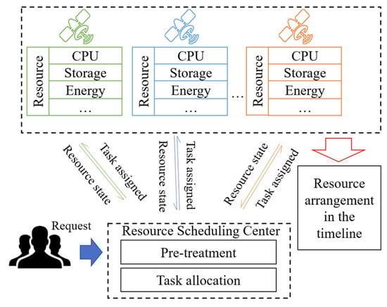
Figure 1.
Resource scheduling process of the system.
Table 2.
Summary of notations.
3.1. Assumptions
The resource scheduling process determines which satellite will provide related resources for the task. In addition, the above description is converted into a mathematical model.
Let T be the set of tasks that the users require. It can be formed as follows:
T = {task1, task2, … taskn}
taski is one of the tasks. Each task contains lots of attributes. The details are shown as follows:
taski = {ei, mi, CPUi, Profiti, [(VTWs1, VTWs1, Sat1),(VTWs2, VTWs2, Sat2),…]}
Satellites maintain relatively consistent paths in space, and the satellite’s orbit determines the feasible execution time for tasks. The multi-satellite resource scheduling problem involves allocating the relevant resources for tasks to their specific execution time and matching resources with tasks across different satellites. Due to the problem’s strong engineering background and various practical constraints, it is necessary to make reasonable assumptions and transform it into a solvable scientific problem. Thus, this paper makes the following assumptions:
- (1)
- Each task is executed once, regardless of repeated execution, which could be described as the following Equation (1);
- (2)
- After the task starts executing, it cannot be interrupted or replaced.
- (3)
- At the same time, a single satellite can only perform one task.
- (4)
- Do not consider situations where the task cannot be continued due to equipment failures.
- (5)
- The scheduled time is limited, and tasks are regularly collected and rescheduled.
3.2. Constraints
During task execution, satellites are subject to the following constraints:
- (1)
- The task must be executed within the executable time window, satisfying the corresponding Equation (3). The start time of task execution shall not be earlier than the start time of the visible time window. The end time of task execution must not be later than the end time of the visible time window;
- (2)
- The interval between the execution time of two adjacent tasks should not be less than the required switching time, which includes the startup and preheating time of different loads and the angle switching time of the same load. That is to say, the start time of the next task to execute must be later than the summary of the transition time and the end time of the task.
- (3)
- The satellite’s assigned tasks’ storage and energy requirements should not exceed its storage and energy capacity.
3.3. Objectives
Resource load balance [] should be considered an optimization goal to ensure satellites have sufficient resources to handle future tasks. Additionally, achieving the highest possible rewards during each resource scheduling cycle is essential to effectively fulfilling current users’ needs. In order to better serve current users and meet future task demands, this article proposes the following scheduling optimization objectives:
Equation (7) means one object of resource scheduling is to balance the resource load of the satellites, which is obtained by calculating the resource variance between satellites. Aveload is the average load of satellites. It is calculated as in Equation (8).
Equation (9) means the other object of task scheduling is to maximize the number of completed tasks. It is calculated by summing up the total profit of the executed tasks. Each task has a profit value in resource scheduling problems. It is obtained based on various factors like task priority and target value.
4. Hierarchical Resource Scheduling Framework
The proposed resource scheduling problem is a multi-objective, multi-constraint, and high-complexity problem. This article decomposes the resource scheduling problem into task allocation and resource arrangement to reduce problem-solving difficulty. We solve the sub-problem of task allocation by the IACO algorithm and arrange resources in the timeline by IDQN. Figure 2 shows our research methodology, which clearly illustrates the resource scheduling process.
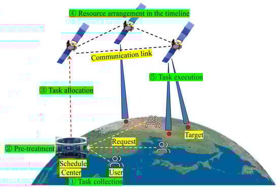
Figure 2.
A diagram of our research methodology.
Several algorithms for task allocation directly target the task time window for resource scheduling, ignoring the satellite resource situation. This may result in a small number of satellites executing most tasks. However, the hierarchical scheduling method adopted in this work comprehensively considers the load status of satellite resources and schedules resources in the timeline. During the task allocation stage, the goal is to balance the load and only consider whether the task can be executed without regard to the specific time. Resources are then scheduled during the reinforcement learning algorithm stage. Figure 3 illustrates the problem-solving process of the hierarchical resource scheduling framework. They are combined through the task assignment list. Through the IACO algorithm, each satellite can get the list of tasks to be performed, and then the IDQN is used to determine the specific execution time for tasks in the list. That is to say, the specific time for the task to get the corresponding resources is determined. The following is the detailed procedure.
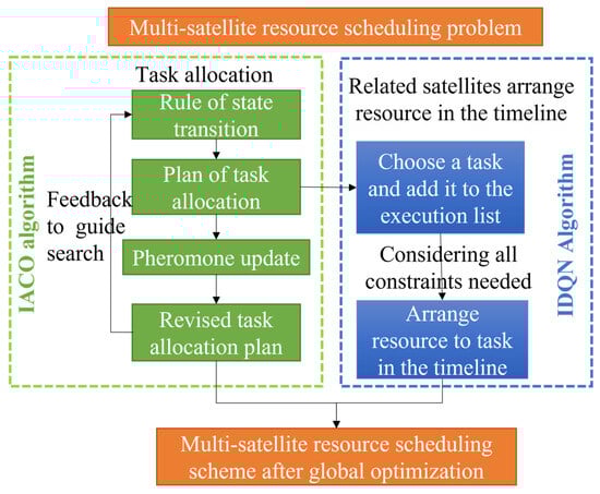
Figure 3.
Problem-solving process of hierarchical resource scheduling.
4.1. Task Allocation by IACO
The ant colony optimization algorithm was proposed by Dorigo [], inspired by exploiting the foraging behavior of ant colonies. It has demonstrated remarkable capabilities for solving complex problems such as the Traveling Salesman Problem (TSP) [] and Vehicle Routing Problem (VRP) []. The reasons why we chose IACO are as follows. The ACO algorithm is particularly suitable for solving discrete optimization problems such as resource scheduling and task allocation, and its global search capability makes it easier to find the global optimal solution. Moreover, ACO algorithms have advantages in solving large-scale and high-dimensional problems because they can parallelize processing [,]. In this article, we propose adaptive enhancements to deal with the problem of satellite task allocation. A specific fitness function is designed to evaluate the quality of task assignments. We combine random and pheromone maximization strategies to prevent the ant colony algorithm from getting stuck in local optimization. Overall, our approach builds on the strengths of the ant colony algorithm while addressing some of its limitations in solving novel optimization tasks such as satellite resource allocation.
4.1.1. The General Framework of IACO Algorithm
The pseudocode of the improved ant colony optimization process is shown in Algorithm 1:
| Algorithm 1: Improved ant colony optimization algorithm |
Optimized Objective Function: Input: original task requests and satellite resource situation Output: task allocation results Initialization: Matrixphe, Matrixtask, α, β, antNum, Iterationmax While iteration< Iterationmax do If antNum critical number Adopt the maximum pheromone strategy to allocate tasks Else Adopt the random strategy to allocate tasks Calculate the resource load variance as Equation (7) Update the pheromone matrix as Equation (13) and the task selection matrix end |
First, the resource scheduling center obtains the task executability, profit, and duration through preprocessing. Then, the parameters in IACO are initialized, such as pheromone evaporation rate α, pheromone reinforcement rate β, and task selection matrix for ants. After that, the pheromone matrix Matrixphe is initialized, expressed as follows:
where is the probability of task i being assigned to satellite j.
For each row in Matrixtask, only one value is 1, which means the task can only be executed in one satellite.
In IACO, a matrix of selection methods for tasks is defined. It can be formed as follows:
When task k was assigned to satellites, Pk means all ants before Pk choose the satellite whose pheromone is highest, while the others will select the satellite randomly.
Next, an iterative search is conducted, and the pheromone matrix is updated accordingly. If the task allocation of each generation of ants has converged or reached the maximum number of iterations, the algorithm will terminate the iteration and output the result. Otherwise, the iteration will continue.
4.1.2. The Design of the Fitness Evaluation Function
During an iteration in the ant colony algorithm, each ant will assign tasks based on selecting the maximum pheromone concentration or a random strategy. The ants then evaluate whether the assigned tasks meet the constraints for satellite energy, storage, and other factors. Allocation results that satisfy these constraints will be assessed based on the variance of the constellation load. Furthermore, the fitness evaluation function is designed. It is found according to Equation (7). It is also the objective of this subproblem. The remaining theoretical resources of each satellite are derived by subtracting the allocated resources for executing tasks provided by the IACO algorithm from their existing resources. Calculating the variance of the theoretical remaining resources across all satellites determines the load balance variance, which helps ensure efficient workload distribution.
This evaluation result will be the basis for updating the pheromone concentration at the corresponding location. For modes with minor load variances, the pheromone will increase. When the end condition is met, the algorithm will terminate the iteration and output the search results.
4.1.3. The Update of Pheromone and Search Method
The process of pheromone updating includes both pheromone evaporation and pheromone reinforcement. At the end of each iteration, all elements in the pheromone matrix are multiplied by the pheromone evaporation rate. Next, the resource load rate of the task selection scheme provided by each ant is calculated. The scheme with the minor load variance among the distribution results in that iteration is then enhanced by the corresponding location pheromone. It is updated as Equation (13). a is the task selection matrix whose load variance is minimum.
The search method update is aimed at updating the selection matrix MatrixMethod. For each element Pi in the matrix, it could be shown as in Equation (14):
where maxPheromone is the biggest pheromone value in line i of the pheromone matrix and sumPheromone is the sum of line i of the matrix. The MatrixMethod will be updated accordingly whenever the pheromone matrix is updated.
4.2. Resource Arrangement in the Timeline by IDQN
With the advancement of deep reinforcement learning, significant progress has been made in various fields. The problem is modeled as a finite Markov Decision Process (MDP) in reinforcement learning. The MDP is the theoretical framework for achieving goals through interactive learning. The agent is the part that performs the learning and implements the decisions [,]. Multi-agent system consists of multiple agents with different capabilities. Agents can operate collaboratively with each other through interaction to accomplish complex tasks. Multi-agent systems have better robustness and higher efficiency [,]. By continually interacting with the environment and receiving positive or negative feedback, agents can learn strategies that obtain long-term benefits in complex environments, leading to better decision making. The DQN algorithm breaks the limitation that Q-learning can only represent a limited state space. It adopts the experience replay mechanism, which improves the utilization of the training experience and attenuates the effect brought by the correlation of data sequences. It adopts a single-step updating method with high exploration efficiency [,]. Hence, it can be a valuable technique for optimizing the comprehensive utilization of satellite resources.
4.2.1. The MDP Modeling Process
After employing the IACO algorithm to allocate tasks, each satellite will receive a task list that balances resource utilization. However, the time for assigning the resources to perform each task has not been determined. An improved deep Q network (IDQN) algorithm is adopted to decide when the resource is allocated. Moreover, a Markov decision process is proposed to ensure the algorithm can be used. As shown in Figure 4, the agent perceives the tasks’ characteristics like profit, latitude, longitude, and resource. Then, it will select a task and add it to the queue to allocate resources. The environment will arrange resources in the timeline based on the existing queue. After that, the reward and next state will be feedback. After judging whether the next state is the terminate state, we will turn to the next training episode or update the value function. After reaching the maximum training episode, the algorithm will output the best model. The best model could be used to make the best decision.
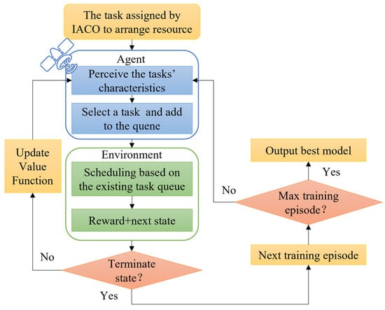
Figure 4.
The process of model training for the IDQN algorithm.
This phase guarantees timeliness between tasks and completes as many tasks as possible. In this way, the users’ demands can be satisfied as much as possible.
The algorithm accomplishes resource arrangement in the timeline by taking into account three key factors:
- (1)
- State. The state includes information about task requests and satellite status. Task information comprises visible task windows, profits, geographical coordinates, whether the task is executed, and other relative information. The status of each satellite is determined by its resource utilization level in various aspects. In the Markov decision process, the state can be expressed by the geographical coordinates, task profit, whether the task is executed, and the time window left in which the task can be executed. Other factors are integrated into the scheduling environment. The state can be expressed as S = {lani, loni, profiti, xi, windowleft}.
- (2)
- Action. In this model, the action is to choose a task not selected before or turn to the next orbiting cycle. As we all know, the satellite moves periodically along its orbit. We define that one period as an orbiting cycle. There may be more than one visible time window for a task. However, in one orbiting cycle, only one visible time window exists. If the satellite can perceive that it is better to arrange the task to the next orbiting cycle, it will not choose it this time. After all tasks that are better to execute in this orbiting cycle are selected, the satellite will turn to the next orbiting cycle.
- (3)
- Reward. The profit is obtained through interacting with the environment. It is the increment of the total profit after performing the chosen action. Furthermore, the total profit can be calculated by arranging the tasks according to the start time of the visible window under some assumptions. To enhance the task scheduling process, we begin with sorting the time window of tasks by their respective end time. Subsequently, the task with the earliest end time and evaluate the total profit generated from its implementation. The reward can be expressed as R = F(A + a) − F(A). A refers to the collection of previously executed actions. F(A) refers to the total profit from performing action set A.
4.2.2. The IDQN Training Process
As shown in Figure 5, the training process involves several steps. First, the experience pool, target network parameters, and current network parameters are initialized. Next, the agent interacts with the environment, inputting its current state into the current value network and selecting actions based on the -greedy rule. When selecting actions, they are chosen randomly with a certain probability, making it easier for the algorithm to find the global optimal solution. The action then acts on the environment, generating new states and providing profits obtained from this action. Each experience consisting of the current state (s), next state (s′), action taken (a), and the reward (r) is stored in the experience pool.
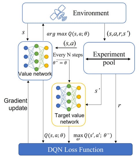
Figure 5.
The architecture of the improved deep Q-network.
After a certain number of experiences are stored, the agent begins learning. In this process, a batch of data is extracted from the experience pool and used to calculate the Q(St, At) value of the current and target networks using the TD error formula. The loss function is then calculated, back-propagation is performed, and the gradient of the current value network is updated accordingly.
The Q(St, At)value update formula can be expressed as follows:
Here, α represents the learning rate, which controls how quickly the network adapts to new experiences, while γ represents the discount factor, which determines the weight of future rewards. St+1 refers to the state in the next time step. St refers to the state of the current time step. The agent gradually learns to maximize its rewards over time by iteratively updating its networks based on these formulas.
The parameters of the target value network will be updated every N steps from the current value network. The intelligent agent in the resource scheduling system uses experience playback mechanisms, gradient updates, and other methods to continuously reduce the gap between the target network and the best value network, thereby improving the intelligence level of the resource scheduling system. By extracting data from the experience pool, the utilization rate of experience is improved. With the continuous accumulation of experience, the resources can be allocated more appropriately to tasks within the environment.
With a large number of interactions with the environment, model training gradually matures. The trained model is used for testing. At this time, there is no longer a random exploration process. The agent selects an action according to the model parameters and outputs the scheduling scheme.
4.3. Complexity Analysis
This section discusses the space complexity and time complexity of the method.
4.3.1. Space Complexity
The algorithm composition has two components, IACO and IDQN. The IDQN algorithm’s space complexity mainly comes from the experience replay pool and the neural network model.
The experience playback pool stores the current state s, action a, reward r, and the next state s’. The model is trained by calling the data in the experience pool. We take each of the four elements as a piece of experience. There are M pieces of experiences in the experience pool.
Its space complexity is CSpace(1) = M × (|s| + |r| + |a| + |s’|) = O(N).
Furthermore, the neural network model is another source of space complexity composition. In IDQN, the network input layer size is |N1|, the output layer size is |N2|, and the hidden layer size is |Nhid| for the network model size is calculated as follows,
CSpace(2) = 2 × (|N1| + |N2| + |Nhid|) = O(N).
The space complexity of the IDQN algorithm is CSpace = CSpace(1) + CSpace(2) = O(N).
The space complexity of the IACO algorithm is O(M × N).
Thus, the total space complexity is O(N) + O(M × N) = O(M × N).
4.3.2. Time Complexity
The time complexity of the IDQN algorithm is calculated as follows: the time complexity is O(N) when selecting an action. Assuming that the size of the data batch is k, if e generations are trained in the scene, the time complexity of training on the data of a scene is CTime(1) = e × k × (|s| × Nhid + Nhid × |a|) = O(N).
The time complexity of the IACO algorithm is CTime(2) = O(N4), so the total time complexity is CTime = O(N4).
Here is a table indicating the complexity of other algorithms (Table 3).
Table 3.
Complexity of algorithms.
5. Experiments and Discussion
5.1. Simulation Settings
In order to obtain the location and visibility between satellites and tasks, the multi-satellite resource scheduling problem is simulated through the software STK (Satellite Tool Kit, https://oit.ua.edu/software/stk/).
The simulation time in the experiment is set from 0:00 to 24:00 on November 9th. The tasks were generated randomly in the region between 5–55° N and 75–135° E. Figure 6 depicts the 2D and 3D graphs illustrating the distribution with 150 tasks. The task’s profit is determined based on its importance, execution time, and resource usage when the user submits it. The profit is a random number generated between 1 and 10 in simulation experiments. The duration of task execution varies across different tasks. The execution duration is set to 10 s, including a 7 s task execution time and a 3 s task switching time. There are three scenarios involving 150, 300, 450 tasks for resource scheduling.
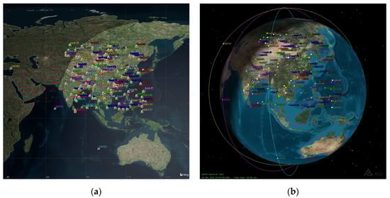
Figure 6.
Task distribution map in STK. (a) A 2D map of the task distribution; (b) A 3D map of the task distribution.
Low Earth Orbit (LEO) satellites play a significant role in various fields, including communication and remote sensing. The typical height of their orbit is below 1000 km. Three LEO satellites were selected for the simulation scenario to verify the resource scheduling algorithm. The six orbit parameters of satellites are shown in Table 4. The resource scheduling system analyzes the task after submission to obtain its resource occupation. It collects the current status of various resources at the beginning of the scheduling process. The scheduling algorithm uses the task’s resource requirements and the satellite’s resource status as input for scheduling.
Table 4.
Orbit parameters of satellites.
PyTorch is adopted as the deep reinforcement learning algorithm framework. The simulation experiments were implemented on a laptop with an Intel Core i7-127000 CPU, 16 GB Random Access Memory, Nvidia GeForce RTX 3060 GPU, and Windows 11.
Under the proposed hierarchical solution framework, load balancing among star clusters could be achieved by IACO algorithm while maximizing total profit for resource scheduling through IDQN. The pertinent parameter configurations for IACO and IDQN are presented in Table 5.
Table 5.
Parameters in IACO and IDQN algorithm.
5.2. Experimental Results
The third phase of the analysis proposes the decomposition and independent resolution of the multi-satellite resource scheduling problem, which proves to be a practical approach. Specifically, the satellite resource scheduling problem can be partitioned into two sub-problems: task allocation and resource arrangement. The IACO algorithm is employed for solving the task allocation problem, whereas an improved reinforcement learning algorithm is utilized for resource arrangement in the timeline. After task preprocessing, their executable time windows are captured. The resources utilized by the satellite, additional satellite models, and resource statuses are employed as inputs for the IACO seeking to balance storage resources and leverage other resources as scheduling constraints.
In the scenario comprising 300 tasks, the experimental outcomes depicted in Figure 7 illustrate that the task allocation results converged via the 200 iterations by IACO. Upon IACO pre-allocation, 106 tasks were assigned to satellite one. A total of 96 tasks were allocated to satellite two, and 99 tasks were allocated to satellite three, resulting in a resource load variance of 2.889. The task allocation outcomes after convergence were taken as input for the subsequent temporal scheduling level. In each task execution queue, the mandatory resources for every activity were temporally arranged using an IDQN algorithm. Figure 8 illustrates that the algorithm convergence could be achieved between 50 and 100 iterations. Nonetheless, fluctuations after convergence were due to uncertainties associated with the IDQN algorithm’s “exploration”. The model functions optimally and can provide substantial profits while demonstrating exceptional convergence capability.
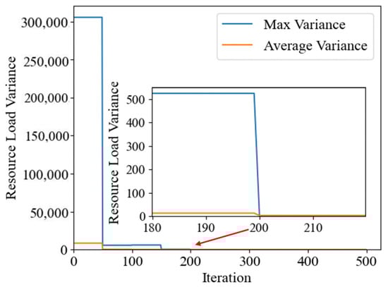
Figure 7.
Resource load variance.
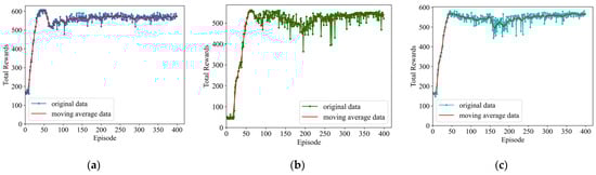
Figure 8.
Convergence of the satellite resource scheduling system. (a) The 105 task training result on SAT1; (b) The 96 task training result on SAT2; (c) The 99 task training result on SAT3.
5.3. Discussion
As far as we know, there are many advanced algorithms for satellite resource scheduling in the literature, including HADRT [], FCFS [], ALNS []. Some algorithms are applied in actual engineering, such as HAW. HADRT [] is a heuristic algorithm based on the density of remaining tasks. We design the comparison algorithm HADRT’ based on the theory of the HADRT algorithm. FCFS performs on the principle of “first come, first served” to allocate relevant resources for tasks. HAW is based on the start time of the task’s executable time window. Therefore, we choose these algorithms as comparisons. We compare and analyze the FCFS, HADRT’, and HAW algorithms with our algorithm regarding CPU runtime, resource load rate, total scheduling rewards, task completion rate, and task profit rate.
(1) The CPU runtime metric serves as a critical indicator of algorithmic efficiency. Several scheduling algorithms are simulated to evaluate real-world applicability under varying conditions. To make the results more convincing, we repeat the simulation ten times in the same condition. Our results, as shown in Table 6, indicate that the FCFS algorithm outperforms its counterparts in terms of runtime. Additionally, the combination of reinforcement learning and ant colony algorithms boasts a shorter runtime than other algorithms. Conversely, the HAW and HADRT’ algorithms exhibit the most extended runtimes, nearly twice that of the proposed algorithm. As the task size scales, CPU runtime generally increases roughly linearly.
Table 6.
CPU runtime for four algorithms.
(2) The resource load rate, as defined in Equation (7), measures the variance of resource allocation across each satellite after resource scheduling. After employing four algorithms, Table 7 depicts each scenario’s resource allocation load status. Notably, following initial task allocation using the ant colony algorithm, the variance of resource load across satellites was significantly lower than the other three algorithms. After determining the optimal scheduling timing by IDQN, the resource load rate increased, but the variance of resource allocation remained lower than that of the other three algorithms. After two resource scheduling phases, the overall resource load displayed a relatively balanced distribution among satellites. Figure 9 illustrates the variance in the final number of executed tasks per satellite for each algorithm in each scenario, with the IACO-IDQN method demonstrating the most optimal performance. We repeat the simulation 10 times in the same scenario.
Table 7.
The variance of resources.
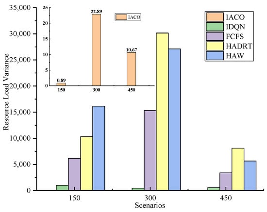
Figure 9.
The variance of resources in different satellites.
(3) In resource scheduling, the total benefit is determined by the combined benefits of the completed tasks. More tasks can be executed by scheduling resources at different times, increasing overall profit. One specific example involves scheduling resources for one satellite in scenarios where 100, 200, and 300 tasks exist. The convergence of the reinforcement learning training process is depicted in Figure 10, which shows that the algorithm converges after approximately 50 iterations, demonstrating excellent convergence properties of the adopted algorithm. This result suggests that the algorithm has obtained a relatively reliable behavioral policy after a suitable number of iterations. Furthermore, there could be an increase in both stability and total reward through training. The total reward for each scenario is presented in Table 8. Analysis shows that the HAW algorithm and HADRT’ algorithm are the most effective among these three scenarios, as they can allocate resources to all tasks and generate the highest overall reward. The ACO + RL approach also flourishes, providing approximately 93.26% of total task rewards. FCFS has the lowest total return across tasks and performs poorly as task size increases.
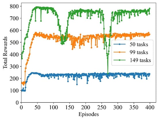
Figure 10.
Total rewards in the training process for different task numbers.
Table 8.
Total rewards in resource scheduling for four algorithms.
(4) The metrics of task profit rate and task completion rate indicate the efficiency of the resource allocation algorithms. They are calculated as Equations (16) and (17). Figure 11 shows different algorithms’ profit rate and completion rate when faced with 150, 300, and 450 tasks. Upon considering both metrics, the HADRT’ and HAW algorithms allocate required resources to tasks. In contrast, the overall task profit and task completion rate of the FCFS algorithm system is the lowest, exhibiting changes in the single-satellite indicator ranging from 30% to 90%, as well as an average task completion rate and yield of 59.74% and 60.08%, respectively. The system is greatly affected by the location of task requests. The proposed IACO-IDQN scheduling framework demonstrates the ability to provide solutions in the timeline, with task completion rates exceeding 90% in most cases, an average task completion rate of 94.74%, and an average task yield of 93.27%. The only exception lies in the case where the total number of tasks amounts to 150, wherein the task profit and completion rates of Satellite 1 and Satellite 2 are slightly below 90%.
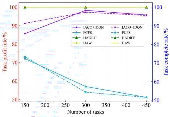
Figure 11.
The task completion rate and task profit rate for four algorithms.
As shown in Table 9, FCFS uses the shortest CPU time and can give a solution faster, but the quality is poorer among all the algorithms. The consumption time of IACO-IDQN is in the middle of the range. The reason is that the IDQN algorithm has a shorter time to apply the model in the testing process, but the IACO algorithm runtime increases as the task size increases, resulting in the consumption time of the whole framework also increasing. IACO-IDQN performs the best in the variance of satellite resources, which is much lower than other algorithms because we take load balancing as the optimization objective in this phase when IACO solves the task allocation problem. The generated solution can satisfy this condition. In the three metrics of total profit, task profit rate and task completion rate, the HADRT and HAW algorithms perform the best in the simulation scenarios to be able to complete all the tasks, while IACO-IDQN can complete 85–98% of the tasks, although not all of them. This is a result of the “exploration” factor in the IDQN algorithm, where trial-and-error learning is used for interaction with the environment, and this uncertainty affects the metrics related to task completion.
Table 9.
Summary of algorithm comparison.
The proposed IACO-IDQN algorithm for resource scheduling performs slightly worse than the HAW and HADRT’ algorithms regarding task completion rate. However, it demonstrates a decrease in scheduling time on average. Moreover, it paves the way for better performance of resource load balancing. In comparison, the FCFS algorithm is observed to possess the shortest CPU runtime, but its task completion and resource load rates are relatively poor. The distribution of tasks is found to be tremendously uneven under the FCFS algorithm, leading to many situations where the scheduled tasks remain incomplete. The HAW and HADRT’ algorithms offer the highest task profits, but their CPU runtime is comparatively longer when compared with the proposed IACO-IDQN approach. Furthermore, the CPU runtime of these algorithms increases with the growth of task size. Considering parameters like resource load, task completion rate, and algorithm running time, IACO-IDQN can yield a relatively optimized solution within a shorter duration. Moreover, it facilitates achieving resource load balancing within the constellation.
6. Conclusions
This paper investigates the resource scheduling problem for the satellite control system. It models resource and time constraints involved in multi-satellite scheduling. In order to alleviate the complexity of the problem, a hierarchical framework that decomposes it into task allocation and resource arrangement in the timeline is proposed. The goal of satellite resource load balance is achieved by IACO algorithm for task allocation, while IDQN maximizes the benefits of task execution during the resource scheduling process. The simulation results revealed that our approach can effectively deal with the dynamic environment of satellite resource scheduling problems and outperforms the FCFS, HADRT’ and HAW algorithms regarding resource load balance and algorithm response time. The task completion rate across the three experimental scenarios is up to 94.74%, with almost 50% of the CPU runtime required of the HADRT’ and the HAW algorithms. Moreover, the variance of resources between satellites is the minimum of the four methods.
In future work, we will improve the resource scheduling framework from the following two aspects: (1) to improve the generality of the algorithm to adapt to other satellite resource scheduling scenarios and (2) to simplify the algorithm framework to enable resource scheduling algorithms to run in orbit. The computing power for satellites in orbit is less than that in simulation.
Author Contributions
Conceptualization, Y.L.; methodology, Y.L.; software, Y.L. and X.M.; validation, X.L.; formal analysis, Y.L.; investigation, S.R.; resources, Y.L.; data curation, Y.L.; writing—original draft preparation, Y.L.; writing—review and editing, X.G., J.Q. and Z.M.; supervision, X.G. and J.Y.; project administration, X.G. All authors have read and agreed to the published version of the manuscript.
Funding
This research received no external funding.
Data Availability Statement
Not applicable.
Acknowledgments
The authors thank the editor, the anonymous reviewers, and all Intelligent Instrument Laboratory members for their insightful comments and feedback. The authors thank Yongming He at the National University of Defense Technology for giving them suggestions.
Conflicts of Interest
The funders had no role in the design of the study; in the collection, analyses, or interpretation of data; in the writing of the manuscript, or in the decision to publish the results.
References
- Kim, M.; Song, H.; Kim, Y. Direct Short-Term Forecast of Photovoltaic Power through a Comparative Study between COMS and Himawari-8 Meteorological Satellite Images in a Deep Neural Network. Remote Sens. 2020, 12, 2357. [Google Scholar] [CrossRef]
- Li, Z.; Xie, Y.; Hou, W.; Liu, Z.; Bai, Z.; Hong, J.; Ma, Y.; Huang, H.; Lei, X.; Sun, X.; et al. In-Orbit Test of the Polarized Scanning Atmospheric Corrector (PSAC) Onboard Chinese Environmental Protection and Disaster Monitoring Satellite Constellation HJ-2 A/B. IEEE Trans. Geosci. Remote Sens. 2022, 60, 4108217. [Google Scholar] [CrossRef]
- Barra, A.; Reyes-Carmona, C.; Herrera, G.; Galve, J.P.; Solari, L.; Mateos, R.M.; Azañón, J.M.; Béjar-Pizarro, M.; López-Vinielles, J.; Palamà, R.; et al. From satellite interferometry displacements to potential damage maps: A tool for risk reduction and urban planning. Remote Sens. Environ. 2022, 282, 113294. [Google Scholar] [CrossRef]
- Sun, F.; Zhou, J.; Xu, Z. A holistic approach to SIM platform and its application to early-warning satellite system. Adv. Space Res. 2018, 61, 189–206. [Google Scholar] [CrossRef]
- Zhang, B.; Wu, Y.; Zhao, B.; Chanussot, J.; Hong, D.; Yao, J.; Gao, L. Progress and Challenges in Intelligent Remote Sensing Satellite Systems. IEEE J.-STARS 2022, 15, 1814–1822. [Google Scholar] [CrossRef]
- Hao, Y.; Song, Z.; Zheng, Z.; Zhang, Q.; Miao, Z. Joint Communication, Computing, and Caching Resource Allocation in LEO Satellite MEC Networks. IEEE Access 2023, 11, 6708–6716. [Google Scholar] [CrossRef]
- Peng, D.; Bandi, A.; Li, Y.; Chatzinotas, S.; Ottersten, B. Hybrid Beamforming, User Scheduling, and Resource Allocation for Integrated Terrestrial-Satellite Communication. IEEE Trans. Veh. Technol. 2021, 70, 8868–8882. [Google Scholar]
- Li, Y.; Feng, X.; Wang, G.; Yan, D.; Liu, P.; Zhang, C. A Real-Coding Population-Based Incremental Learning Evolutionary Algorithm for Multi-Satellite Scheduling. Electronics 2022, 11, 1147. [Google Scholar] [CrossRef]
- Xiong, J.; Leus, R.; Yang, Z.; Abbass, H.A. Evolutionary multi-objective resource allocation and scheduling in the Chinese navigation satellite system project. Eur. J. Oper. Res. 2016, 251, 662–675. [Google Scholar] [CrossRef]
- He, L.; Li, J.; Sheng, M.; Liu, R.; Guo, K.; Zhou, D. Dynamic Scheduling of Hybrid Tasks With Time Windows in Data Relay Satellite Networks. IEEE Trans. Veh. Technol. 2019, 68, 4989–5004. [Google Scholar] [CrossRef]
- Lemaıtre, M.; Verfaillie, G.; Jouhaud, F.; Lachiver, J.-M.; Bataille, N. Selecting and scheduling observations of agile satellites. Aerosp. Sci. Technol. 2002, 6, 367–381. [Google Scholar] [CrossRef]
- He, P.; Hu, J.; Fan, X.; Wu, D.; Wang, R.; Cui, Y. Load-Balanced Collaborative Offloading for LEO Satellite Networks. IEEE Internet Things J. 2023, 1. [Google Scholar] [CrossRef]
- Deng, X.; Chang, L.; Zeng, S.; Cai, L.; Pan, J. Distance-Based Back-Pressure Routing for Load-Balancing LEO Satellite Networks. IEEE Trans. Veh. Technol. 2023, 72, 1240–1253. [Google Scholar] [CrossRef]
- Gao, Y.; Yang, H.; Wang, X.; Chen, Y.; Li, C.; Zhang, X. A Fuzzy-Logic-Based Load Balancing Scheme for a Satellite-Terrestrial Integrated Network. Electronics 2022, 11, 2752. [Google Scholar] [CrossRef]
- Kumar, P.; Kumar, R. Issues and Challenges of Load Balancing Techniques in Cloud Computing: A Survey. ACM Comput. Surv. (CSUR) 2019, 51, 120. [Google Scholar] [CrossRef]
- Gures, E.; Shayea, I.; Saad, S.A.; Ergen, M.; El-Saleh, A.A.; Ahmed, N.M.O.S.; Alnakhli, M. Load balancing in 5G heterogeneous networks based on automatic weight function. ICT Express 2023, in press. [CrossRef]
- Liu, J.; Zhang, G.; Xing, L.; Qi, W.; Chen, Y. An Exact Algorithm for Multi-Task Large-Scale Inter-Satellite Routing Problem with Time Windows and Capacity Constraints. Mathematics 2022, 10, 3969. [Google Scholar] [CrossRef]
- Liu, Y.; Jin, S.; Zhou, J.; Hu, Q. A branch-and-bound algorithm for the unit-capacity resource constrained project scheduling problem with transfer times. Comput. Oper. Res. 2023, 151, 106097. [Google Scholar] [CrossRef]
- Chen, X.; Reinelt, G.; Dai, G.; Spitz, A. A mixed integer linear programming model for multi-satellite scheduling. Eur. J. Oper. Res. 2019, 275, 694–707. [Google Scholar] [CrossRef]
- Haugen, K.K. A Stochastic Dynamic Programming model for scheduling of offshore petroleum fields with resource uncertainty. Eur. J. Oper. Res. 1996, 88, 88–100. [Google Scholar] [CrossRef]
- Chu, X.; Chen, Y.; Tan, Y. An anytime branch and bound algorithm for agile earth observation satellite onboard scheduling. Adv. Space Res. 2017, 60, 2077–2090. [Google Scholar] [CrossRef]
- Song, Y.; Xing, L.; Chen, Y. Two-stage hybrid planning method for multi-satellite joint observation planning problem considering task splitting. Comput. Ind. Eng. 2022, 174, 108795. [Google Scholar] [CrossRef]
- Niu, X.; Tang, H.; Wu, L. Satellite scheduling of large areal tasks for rapid response to natural disaster using a multi-objective genetic algorithm. Int. J. Disaster Risk Reduct. 2018, 28, 813–825. [Google Scholar] [CrossRef]
- He, Y.; Chen, Y.; Lu, J.; Chen, C.; Wu, G. Scheduling multiple agile earth observation satellites with an edge computing framework and a constructive heuristic algorithm. J. Syst. Archit. 2019, 95, 55–66. [Google Scholar] [CrossRef]
- Huang, Y.; Mu, Z.; Wu, S.; Cui, B.; Duan, Y. Revising the Observation Satellite Scheduling Problem Based on Deep Reinforcement Learning. Remote Sens. 2021, 13, 2377. [Google Scholar] [CrossRef]
- Wei, L.; Xing, L.; Wan, Q.; Song, Y.; Chen, Y. A Multi-objective Memetic Approach for Time-dependent Agile Earth Observation Satellite Scheduling Problem. Comput. Ind. Eng. 2021, 159, 107530. [Google Scholar] [CrossRef]
- He, Y.; Xing, L.; Chen, Y.; Pedrycz, W.; Wang, L.; Wu, G. A Generic Markov Decision Process Model and Reinforcement Learning Method for Scheduling Agile Earth Observation Satellites. IEEE Trans. Syst. Man Cybern. Syst. 2022, 52, 1463–1474. [Google Scholar] [CrossRef]
- Kim, H.; Chang, Y.K. Mission scheduling optimization of SAR satellite constellation for minimizing system response time. Aerosp. Sci. Technol. 2015, 40, 17–32. [Google Scholar] [CrossRef]
- Zhou, Z.; Chen, E.; Wu, F.; Chang, Z.; Xing, L. Multi-satellite scheduling problem with marginal decreasing imaging duration: An improved adaptive ant colony algorithm. Comput. Ind. Eng. 2023, 176, 108890. [Google Scholar] [CrossRef]
- Song, Y.; Wei, L.; Yang, Q.; Wu, J.; Xing, L.; Chen, Y. RL-GA: A Reinforcement Learning-based Genetic Algorithm for Electromagnetic Detection Satellite Scheduling Problem. Swarm Evol. Comput. 2023, 77, 101236. [Google Scholar] [CrossRef]
- Wen, Z.; Li, L.; Song, J.; Zhang, S.; Hu, H. Scheduling single-satellite observation and transmission tasks by using hybrid Actor-Critic reinforcement learning. Adv. Space Res. 2023, 71, 3883–3896. [Google Scholar] [CrossRef]
- Li, J.; Wu, G.; Liao, T.; Fan, M.; Mao, X.; Pedrycz, W. Task Scheduling under A Novel Framework for Data Relay Satellite Network via Deep Reinforcement Learning. IEEE Trans. Veh. Technol. 2022, 72, 6654–6668. [Google Scholar] [CrossRef]
- Ortiz-Gomez, F.G.; Lei, L.; Lagunas, E.; Martinez, R.; Tarchi, D.; Querol, J.; Salas-Natera, M.A.; Chatzinotas, S. Machine Learning for Radio Resource Management in Multibeam GEO Satellite Systems. Electronics 2022, 11, 992. [Google Scholar] [CrossRef]
- Wu, D.; Sun, B.; Shang, M. Hyperparameter Learning for Deep Learning-based Recommender Systems. IEEE Trans. Serv. Comput. 2023, 16, 2699–2712. [Google Scholar] [CrossRef]
- Bai, R.; Chen, Z.-L.; Kendall, G. Analytics and machine learning in scheduling and routing research. Int. J. Prod. Res. 2023, 61, 1–3. [Google Scholar] [CrossRef]
- Wang, X.; Chen, S.; Liu, J.; Wei, G. High Edge-Quality Light-Field Salient Object Detection Using Convolutional Neural Network. Electronics 2022, 11, 1054. [Google Scholar] [CrossRef]
- Lee, Y.-L.; Zhou, T.; Yang, K.; Du, Y.; Pan, L. Personalized recommender systems based on social relationships and historical behaviors. Appl. Math. Comput. 2023, 437, 127549. [Google Scholar] [CrossRef]
- Nguyen, D.H.; Sun, X.; Tretiak, I.; Valverde, M.A.; Kratz, J. Automatic process control of an automated fibre placement machine. Compos. Part A Appl. Sci. Manuf. 2023, 168, 107465. [Google Scholar] [CrossRef]
- Silver, D.; Huang, A.; Maddison, C.J.; Guez, A.; Sifre, L.; Driessche, G.v.d.; Schrittwieser, J.; Antonoglou, I.; Panneershelvam, V.; Lanctot, M.; et al. Mastering the game of Go with deep neural networks and tree search. Nature 2016, 529, 484–489. [Google Scholar] [CrossRef]
- Oroojlooyjadid, A.; Nazari, M.; Snyder, L.V.; Takáč, M. A Deep Q-Network for the Beer Game: Deep Reinforcement Learning for Inventory Optimization. Manuf. Serv. Oper. Manag. 2022, 24, 285–304. [Google Scholar] [CrossRef]
- Albaba, B.M.; Yildiz, Y. Driver Modeling Through Deep Reinforcement Learning and Behavioral Game Theory. IEEE Trans. Control Syst. Technol. 2022, 30, 885–892. [Google Scholar] [CrossRef]
- Pan, J.; Zhang, P.; Wang, J.; Liu, M.; Yu, J. Learning for Depth Control of a Robotic Penguin: A Data-Driven Model Predictive Control Approach. IEEE Trans. Ind. Electron. 2022, 70, 11422–11432. [Google Scholar] [CrossRef]
- Cui, K.; Song, J.; Zhang, L.; Tao, Y.; Liu, W.; Shi, D. Event-Triggered Deep Reinforcement Learning for Dynamic Task Scheduling in Multisatellite Resource Allocation. IEEE Trans. Aerosp. Electron. Syst. 2023, 59, 3766–3777. [Google Scholar] [CrossRef]
- Ren, L.; Ning, X.; Wang, Z. A competitive Markov decision process model and a recursive reinforcement-learning algorithm for fairness scheduling of agile satellites. Comput. Ind. Eng. 2022, 169, 108242. [Google Scholar] [CrossRef]
- Hu, X.; Wang, Y.; Liu, Z.; Du, X.; Wang, W.; Ghannouchi, F.M. Dynamic Power Allocation in High Throughput Satellite Communications: A Two-Stage Advanced Heuristic Learning Approach. IEEE Trans. Veh. Technol. 2023, 72, 3502–3516. [Google Scholar] [CrossRef]
- Qin, Z.; Yao, H.; Mai, T.; Wu, D.; Zhang, N.; Guo, S. Multi-Agent Reinforcement Learning Aided Computation Offloading in Aerial Computing for the Internet-of-Things. IEEE Trans. Serv. Comput. 2022, 16, 976–1986. [Google Scholar] [CrossRef]
- Lin, Z.; Ni, Z.; Kuang, L.; Jiang, C.; Huang, Z. Multi-Satellite Beam Hopping Based on Load Balancing and Interference Avoidance for NGSO Satellite Communication Systems. IEEE Trans. Commun. 2023, 71, 282–295. [Google Scholar] [CrossRef]
- Dorigo, M. Optimization, Learning and Natural Algorithms. Ph.D. Thesis, Politecnico Di Milano, Milano, Italy, 1992. [Google Scholar]
- Elloumi, W.; El Abed, H.; Abraham, A.; Alimi, A.M. A comparative study of the improvement of performance using a PSO modified by ACO applied to TSP. Appl. Soft Comput. 2014, 25, 234–241. [Google Scholar] [CrossRef]
- Jia, Y.H.; Mei, Y.; Zhang, M. A Bilevel Ant Colony Optimization Algorithm for Capacitated Electric Vehicle Routing Problem. IEEE Trans. Cybern. 2022, 52, 10855–10868. [Google Scholar] [CrossRef]
- Zhang, Z.; Zhang, N.; Feng, Z. Multi-satellite control resource scheduling based on ant colony optimization. Expert Syst. Appl. 2014, 41, 2816–2823. [Google Scholar] [CrossRef]
- Saif, M.A.N.; Karantha, A.; Niranjan, S.K.; Murshed, B.A.H. Multi Objective Resource Scheduling for Cloud Environment using Ant Colony Optimization Algorithm. J. Algebr. Stat. 2022, 13, 2798–2809. [Google Scholar]
- Sutton, R.; Barto, A. Reinforcement Learning: An Introduction; MIT Press: Cambridge, MA, USA, 1998. [Google Scholar]
- Danino, T.; Ben-Shimol, Y.; Greenberg, S. Container Allocation in Cloud Environment Using Multi-Agent Deep Reinforcement Learning. Electronics 2023, 12, 2614. [Google Scholar] [CrossRef]
- He, G.; Feng, M.; Zhang, Y.; Liu, G.; Dai, Y.; Jiang, T. Deep Reinforcement Learning Based Task-Oriented Communication in Multi-Agent Systems. IEEE Wirel. Commun. 2023, 30, 112–119. [Google Scholar] [CrossRef]
- Hao, J.; Yang, T.; Tang, H.; Bai, C.; Liu, J.; Meng, Z.; Liu, P.; Wang, Z. Exploration in Deep Reinforcement Learning: From Single-Agent to Multi-agent Domain. IEEE Trans. Neural Netw. Learn. Syst. 2023, 1–21. [Google Scholar] [CrossRef]
- Gao, J.; Kuang, Z.; Gao, J.; Zhao, L. Joint Offloading Scheduling and Resource Allocation in Vehicular Edge Computing: A Two Layer Solution. IEEE Trans. Veh. Technol. 2023, 72, 3999–4009. [Google Scholar] [CrossRef]
- Chen, G.; Shao, R.; Shen, F.; Zeng, Q. Slicing Resource Allocation Based on Dueling DQN for eMBB and URLLC Hybrid Services in Heterogeneous Integrated Networks. Sensors 2023, 23, 2518. [Google Scholar] [CrossRef]
- Nov, Y.; Weiss, G.; Zhang, H. Fluid Models of Parallel Service Systems Under FCFS. Oper. Res. 2022, 70, 1182–1218. [Google Scholar] [CrossRef]
- Liu, X.; Laporte, G.; Chen, Y.; He, R. An adaptive large neighborhood search metaheuristic for agile satellite scheduling with time-dependent transition time. Comput. Oper. Res. 2017, 86, 41–53. [Google Scholar] [CrossRef]
Disclaimer/Publisher’s Note: The statements, opinions and data contained in all publications are solely those of the individual author(s) and contributor(s) and not of MDPI and/or the editor(s). MDPI and/or the editor(s) disclaim responsibility for any injury to people or property resulting from any ideas, methods, instructions or products referred to in the content. |
© 2023 by the authors. Licensee MDPI, Basel, Switzerland. This article is an open access article distributed under the terms and conditions of the Creative Commons Attribution (CC BY) license (https://creativecommons.org/licenses/by/4.0/).