
Impact Mechanisms of Commutation Failure Caused by a Sending-End AC Fault and Its Recovery Speed on Transient Stability

1
State Key Laboratory of Alternate Electrical Power System with Renewable Energy Sources, North China Electric Power University, Beijing 102206, China
2
Central China Subsection of State Grid Corporation of China, Wuhan 430077, China
*
Author to whom correspondence should be addressed.
Electronics 2023, 12(16), 3439; https://doi.org/10.3390/electronics12163439
Submission received: 6 July 2023
/
Revised: 3 August 2023
/
Accepted: 11 August 2023
/
Published: 14 August 2023
(This article belongs to the Topic Power System Dynamics and Stability)
Abstract
:A sending-end AC fault may lead to commutation failure (CF) in a line-commutated converter high-voltage direct current (LCC-HVDC) system. In this paper, a theoretical analysis of the impact mechanisms of a CF and its recovery speed on the transient stability of a sending-end power system (TSSPS) is performed. Firstly, the models of the sending-end power system and DC power of CF are established; the ramp function is utilized to characterize the DC power recovery process. Secondly, the swing direction of the relative rotor angle caused by a sending-end AC fault is discussed, and the DC power flow method is employed to theoretically analyze the impacts of CF and its recovery speed on TSSPS. Next, the mathematic relations between parameters of the voltage-dependent current order limiter (VDCOL) and DC power recovery speed are further derived. It is concluded that the impacts of CF and its recovery speed on transient stability are related to the swing direction caused by a sending-end AC fault, the inertia of generators, and the location of the rectifier station. Finally, the theoretical analysis is validated by Kundur’s two-area system and IEEE 68-bus-based AC/DC asynchronous interconnection test power systems, respectively.
1. Introduction
Line-commutated converter high-voltage direct current (LCC-HVDC)-based transmission technology is widely utilized in long-distance bulk power transmission and regional power grid interconnection [1,2,3]. Currently, several regional power grids in China are interconnected asynchronously by LCC-HVDC-based transmission lines, with a rated DC voltage of up to ±1100 kV and transmission power of up to 12,000 MW [4,5]. On the one hand, the improvement in the voltage level and transmission capacity intensifies the threat of a single transmission line fault affecting the transient stability of the power system [6]. On the other hand, due to the complex coupling characteristics between AC and DC systems, the risk of a local isolated fault developing into systemic cascading failure increases [7].
Commutation failure (CF) caused by AC faults is unavoidable, according to the working principle of thyristors adopted by LCC-HVDC-based transmission technology [8], and has become a typical cascading failure. CF will cause overcurrent issues in the thyristors and severe DC power fluctuations in a short time [9,10]. From the power system perspective, severe DC power fluctuations caused by the CF and the following recovery process will significantly deteriorate the operation conditions of the synchronous generator in the power system [11,12], which is a key factor leading to the destruction of the transient stability of the sending-end power system (TSSPS). Therefore, improving the safe and stable operation level of the sending-end power system is of important practical significance.
Typically, the CF is caused by a receiving-end AC fault near the inverter station [13], whose mechanism has been intensely investigated. Researchers have concluded that CF is mainly caused by AC voltage disturbances such as AC voltage reduction [14], phase angle offset [15], and the harmonic caused by single-phase or three-phase faults [16]. Regarding the impact of CF caused by a receiving-end AC fault on the TSSPS, the sending-end power system is first equivalent to a two-machine and then a single-machine infinite-bus power system. The impact of CF on the TSSPS was analyzed by adopting the extended equal area criterion (EEAC) [17,18]. It was determined that CF will affect the TSSPS, and the crucial factors are the equivalent decreased value of DC transmission power and equivalent CF time. In [19], a linearized model for AC tie-line power oscillation was established, and the DC power fluctuation caused by the CF was regarded as the impulse response of the second-order linear system. Hence, the power oscillation peak value on AC tie-lines between two areas after the occurrence of the CF can be calculated quickly and subsequently employed as a power system stability assessment index. Next, the security and stability control measures for the sending-end power system were proposed in [20]. After the occurrence of CF, properly shortening the action time of the tripping generator at the sending-end power system and extending the reclosing time of the receiving-end power system will benefit the TSSPS. Furthermore, the DC power recovery process was considered in [21]. Based on the established power–angle relationship of the equivalent single-machine infinite-bus power system, it was determined that a faster DC power recovery speed will benefit the TSSPS.
However, the sending-end AC fault near the rectifier station might also cause CF during the recovery process after clearing the sending-end AC fault [22], and this mechanism is complex. Based on the quasi-steady-state analytical model of the inverter, it was concluded that the adverse activation of the current error controller (CEC) in the inverter is the inherent cause of CF [23]. In [24], time-varying immunity to this new CF phenomenon is obtained via experimental findings and theoretical explanations. Notably, the mechanisms of CF occurring under different fault levels are not the same [25]. The sudden increase in DC current is directly associated with CF resulting from nonserious faults, and controller interaction is the main factor of the CF occurring under serious faults. Furthermore, the characteristic difference between the CF caused by the sending-end and the receiving-end AC faults was analyzed in [26], and the rapid recovery of active power leading to the forward phase of the receiving-end bus voltage was determined to be the main cause of CF. After CF caused by a sending-end AC fault, the sending-end power system experiences two severe active power shocks. In this situation, the impacts of the CF caused by the sending-end AC fault and its power recovery process on the TSSPS are considerably different from those of the CF caused by a receiving-end AC fault, which is rarely discussed. Hence, the impact mechanisms of CF caused by a sending-end AC fault and its power recovery speed on the TSSPS are first revealed in this paper. Then, the mathematical relations between the parameters of the VDCOL and the DC power recovery speed are obtained. Hence, the TSSPS could be improved by modifying the VDCOL parameters correctly according to the revealed impact mechanisms.
The remainder of this paper is organized as follows. The models of the sending-end power system and DC power of CF are established in Section 2. In Section 3, the DC power flow method is employed to theoretically analyze the impacts of CF and its recovery speed on the TSSPS. Meanwhile, the mathematical relations between the parameters of the VDCOL and DC power recovery speed are derived in Section 4. Finally, the impact mechanisms are verified by Kundur’s two-area system and IEEE 68-bus-based AC/DC asynchronous interconnection test power systems in Section 5. Section 6 concludes this paper.
2. System Model
2.1. Model of a Sending-End Power System
For asynchronously interconnected power systems via LCC-HVDC-based transmission lines, the model of the sending-end power system is given in Figure 1 [18].
Next, the single-machine infinite-bus power system model is derived [27] as shown below.
where and are the mechanical power, and are the electromagnetic power, and are the inertia constant, and is the relative rotor angle between and .
2.2. DC Power Model of CF
Taking the inverter station as an example [28], its mathematical model can be represented by
where and are the DC current and DC voltage, and are the equivalent commutation reactance and ratio of the inverter transformer, and and are the inverter bus voltage and extinction angle.
When CF occurs, the primary concern is that the large-capacity active power transmission is blocked, resulting in the swing of relative rotor angles between generators, and sometimes leading to instability [17,21]. In order to mathematically analyze the impacts of the CF and its power recovery process on the TSSPS, the following assumptions are made:
- (1)
- The rectifier station of LCC-HVDC is regarded as the dynamic load on the corresponding bus [29].
- (2)
Next, the benchmark model of LCC-HVDC is built to simulate the CF and its recovery process, as shown in Figure 2. The blue solid line represents the transmitted DC power. The CF occurs and lasts for 20 ms, causing the transmitted DC power to decrease to zero. Then, it takes approximately 100 ms to recover from zero to the rated value, which is mainly affected by the inner DC controllers and the outer AC system [32,33].
Then, a DC power model of the CF is established based on the DC power variation characteristics during and after CF. Equation (6) shows the details of this process, in which the ramp function is utilized to characterize the DC power recovery process.
where and are the start and end times of the CF, is the rated DC power, is the DC power transmitted during the CF, and is the DC power recovery speed; a larger represents a faster DC power recovery speed.
In order to mathematically analyze the impact mechanisms of CF and its power recovery speed on the TSSPS, the DC power flow method is employed to establish the mathematical relationship between the relative rotor angle of the sending-end power system and the DC power transmitted on the LCC-HVDC [31,34], as follows:
where is the set of generator nodes, is the set of load nodes for which the rectifier nodes are regarded as parts of load nodes, , , , and are susceptance matrices, and and are rotor angles of generator nodes and phase angles of load nodes.
Finally, we obtain
3. Theoretical Analysis
Based on the established models in Section 2, the theoretical derivation process is divided into three parts according to the chain of fault events [22,23], as shown in Figure 3.
3.1. Sending-End AC Fault
Assuming that the electromagnetic power of decreases by and the electromagnetic power of decreases by when the sending-end AC fault occurs, we can determine that
Equation (9) shows the relative rotor angle will swing forward when , and it will swing backward when , as shown in Figure 4.
Hence, the impact mechanisms of the CF and its power recovery speed on the TSSPS are discussed for scenarios in which the relative rotor angle swings forward or backward. Furthermore, the equivalent reactance diagram of Figure 1 is presented in Figure 5.
Here, is the reactance between the inner nodes of and , is the reactance between the inner node of and the location of rectifier station, and is the reactance between the inner node of and the node of AC load.
Next, the electromagnetic power of in a short period can be derived based on Equation (8).
where .
According to the power balance, the electromagnetic power of is obtained.
Therefore, Equation (4) can be expressed as
We define that , then Equation (3) can be rewritten as
Finally, it can be deduced from Equations (10) and (13) that
3.2. During CF
CF may occur during recovery after the clearance of the sending-end AC fault [23], resulting in severe DC power fluctuations and further affecting the TSSPS. When a CF occurs at , assuming that the DC power instantaneously decreases to zero, and is denoted as the relative rotor angle of the power system, the mathematical relation between and the electromagnetic power of is derived according to the DC power flow method.
Similarly, the electromagnetic power of is
Then,
Finally,
Defining , and based on Equations (14) and (19), we find that
The solution structure of Equation (20) is composed of the special solution of Equation (20) () and the general solution of the corresponding homogeneous equation of Equation (20) (), as shown by Equation (21).
A special solution of Equation (21) and the general solution of its corresponding homogeneous equation are
Since , , we find that
According to the swing direction of the relative rotor angle caused by the sending-end AC fault, it can be concluded based on Equation (23) that
- (a)
- If the relative rotor angle swings forward:
- (i)
- If , , representing that the CF negatively affects the TSSPS.
- (ii)
- If , , representing that the CF does not affect the TSSPS.
- (iii)
- If , , representing that the CF positively affects the TSSPS.
- (b)
- If the relative rotor angle swings backward:
- (iv)
- If , , representing that the CF positively affects the TSSPS.
- (v)
- If , , representing that the CF does not affect the TSSPS.
- (vi)
- If , , representing that the CF negatively affects the TSSPS.
Furthermore, the impacts of the CF on the TSSPS with different system parameters are presented in Figure 6.
3.3. Recovery Process after CF
After CF, the DC system begins to recover to the rated operation state at . Based on the recovery model shown in Figure 2 and the DC power flow method, the mathematical relation between the relative rotor angle and the electromagnetic power of during the DC power recovery process is derived as follows.
Similarly, the electromagnetic power of is
Then,
Finally,
Based on Equations (14) and (28), we obtain
The solution structure of Equation (29) is composed of the special solution of Equation (29) () and the general solution of the corresponding homogeneous equation of Equation (30) (), as given in Equation (30).
A special solution of Equation (29) and the general solution of its corresponding homogeneous equation are
Since , , based on Equation (23), we can obtain
Substituting Equations (32) and (33) into Equation (30), we can solve
Therefore,
Next, the partial derivative of with respect to is
According to the Taylor expansion of trigonometric functions, we find that
Finally, the following conclusions can be drawn based on Equations (36)–(38):
- (a)
- If , , demonstrating that the greater is, the smaller will be.
- (b)
- If , , demonstrating that a greater does not affect the TSSPS.
- (c)
- If , , demonstrating that the greater is, the greater will be.
Therefore, the impacts of improving the DC power recovery speed on the TSSPS with different system parameters are given in Figure 7.
Based on the theoretical analysis given in Section 3, we can conclude that:
- (a)
- If the relative rotor angle swings forward:
- (i)
- If , the CF will negatively affect the TSSPS, and increasing will benefit the TSSPS.
- (ii)
- If , the CF and increasing will have no impact on the TSSPS.
- (iii)
- If , the CF will positively affect the TSSPS, and decreasing will benefit the TSSPS.
- (b)
- If the relative rotor angle swings backward:
- (i)
- If , the CF will positively affect the TSSPS, and decreasing will benefit the TSSPS.
- (ii)
- If , the CF and increasing will have no impact on the TSSPS.
- (iii)
- If , the CF will negatively affect the TSSPS, and increasing will benefit the TSSPS.
It should be noted that the analytical solutions, such as those shown in Equations (23) and (36), cannot be derived when the sending-end power system is a multi-machine power system because multivariate second-order differential equations are generally solved using numerical methods. However, the conclusions obtained in this section are still applicable. Equation (8) can be rewritten as
where is the number of total nodes and is the number of generator nodes.
Next, the sending-end power system could be equivalent to a two-machine power system, dividing generators into A and B clusters according to the CCCOI-RM [35]. Assuming that the rectifier bus is the k-th node, we can obtain that
4. Impact of DC Control on Recovery Speed
The DC recovery process after the CF is affected by DC inverter controllers. Here, the VDCOL is discussed, and its mathematical model is provided in Figure 8 [36,37]. The dynamic characteristic of the VDCOL is represented by
where is the time constant of the filter loop, and are the interpolation module’s upper and lower bounds of DC voltage, and are the interpolation module’s upper and lower bounds of DC current, and is the output order of the VDCOL.
It is assumed that the commutation and transmission losses are ignored and the VDCOL is ideal, i.e., . Then, the DC power transmitted by the rectifier station can be represented as
Next, is obtained by deriving Equation (43) with respect to time .
Finally, the partial derivatives of with respect to the main parameters of the VDCOL are stated as follows.
Equations (45) and (46) show that and , which indicates that the DC power recovery speed could be improved by increasing or decreasing . In addition, the correctness of Equations (45) and (46) are validated by the simulation results shown in Figure 9. The green, blue and red solid lines represent the transmitted DC power when or , and
5. Results and Analysis
5.1. Test Power System A
To verify the accuracy of the impact mechanisms presented in Section 3 and Section 4, the test power system based on Kundur’s two-area system was built on ADPSS [12]. The network topology is shown in Figure 10.
Based on the above theoretical analysis, the expression of in test power system A is
where and represent the inertia constants of and .
Meanwhile, represents the reactance between and the rectifier station; the repression of is
where is the total reactance between and ; and represent the transient reactance of and ; and , , , , , and represent the reactance between Bus-1 and Bus-5, Bus-5 and Bus-6, Bus-6 and Bus-7, Bus-7 and Bus-8, Bus-8 and Bus-9, and Bus-9 and Bus-2.
Equations (47) and (48) show that and . The value of could be modified by changing the relative values of and , also known as the generators’ inertia distribution, while the value of could be modified by changing the rectifier station’s location as follows, , when the rectifier station is located at Bus-6.
Next, the sending-end AC fault is set at Bus-5/Bus-9, causing the relative rotor angle to swing forward/backward, and the CF caused by the sending-end AC fault is simulated. The maximum/minimum relative rotor angle of the sending-end power system during the first swing is employed as the assessment index of the TSSPS, which is noted as /. The simulation results are shown in Figure 11 with different parameters of and , where and .
In addition, the parameter of the VDCOL is modified from 0.90 p.u. to 0.70 p.u. to increase . The simulation results are shown in Figure 12.
The simulation results shown in Figure 11 and Figure 12 reveal that the impacts of CF and its power recovery speed on the TSSPS are related to the swing direction caused by the sending-end AC fault, the inertia distribution of generators, and the location of the rectifier station, which further verify the accuracy of the impact mechanisms presented in Section 3 and Section 4. It should be noted that the conclusions in Section 3 are drawn under certain simplifications. Therefore, the boundary condition that the CF caused by the sending-end AC fault and its recovery speed have no impact on the TSSPS is not strictly , but near .
5.2. Test Power System B
To verify the applicability of the proposed approach when the sending-end power system is a multi-machine power system, the IEEE 68-bus-based test power system was built on ADPSS; the network topology is presented in Figure 13. The New England power system (sending-end) is connected to the New York power system (receiving-end) by an LCC-HVDC-based transmission line, and the rectifier station is located at Bus-21/Bus-56. In addition, , , , and with advanced rotor angles are divided into Cluster-A, and , , , , and are divided into Cluster-B. Next, we determine that , , and . The sending-end AC fault is set near the rectifier station, and the CF caused by the sending-end AC fault is simulated. Here, the fault type is a three-phase short circuit fault, and the fault duration is 0.1 s.
Scenario I: The rectifier station is located at Bus-21, and it is calculated based on Equation (40). in which , which is much smaller than . Meanwhile, the sending-end AC fault is set at Bus-21.
Scenario II: The rectifier station is located at Bus-21 and . Meanwhile, the sending-end AC fault is set at Bus-56.
In fault scenarios I and II, , based on and . As indicated by the blue, green, and red solid lines in Figure 14b and Figure 15b, increases as of the VDCOL decreases. As shown by the black and blue solid lines in Figure 14a,b, the relative rotor angle swings forward due to the sending-end AC fault, and is much bigger when the CF occurs, indicating that the CF negatively affects the TSSPS. Meanwhile, the is smaller when the power recovery speed increases, indicating that the faster power recovery speed positively affects the TSSPS. Similarly, as shown by the black and blue solid lines in Figure 15a,b, the relative rotor angle swings backward due to the sending-end AC fault. is much smaller when the CF occurs, indicating that the CF positively affects the TSSPS. As indicated by the blue, green, and red solid lines given in Figure 15a,b, is greater when the power recovery speed increases, indicating that a faster power recovery speed negatively affects the TSSPS. The simulation results verify the correctness of the impact mechanisms presented in Section 3 and Section 4.
Scenario III: The rectifier station is located at Bus-56, and based on Equation (40), it is determined that , which is much greater than . Meanwhile, the sending-end AC fault is set at Bus-21.
Scenario IV: The rectifier station is located at Bus-56, and . Meanwhile, the sending-end AC fault is set at Bus-56.
In fault scenarios III and IV, , based on and . As shown by the blue, green, and red solid lines in Figure 16b and Figure 17b, increases as of the VDCOL decreases. As indicated by the black and blue solid lines in Figure 16a,b, the relative rotor angle swings forward due to the sending-end AC fault, and is much smaller when CF occurs, indicating that the CF positively affects the TSSPS. Meanwhile, is greater when the power recovery speed increases, indicating that a faster power recovery speed negatively affects the TSSPS. Similarly, as shown by the black and blue solid lines given in Figure 17a,b, the relative rotor angle swings backward due to the sending-end AC fault, and is much bigger when the CF occurs, indicating that the CF negatively affects the TSSPS. As shown by the blue, green, and red solid lines in Figure 18a,b, is smaller when the power recovery speed increases, indicating that a faster power recovery speed positively affects the TSSPS. The simulation results verify the accuracy of the impact mechanisms presented in Section 3 and Section 4.
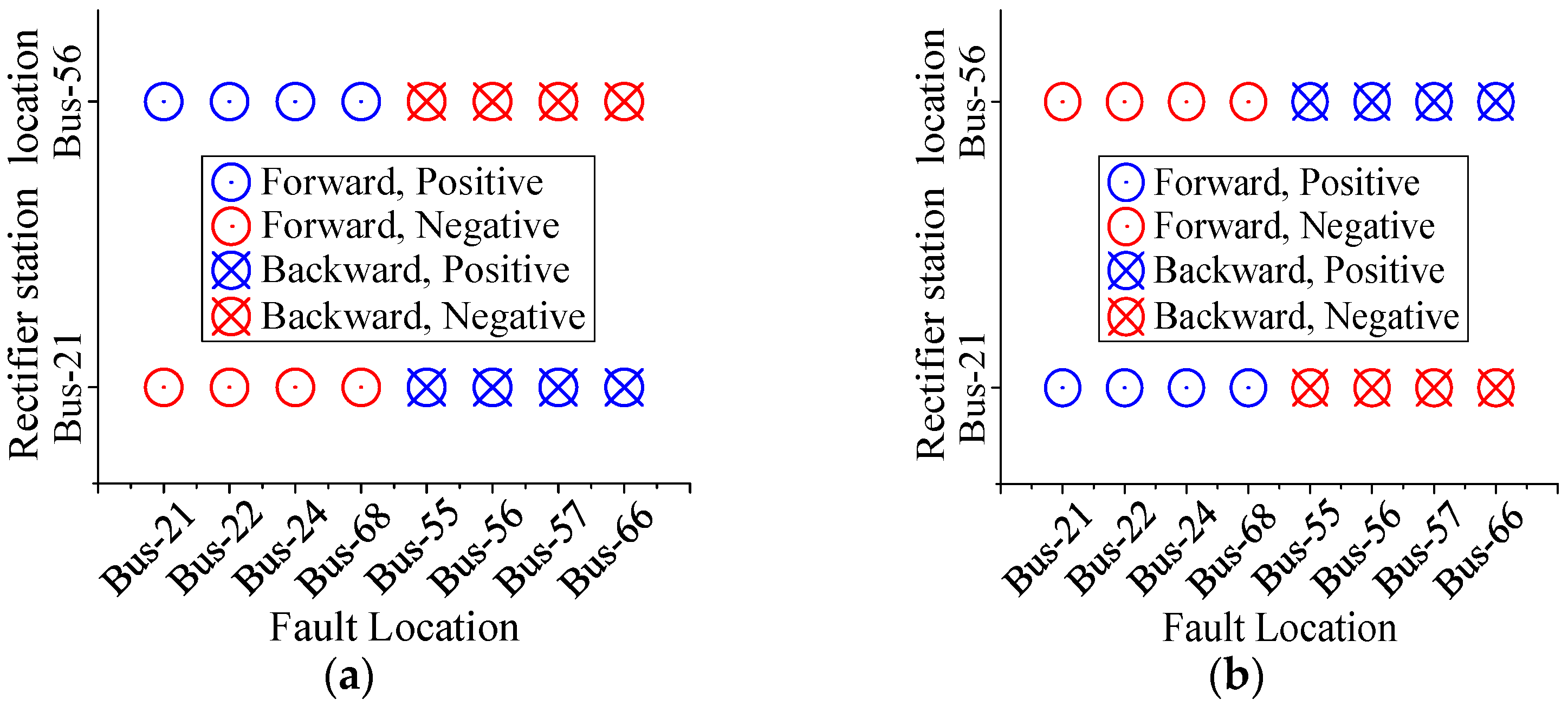
Furthermore, the sending-end AC fault is set at different buses when the rectifier station is located at Bus-21 or Bus-56. The sending-end AC fault will cause the relative rotor angle of generators to swing forward or backward. The impacts of the CF and increasing power recovery speed on the TSSPS are given in Figure 18.
In Figure 18a,b, the CF caused by the sending-end AC fault has a negative/positive impact on the TSSPS when the relative rotor angle swings forward/backward on the condition that the rectifier station is located at Bus-21. Meanwhile, the TSSPS is improved by increasing/decreasing the DC power recovery speed. On the contrary, the CF has a positive/negative impact on the TSSPS when the relative rotor angle swings forward/backward on the condition that the rectifier station is located at Bus-56. Meanwhile, the TSSPS is improved by decreasing/increasing the DC power recovery speed. The simulation results validate the accuracy of the presented impact mechanisms.
Furthermore, the impacts of the CF and its power recovery speed on the TSSPS are related to the swing direction influenced by the sending-end AC fault, the inertia distribution of generators, and the location of the rectifier station, and the TSSPS could be improved by correctly modifying the VDCOL parameters according to the presented impact mechanisms.
6. Conclusions
In this paper, the impact mechanisms of a CF caused by a sending-end AC fault and its DC power recovery speed on the TSSPS are revealed, and the mathematical relations between the parameters of the VDCOL and the DC power recovery speed are derived. The following conclusions are drawn:
- (1)
- The impacts of the CF and its DC power recovery speed on the TSSPS are related to the swing direction of the relative rotor angle, the inertia distribution of generators, and the location of the rectifier station.
- (2)
- The DC power recovery speed is positively correlated with and of the VDCOL, which indicates that the TSSPS could be improved by modifying the VDCOL parameters according to the theoretical analysis.
Regarding the concern about the TSSPS after a CF, the revealed impact mechanisms could provide a reference for improvement. For early power grid planning, the impact of a CF on the TSSPS could be reduced by reducing the difference between and . For a certain power system, as the values of and are fixed, the DC power recovery speed could be changed by modifying the parameters of the VDCOL according to its impact mechanism to improve the TSSPS.
In the future, the mathematical relations between the DC power recovery speed and the parameters of other DC controllers, as well as the electrical quantities of the receiving-end AC system, will be discussed, so that the most sensitive and cost-effective method of modifying the DC power recovery speed can be determined.
Author Contributions
Conceptualization, Z.W.; methodology, Y.L.; software, Y.L.; validation, Y.L.; formal analysis, Y.L.; investigation, J.H.; resources, Z.W.; data curation, T.W.; writing—original draft preparation, Y.L.; writing—review and editing, J.H. and T.W.; visualization, T.W.; supervision, Z.W.; project administration, Z.W.; funding acquisition, Z.W. All authors have read and agreed to the published version of the manuscript.
Funding
This work was supported by the National Nature Science Foundation of China (52277096).
Data Availability Statement
The data that support the findings of this study are available on request from the corresponding author. The data are not publicly available due to privacy or ethical restrictions.
Conflicts of Interest
The authors declare no conflict of interest.
References
- ABB. Special Report 60 Years of HVDC. 2014. Available online: https://library.e.abb.com/public/aff841e25d8986b5c1257d380045703f/140818%20ABB%20SR%2060%20years%20of%20HVDC_72dpi.pdf (accessed on 1 July 2014).
- Zhang, F.; Xin, H.; Wu, D.; Wang, Z.; Gan, D. Assessing Strength of Multi-Infeed LCC-HVDC Systems Using Generalized Short-Circuit Ratio. IEEE Trans. Power Syst. 2019, 34, 467–480. [Google Scholar] [CrossRef]
- Xiao, H.; Li, Y.; Gole, A.M.; Duan, X. Computationally efficient and accurate approach for commutation failure risk areas identification in multi-infeed LCC-HVDC systems. IEEE Trans. Power Electron. 2020, 35, 5238–5253. [Google Scholar] [CrossRef]
- Shu, Y.; Chen, G.; Yu, Z.; Zhang, J.; Wang, C.; Zheng, C. Characteristic analysis of UHVAC/DC hybrid power grids and construction of power system protection. CSEE J. Power Energy Syst. 2017, 3, 325–333. [Google Scholar] [CrossRef]
- Hu, J.; Wang, T.; Wang, Z.; Liu, J.; Bi, J. Switching System’s MLE Based Transient Stability Assessment of AC/DC Hybrid System Considering Continuous Commutation Failure. IEEE Trans. Power Syst. 2021, 36, 757–768. [Google Scholar] [CrossRef]
- Hong, L.; Zhou, X.; Liu, Y.; Xia, H.; Yin, H.; Chen, Y.; Zhou, L.; Xu, Q. Analysis and Improvement of the Multiple Controller Interaction in LCC-HVDC for Mitigating Repetitive Commutation Failure. IEEE Trans. Power Del. 2021, 36, 1982–1991. [Google Scholar] [CrossRef]
- Mirsaeidi, S.; Dong, X. An Integrated Control and Protection Scheme to Inhibit Blackouts Caused by Cascading Fault in Large-Scale Hybrid AC/DC Power Grids. IEEE Trans. Power Electron. 2019, 34, 7278–7291. [Google Scholar] [CrossRef]
- Mirsaeidi, S.; Tzelepis, D.; He, J.; Dong, X.; Mat Said, D.; Booth, C. A Controllable Thyristor-Based Commutation Failure Inhibitor for LCC-HVDC Transmission Systems. IEEE Trans. Power Electron. 2021, 36, 3781–3792. [Google Scholar] [CrossRef]
- Guo, C.; Liu, Y.; Zhao, C.; Wei, X.; Xu, W. Power Component Fault Detection Method and Improved Current Order Limiter Control for Commutation Failure Mitigation in HVDC. IEEE Trans. Power Deliv. 2015, 30, 1585–1593. [Google Scholar] [CrossRef]
- Mirsaeidi, S.; Dong, X. An Enhanced Strategy to Inhibit Commutation Failure in Line-Commutated Converters. IEEE Trans. Ind. Electron. 2020, 67, 340–349. [Google Scholar] [CrossRef]
- Xue, Y.; Zhang, X.; Yang, C. AC Filterless Flexible LCC HVDC With Reduced Voltage Rating of Controllable Capacitors. IEEE Trans. Power Syst. 2018, 33, 5507–5518. [Google Scholar] [CrossRef]
- Hu, J.; Wang, T.; Wang, Z. Transient stability margin assessment of AC/DC hybrid system with commutation failure involved. Int. J. Electr. Power Energy Syst. 2021, 131, 107056. [Google Scholar] [CrossRef]
- Thio, C.V.; Davies, J.B.; Kent, K.L. Commutation failures in HVDC transmission systems. IEEE Trans. Power Del. 1996, 11, 946–957. [Google Scholar] [CrossRef]
- Xiao, H.; Li, Y.; Zhu, J.; Duan, X. Efficient approach to quantify commutation failure immunity levels in multi-infeed HVDC systems. IET Gener. Transm. Dis. 2016, 10, 1032–1038. [Google Scholar] [CrossRef]
- Zhu, R.; Zhou, X.; Xia, H.; Hong, L.; Yin, H.; Deng, L.; Liu, Y. Commutation Failure Mitigation Method Based on Imaginary Commutation Process. J. Mod. Power Syst. Clean Energy 2022, 10, 1413–1422. [Google Scholar] [CrossRef]
- Xiao, H.; Li, Y.; Duan, X. Enhanced commutation failure predictive detection method and control strategy in multi-infeed LCC-HVDC systems considering voltage harmonics. IEEE Trans. Power Syst. 2021, 36, 81–96. [Google Scholar] [CrossRef]
- Tu, J.; Pan, Y.; Zhang, J.; Jia, J.; Qin, X.; Yi, J. Study on the stability mechanism of the sending-side three-machine-group system after multiple HVDC commutation failure. J. Eng. 2017, 2017, 1140–1145. [Google Scholar] [CrossRef]
- Tu, J.; Zhang, J.; Bu, G.; Yi, J.; Yin, Y.; Jia, J. Analysis of the sending-side system instability caused by multiple HVDC commutation failure. CSEE J. Power Energy Syst. 2015, 1, 37–44. [Google Scholar] [CrossRef]
- He, J.; Tang, Y.; Zhang, J.; Guo, Q.; Yi, J.; Bu, G. Fast Calculation of Power Oscillation Peak Value on AC Tie-Line After HVDC Commutation Failure. IEEE Trans. Power Syst. 2015, 30, 2194–2195. [Google Scholar] [CrossRef]
- Jia, J.; Zhang, J.; Zhong, W.; Tu, J.; Yu, Q.; Yi, J. Research on the Security and Stability Control Measures of the Sending Side System Coping with Multiple Parallel-operation HVDCs Simultaneous Commutation Failure. Proc. CSEE 2017, 37, 6320–6327. [Google Scholar]
- Wang, W.; Xiong, X.; Li, M.; Yu, R. A Flexible Control Strategy to Prevent Sending-End Power System from Transient Instability Under HVDC Repetitive Commutation Failures. IEEE Trans. Power Syst. 2020, 35, 4445–4458. [Google Scholar] [CrossRef]
- Liang, W.; Shen, C.; Sun, H.; Xu, S. Overvoltage mechanism and suppression method for LCC-HVDC rectifier station caused by sending end AC faults. IEEE Trans. Power Del. 2022. [Google Scholar] [CrossRef]
- Xiao, H.; Li, Y.; Lan, T. Sending End AC Faults can Cause Commutation Failure in LCC-HVDC Inverters. IEEE Trans. Power Deliv. 2020, 35, 2554–2557. [Google Scholar] [CrossRef]
- Xiao, H.; Lan, T.; Li, B.; Su, S. Experimental Findings and Theoretical Explanations on Time-Varying Immunity of LCC-HVdc Inverters to Commutation Failure Caused by Sending End AC Faults. IEEE Ind. Electron. 2023, 70, 10180–10194. [Google Scholar] [CrossRef]
- Hong, L.; Zhou, X.; Xia, H.; Liu, Y.; Luo, A. Mechanism and Prevention of Commutation Failure in LCC-HVDC Caused by Sending End AC Faults. IEEE Trans. Power Deliv. 2021, 36, 473–476. [Google Scholar] [CrossRef]
- Zhu, H.; Hao, L.; Huang, F.; Chen, Z.; He, J. Research on the Suppression Strategy of Commutation Failure Caused by AC Fault at the Sending End. IEEE Trans. Power Del. 2023. [Google Scholar] [CrossRef]
- Xue, Y.; Van Custem, T.; Ribbens-Pavella, M. Extended equal area criterion justifications, generalizations, applications. IEEE Trans. Power Syst. 1989, 4, 44–52. [Google Scholar] [CrossRef] [PubMed]
- Szechtman, M.; Wess, T.; Thio, C. A benchmark model for HVDC system studies. In Proceedings of the International Conference on AC and DC Power Transmission, London, UK, 17–20 September 1991; pp. 374–378. [Google Scholar]
- Jiang, N.; Chiang, H. Energy function for power system with detailed DC model: Construction and analysis. IEEE Trans. Power Syst. 2013, 28, 3756–3764. [Google Scholar] [CrossRef]
- Yin, C.; Li, F. Reactive Power Control Strategy for Inhibiting Transient Overvoltage Caused by Commutation Failure. IEEE Trans. Power Syst. 2021, 36, 4764–4777. [Google Scholar] [CrossRef]
- Yan, J.; Tang, Y.; He, H.; Sun, Y. Cascading Failure Analysis with DC Power Flow Model and Transient Stability Analysis. IEEE Trans. Power Syst. 2015, 30, 285–297. [Google Scholar] [CrossRef]
- Wang, J.; Huang, M.; Fu, C.; Li, H.; Xu, S.; Li, X. A New Recovery Strategy of HVDC System During AC Faults. IEEE Trans. Power Deliv. 2019, 34, 486–495. [Google Scholar] [CrossRef]
- Zheng, B.; Hu, J.; Wang, T.; Wang, Z. Mechanism Analysis of a Subsequent Commutation Failure and a DC Power Recovery Speed Control Strategy. Electronics 2022, 11, 998. [Google Scholar] [CrossRef]
- Stott, B.; Jardim, J.; Alsac, O. DC Power Flow Revisited. IEEE Trans. Power Syst. 2009, 24, 1290–1300. [Google Scholar] [CrossRef]
- Xu, Y.; Dong, Z.Y.; Zhao, J.; Xue, Y.; Hill, D.J. Trajectory sensitivity analysis on the equivalent one-machine-infinite-bus of multi-machine systems for preventive transient stability control. IET Gener. Transm. Distrib. 2015, 9, 276–286. [Google Scholar] [CrossRef]
- Li, Y.; Wang, J.; Li, Z.; Fu, C. VDCOL parameters setting influenced by reactive power characteristics of HVDC system. In Proceedings of the 2016 International Conference on Smart Grid and Clean Energy Technologies (ICSGCE), Chengdu, China, 19–22 October 2016. [Google Scholar]
- Daryabak, M.; Filizadeh, S.; Jatskevich, J.; Davoudi, A.; Saeedifard, M.; Sood, V.K.; Martinez, J.A.; Aliprantis, D.; Cano, J.; Mehrizi-Sani, A. Modeling of LCC-HVDC Systems Using Dynamic Phasors. IEEE Trans. Power Deliv. 2014, 29, 1989–1998. [Google Scholar] [CrossRef]
Figure 1.
Equivalent model of sending-end power system.
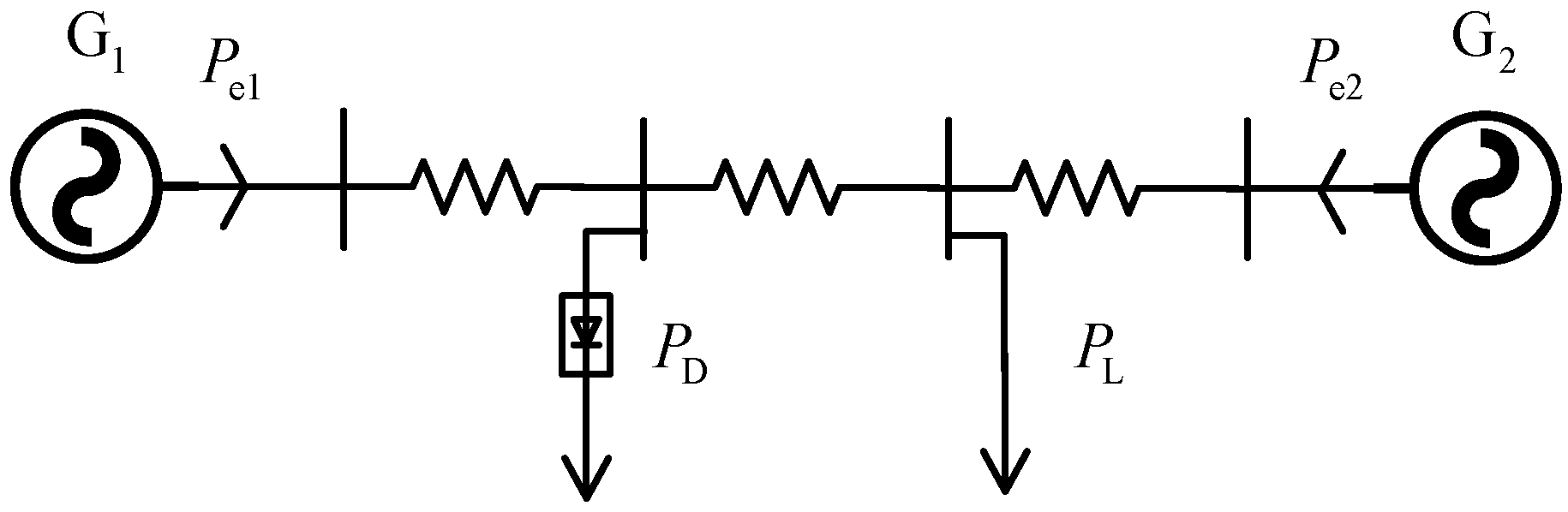
Figure 2.
Simulation results of CF.

Figure 3.
Chain of fault events.
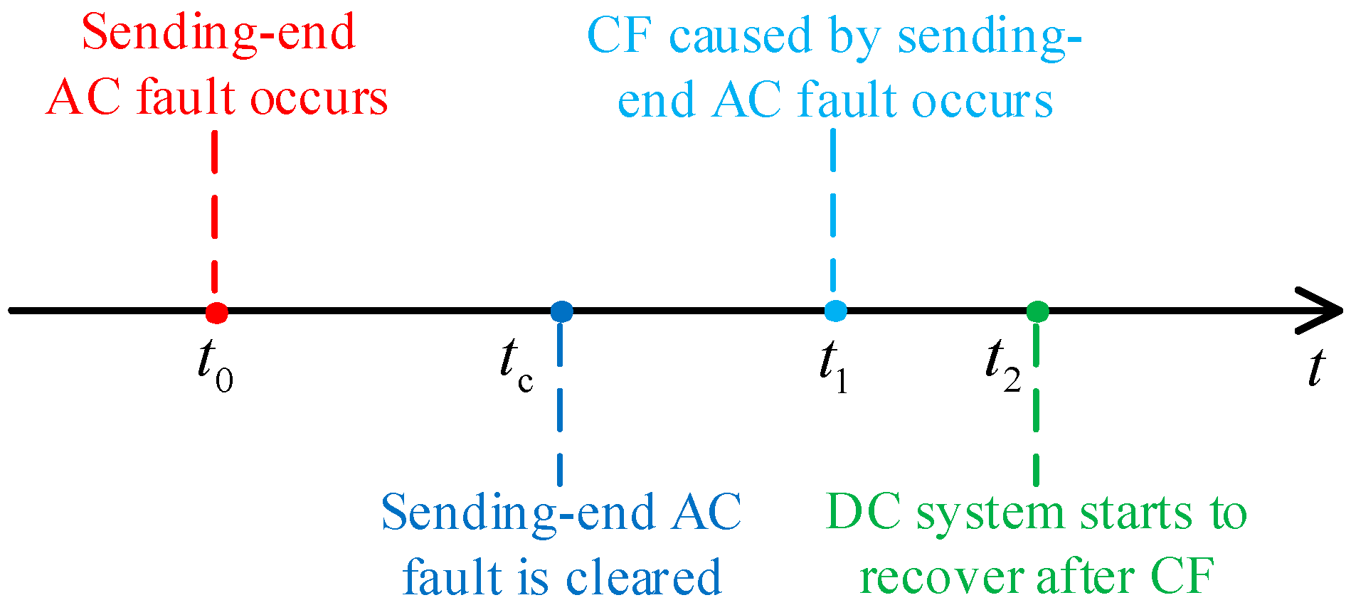
Figure 4.
Swing direction of relative rotor angle when the sending-end fault occurs.

Figure 5.
Equivalent reactance diagram of the sending-end power system.
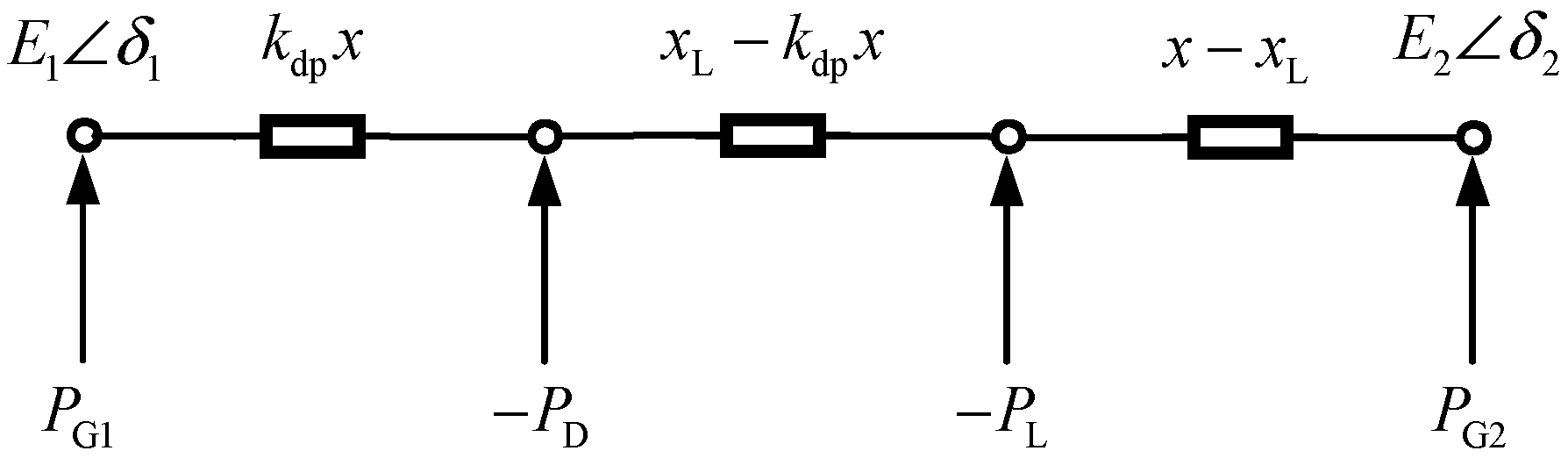
Figure 6.
Impact of CF on the TSSPS: (a) swing forward; (b) swing backward.
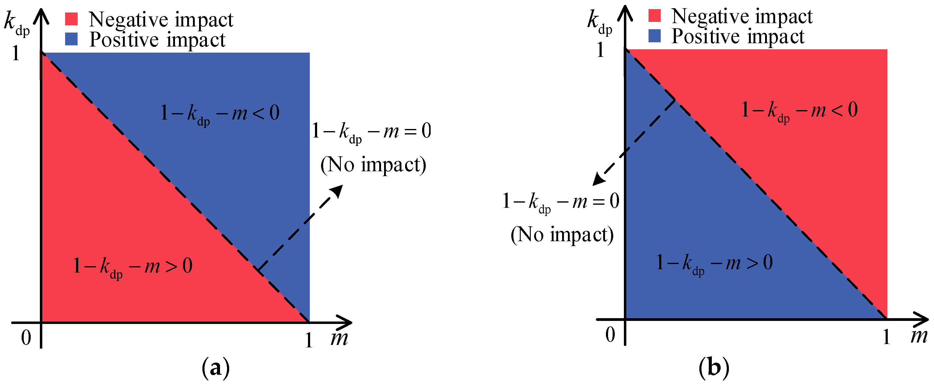
Figure 7.
Impact of improving the DC power recovery speed on the TSSPS: (a) swing forward; (b) swing backward.
Figure 7.
Impact of improving the DC power recovery speed on the TSSPS: (a) swing forward; (b) swing backward.

Figure 8.
Mathematical model of VDCOL.
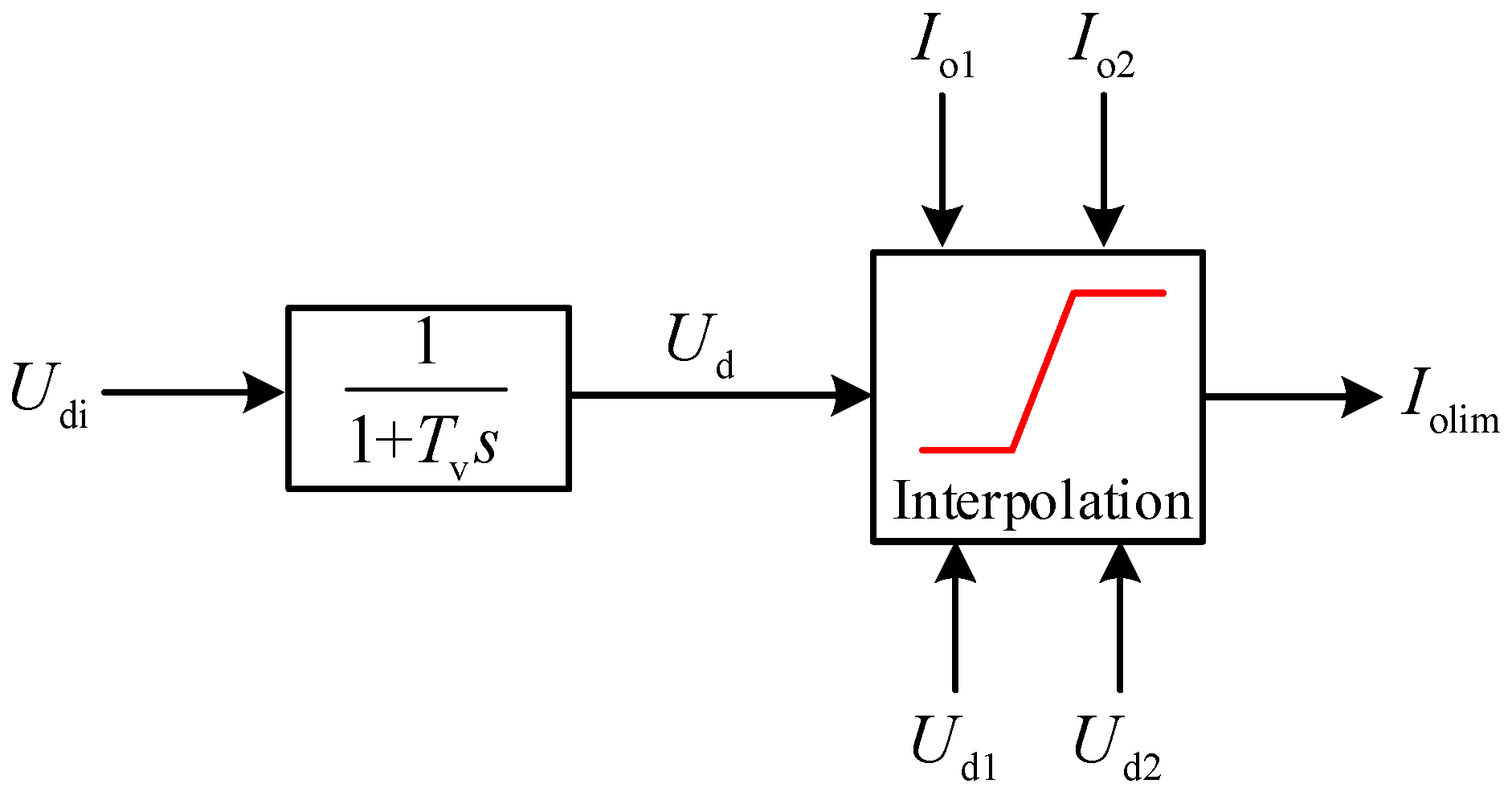
Figure 9.
Parameters of VDCOL: (a) changes; (b) changes.
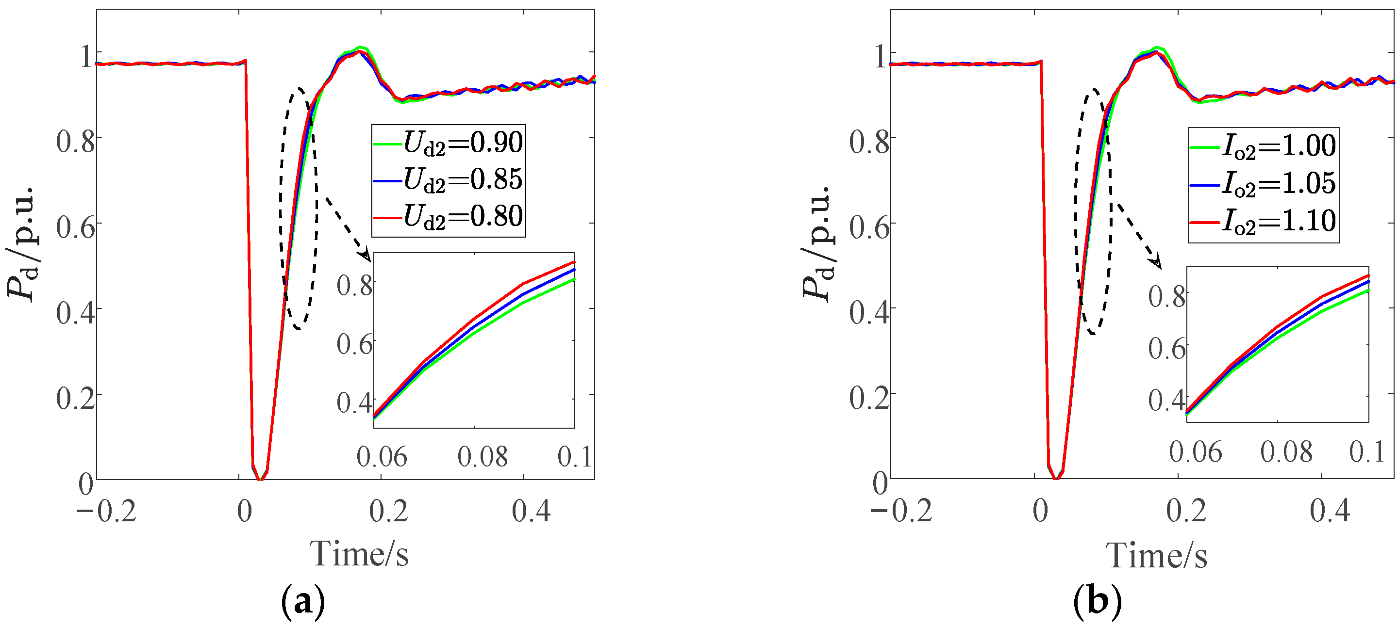
Figure 10.
Kundur’s two-area-based test power system.
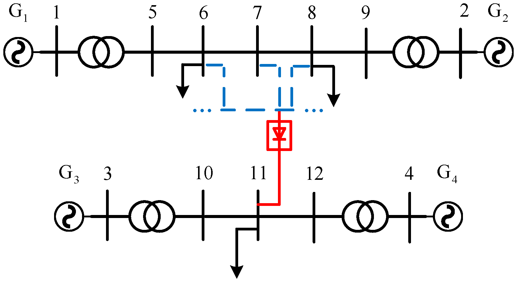
Figure 11.
Impact of CF on the TSSPS: (a) swing forward; (b) swing backward.
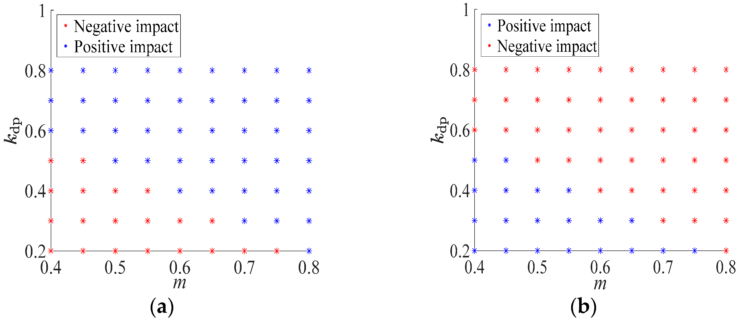
Figure 12.
Impact of increasing on the TSSPS: (a) swing forward; (b) swing backward.
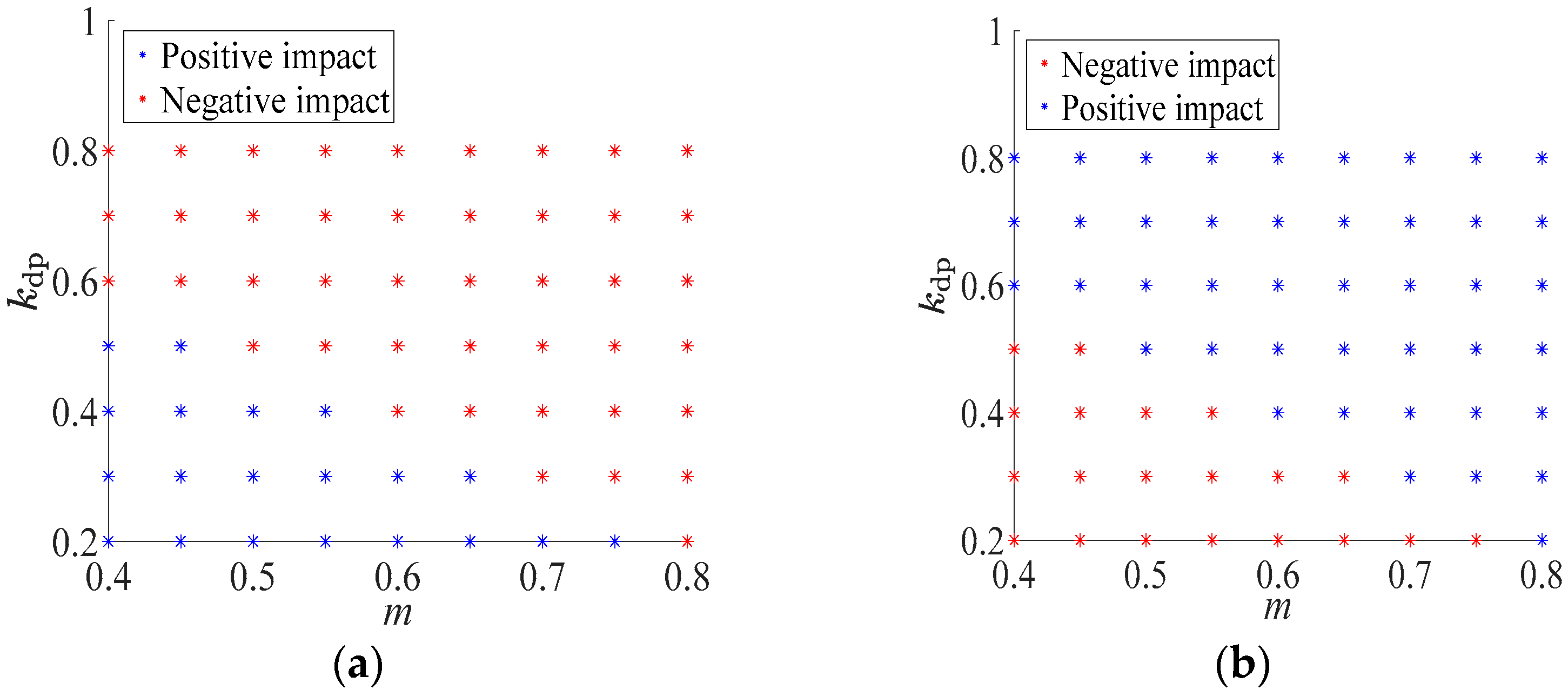
Figure 13.
IEEE 68-bus-based test power system.

Figure 14.
Scenario I: (a) relative rotor angle; (b) DC power.
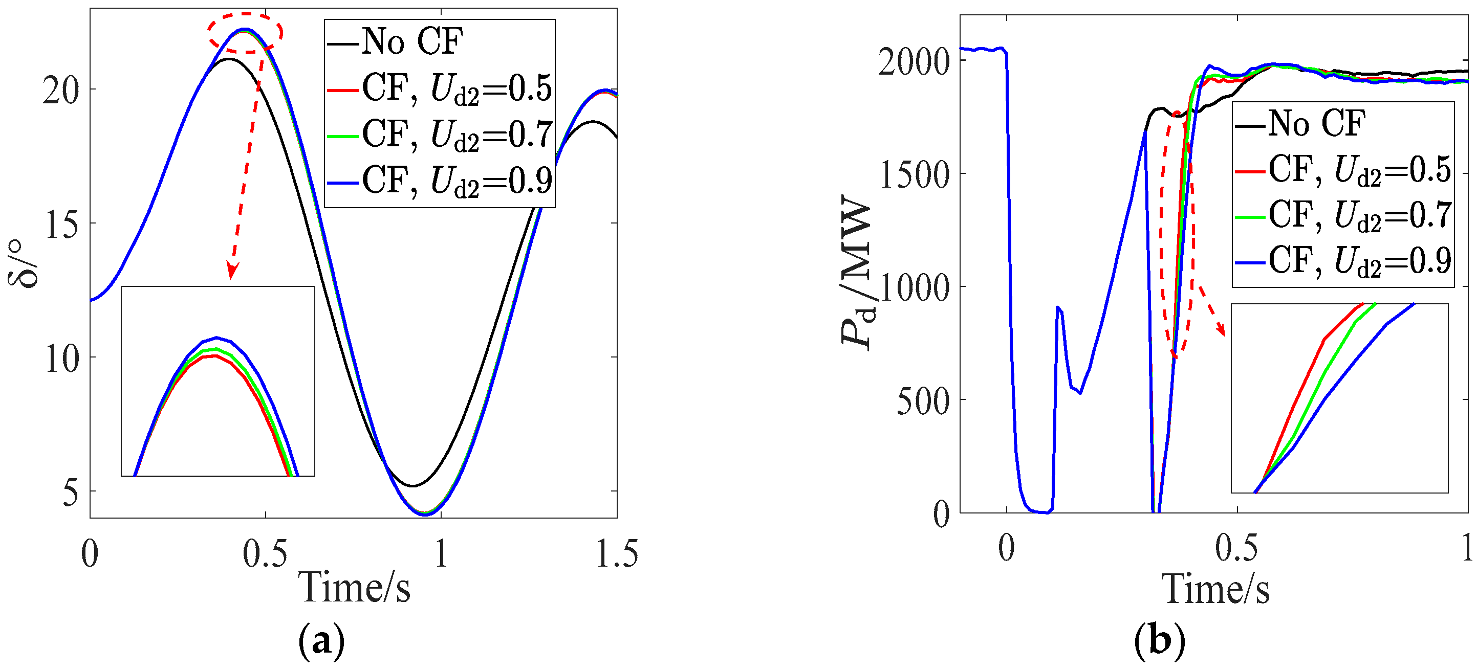
Figure 15.
Scenario II: (a) relative rotor angle; (b) DC power.
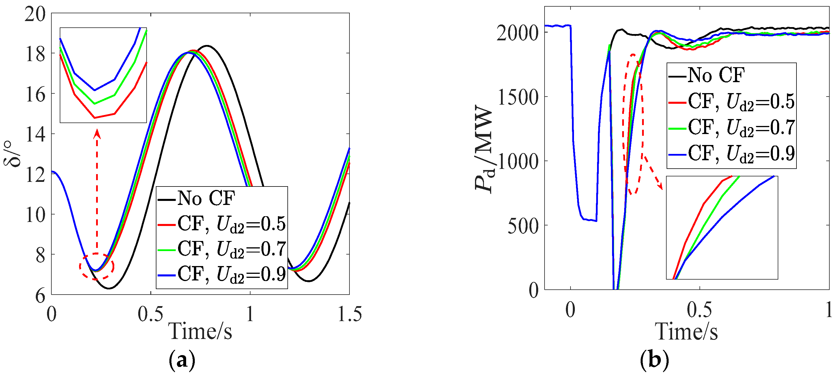
Figure 16.
Scenario III: (a) relative rotor angle; (b) DC power.
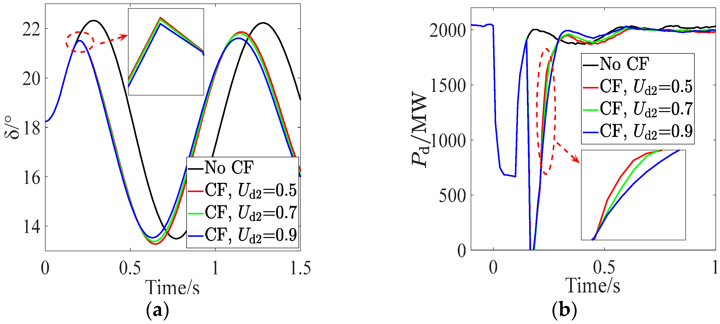
Figure 17.
Scenario IV: (a) relative rotor angle; (b) DC power.
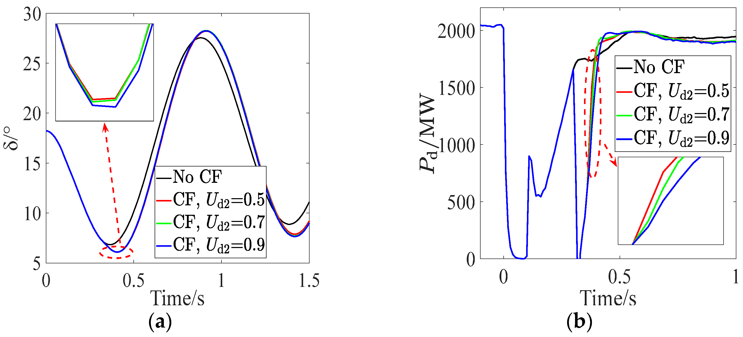
Figure 18.
Simulation results of different fault locations: (a) impact of CF on TSSPS; (b) impact of increasing on TSSPS.
Figure 18.
Simulation results of different fault locations: (a) impact of CF on TSSPS; (b) impact of increasing on TSSPS.
Disclaimer/Publisher’s Note: The statements, opinions and data contained in all publications are solely those of the individual author(s) and contributor(s) and not of MDPI and/or the editor(s). MDPI and/or the editor(s) disclaim responsibility for any injury to people or property resulting from any ideas, methods, instructions or products referred to in the content. |
© 2023 by the authors. Licensee MDPI, Basel, Switzerland. This article is an open access article distributed under the terms and conditions of the Creative Commons Attribution (CC BY) license (https://creativecommons.org/licenses/by/4.0/).
Share and Cite
MDPI and ACS Style
Lin, Y.; Hu, J.; Wang, T.; Wang, Z. Impact Mechanisms of Commutation Failure Caused by a Sending-End AC Fault and Its Recovery Speed on Transient Stability. Electronics 2023, 12, 3439. https://doi.org/10.3390/electronics12163439
AMA Style
Lin Y, Hu J, Wang T, Wang Z. Impact Mechanisms of Commutation Failure Caused by a Sending-End AC Fault and Its Recovery Speed on Transient Stability. Electronics. 2023; 12(16):3439. https://doi.org/10.3390/electronics12163439
Chicago/Turabian StyleLin, Yifeng, Jiawei Hu, Tong Wang, and Zengping Wang. 2023. "Impact Mechanisms of Commutation Failure Caused by a Sending-End AC Fault and Its Recovery Speed on Transient Stability" Electronics 12, no. 16: 3439. https://doi.org/10.3390/electronics12163439
Note that from the first issue of 2016, this journal uses article numbers instead of page numbers. See further details here.