
Quick Search Algorithm-Based Direct Model Predictive Control of Grid-Connected 289-Level Multilevel Inverter


1
Department of Electrical Engineering, University of Engineering and Technology, Lahore 54890, Pakistan
2
Clean and Resilient Energy Systems (CARES) Lab, Electrical and Computer Engineering Department, Texas A&M University, Galveston, TX 77553, USA
3
Department of Electrical Engineering, The University of Lahore, Lahore 54000, Pakistan
*
Authors to whom correspondence should be addressed.
Electronics 2023, 12(15), 3312; https://doi.org/10.3390/electronics12153312
Submission received: 26 June 2023
/
Revised: 25 July 2023
/
Accepted: 28 July 2023
/
Published: 2 August 2023
(This article belongs to the Special Issue Advanced Technologies in Power Electronics and Electric Drives)
Abstract
:Multilevel inverters, known for their low switching loss and suitability for medium- to high-power applications, often create a heavy computational overhead for the controller. This paper addresses the aforementioned limitation by presenting a novel approach to Direct Model Predictive Control (DMPC) for a grid-tied 289-level ladder multilevel inverter (LMLI). The primary objective is to achieve perfect inverter current control without enumeration. The proposed control method provides a single best solution without complete exploration of the search space. This generalized method can be applied to any multilevel inverter (MLI), enabling them to be used in the grid-tied mode without the computational burden due to a large number of switching states. The DMPC of LMLI with 289-level output and corresponding 289 control inputs, utilizes a discrete model to predict the future state of the state variable. In order to alleviate the enumeration burden, virtual sectors on a linear scale are introduced, and a general formula is provided to identify the single best state among the 289 states, reducing the time required to find the best optimal state per sampling period. Moreover, the proposed control scheme is independent of objective evaluation.
1. Introduction
The integration of clean and sustainable energy resources has significantly reduced reliance on fossil fuels, paving the way for greener and more environmental friendly power generation [1]. Grid-tied inverters play a central role in connecting distributed energy sources with the grid. In applications where the grid is connected, inverters are required to maintain voltage levels while keeping the total harmonic distortion (THD) to a minimum [2]. Additionally, they must provide the sinusoidal current waveform, adhering to the limit of total demand distortion (TDD) posed by IEEE 519-2022 [3].
Inverters that have fewer voltage levels in output employing advanced pulse width modulation (PWM) techniques such as space vector PWM produce high-quality current waveforms. However, these inverters encounter difficulties such as electromagnetic interference and increased voltage across switches in off-state. Moreover, each stage of voltage transformation in a power electronic system tied to the grid reduces its efficiency [4].
Multilevel inverters (MLIs) have become increasingly popular for generating high voltage from renewable sources because they offer the advantage of avoiding the complex designs of high-frequency transformers. On the other hand, MLIs, by employing a greater switch count to get sinusoidal output voltage, effectively decrease voltage across individual switches and ensure high-quality injected current. This makes MLIs highly suitable for demanding high-power applications where power quality is of utmost importance. Additionally, MLIs are well-suited for grid-tied and islanded systems that employ large battery banks [5]. However, this advancement requires difficult power control schemes to be implemented [6,7]. The power transfer from distributed energy sources to conventional grids heavily relies on the effective control of grid-tied inverters [8]. In grid-connected applications, achieving perfect reference tracking through current controllers is of paramount importance [9]. Many continuous control techniques are used in the literature to operate MLIs.
The utilization of a PI controller for power flow control of MLI, with certain switches operating at the fundamental frequency and the rest at the switching frequency, has been proposed by [2,10]. To tune the gains of the PI controller, meta-heuristic algorithms such as Firefly (FF), Harris Hawk (HH) and Particle Swarm Optimization (PSO) are employed, in addition to calculating the switching angles for SHE-PWM as discussed in [11,12]. Furthermore, control techniques that employ a system model are applied in conjunction with innovative PWM techniques, which are presented in [13,14]. However, the above techniques cannot handle constraints and non-linearities and always require a modulator to generate pulses for controlling switches. Moreover, modern systems may not have a single underlying objective; rather, objectives can consist of multiple parts which is impossible with the conventional linear controllers.
To address these challenges, model predictive control (MPC) has emerged as a promising solution in recent times [15]. MPC offers several attractive features, such as rapid dynamic response, obviating the requirement for modulators, consolidation of multiple nested control loops into a single loop, and the ability to accommodate system requirements in diverse disciplines [16,17,18,19,20]. However, MPC for MLIs suffers from a high computational burden due to a large number of switching devices to be controlled [21]. MPC uses a small sampling period to track the state variable properly. However, a small sampling time means less time for computations. One possible way to solve this issue is to solve the problem offline, save the control input in the lookup table, and apply values from the lookup table when the online operation is desired [22,23]. However, the obvious limitation of this method is the absence of disturbance control. The controller can only know about a disturbance after it happens. So, this approach will fail in practical situations. In [21], MPC is used to control cascaded H-Bridge. Due to the 125 total number of permissible voltage vectors, only adjacent seven vectors are used to reduce the computations, but this comes at the expense of setting a trade-off between performance and speed. Moreover, voltage levels are not practical and do not meet the THD limit for grid-tied operation. Reference [24] converts the current control problem to voltage control, thereby avoiding the search for optimal state among 512 states, but this is not a generalized method since many MLIs come with hundreds of different voltage levels, so even after finding a reference voltage, a search burden follows. In [25], another technique is based on reference voltage extraction. It divides the search space into 96 triangles, each having three vectors. The voltage prediction results in the selection of a single triangle, but due to offline calculation, the information related to demand change needs to be embedded; therefore, it may fail in practical situations. In [26,27], the above technique has been used resulting in 26 and 24 triangles, respectively, but it suffers from memory issues since it needs to use look-up tables. Moreover, finding one triangle is difficult, and the technique needs to be more generic. A further reduction in triangles is done by [28], where reduction up to 16 from 96 triangles is done. All the above techniques apply to MLIs that exploit the state space structure. A particular sector can be identified based on real and imaginary voltage components. However, this privilege is available only with the inverters in a three-phase topology. Moreover, besides making the current sinusoidal, the THD of voltage must be maintained, which should be mentioned in the above studies.
In [29], a heuristic is built for packed U-cell MLI for finding optimal state locations. However, the method does not work for other MLIs with a different number of levels and different topology. Moreover, the second objective is ignored while searching for a state. In [30], another simplification is proposed for single-phase MLI without objective evaluation, but complex analysis has to be performed to develop this control for other topologies. In [14], MPC controls single-phase MLI by enumerating all possible switching states. It may result in a large delay while applying the control signal that deteriorates the performance of state variables. There is a lack of literature on controlling single-phase MLI with MPC [31]. Much effort has been put into proposing new techniques in terms of MLI topologies. These studies are done to reduce switch count with increased voltage levels, improved transient response, lower number of capacitor balance circuits and level of modularity. The interested readers are referred to read [12,32,33,34,35,36,37,38,39,40,41,42].
The main emphasis of the mentioned research revolves around addressing control issues related to three-phase inverter topologies and the advancement of novel MLI configurations that optimize the utilization of switching devices and input sources. However, the exploration of power injection control strategies into the grid remains relatively limited within the scope of this study.
The major contributions as compared to traditional DMPC of LMLI are listed as follows:
- A Quick Search Algorithm (QSA)-based Direct Model Predictive Control (DMPC) technique, enabling the calculation of the single best switching state without the need to search the entire state space exhaustively.
- Proposed a technique independent of objective evaluation during each sampling interval, reducing computational complexity.
- Generalized the new technique to apply to any MLI, expanding its versatility and applicability.
- The computational burden associated with traditional DMPC methods for MLIs is addressed. The new proposal offers improved computational efficiency.
- Demonstrated the capability of the proposed control method to generate lower compared to traditional DMPC techniques.
- Established the robustness of the proposed control scheme under step disturbances in power demand and filter parameter variations.
The paper is organized as follows: Section 2 describes the operating principle of single-phase 289-level LMLI, Section 3 presents the modeling of the 289-level grid-connected LMLI, Section 4 presents the DMPC of 289-level LMLI, Section 5 presents the simulation results, and Section 6 concludes the paper with Discussion.
2. Operation of 289-Level Ladder Multilevel Inverter (LMLI)
The operational details of the 289-level LMLI are depicted in Figure 1, following the approach described in [43]. It consists of two units of LMLIs connected in series. There are four bidirectional switches and twelve unidirectional switches . Additionally, it consists of eight independent power supplies, which can consist of either four or eight voltage levels, depending on the desired symmetry. While an alternative technique utilizing a single input dc with voltage divider has been proposed in [35], practical implementation encounters challenges in voltage balancing across the capacitor, necessitating the use of voltage balancing circuits [10]. This study investigates the control of LMLI in a grid-tied environment using separate DC sources. The term “ladder” is derived from the bidirectional switches that facilitate bidirectional power flow. The 289 allowed switching states can be found in Table 1. Figure 1 depicts the connection of the LMLI to a grid through an filter. By configuring the inverter with the specified power supplies, a 289-level output is achieved, where “1” indicates a switch in conduction mode, and “0” represents an open switch state.
Using the following supply voltages for eight sources in Figure 1, all 289-voltage levels can be achieved by employing allowable switching combinations from Table 1. By choosing a suitable value of , any peak-to-peak or rms value of output voltage can be achieved. However, in a recent study [44], a meta-heuristic method such as Dragonfly is used to optimally select the voltage sources.
and
The peak values of voltages are and . The voltage difference in any two consecutive output voltage levels is on both positive and negative sides.
3. Modeling of Grid-Connected 289-Level LMLI
The system being investigated can be represented using its equivalent differential equation description, as expressed in Equation (1). Figure 1 illustrates the connection of the grid to an inverter through a series -filter. The current injected into the grid as “”, the inverter voltage as “” and grid voltage is denoted as “”.
As digital systems inherently operate on discrete values, the discretization of Equation (1) has been performed using the Euler method with a sampling period denoted as . Thus, Equations (1) and (2) can be represented in the following manner:
In Equation (4), is the predicted current value for a single-phase system. The , and are measured single-phase voltage and current at kth instant. Given the sensory measurements and permissible values of “”, prediction of current can be made for the next sampling instant using Equation (4).
4. DMPC of 289-Level LMLI
DMPC (Direct Model Predictive Control) is a model-based control strategy that leverages the system’s model to forecast future values. These predicted values guide the determination of the control input in real-time. Given the significance of current control, both in terms of magnitude and quality, in grid-tied applications, Equation (4) can be employed to anticipate future grid current values.
In traditional DMPC approach, the inverter voltage is chosen based on the 289 states outlined in Table 1. Subsequently, an objective function is employed to determine the optimal voltage input, allowing for the evaluation of each state from the 289 available options. The state that has been determined as the most optimal is subsequently implemented at the k-th moment. The objective to account for current deviation can be defined in the following manner:
In the case of extremely small sampling times, such as 20 s, it can be assumed that the reference current remains relatively constant within each sampling interval. Consequently, one can infer the following:
However, when dealing with larger sampling intervals, such as 100 , relying solely on the aforementioned assumption would result in predictions that deviate from the reference [16]. As a consequence, this can lead to increased current ripples and a degradation in current quality. Consequently, the application of an extrapolation method becomes necessary to address this issue.
4.1. Extrapolation
The first benefit of three-phase to frame conversion is to manipulate the angular displacement of the rotating vector to extrapolate the current value. Besides this, there is no need to store the past value; only the present value (assuming the magnitude remains constant) can be used. In addition, this method outperforms Lagrange’s extrapolation method for tracking sinusoidal values [16]. The idea is to shift the current vector forward with the help of angular displacement using the magnitude of the present sample as shown in Figure 2.
The general formula for future projection is given as follows:
where “n” refers to the future sample whose prediction is required. Using this method, the future value of any variable for th and th instant can be found using their present value as follows:
By using Equation (15), the can be extrapolated.
4.2. Delay Compensation for DMPC
Ideally, calculating the best voltage vector for each sampling instant takes little time, and the new best switching state is instantly calculated and applied simultaneously. However, practically, it is not possible. It is dependent on the processing speed of the microprocessor. In most practical scenarios, when massive calculations are made during each sampling instant, a controller delay is always there, as reported in [45], due to which the predicted value does not follow the reference and ripple increases. If calculations take half a sampling period to calculate the new switching state, then the old state will continue to be applied for that half sampling time. The new state will be applied after half of the sampling period. Therefore, the controller will be unable to track the reference, and oscillations will increase. To address this issue, a delay compensation technique has been proposed by [16]. At the start, optimal switching state is applied, and then using the corresponding inverter voltage, the inverter current is estimated for th instant. Using estimated current, projected values of grid voltage and measured current at th instant, the current fed to the grid is predicted for th instant. For single-phase system, estimated current at th instant can be represented as:
with being the estimated current injected in the grid at th instant, and using this predicted value, the next instant can be predicted as:
In Equation (17), is the extrapolated value of grid voltage obtained through extrapolation, and is the inverter voltage selected among 289-values and the state corresponding to that voltage will be applied in the next sampling instant.
The objective function given in Equation (5) for a single-phase system can be updated as follows:
where is the extrapolated reference current given below:
The problem of delay in applying the control signal due to calculations is minimized. However, the number of states is 289, and the controller is required to check every input at each sampling period.
4.3. QSA Based DMPC
The proposed DMPC takes a start from the objective function. Let us consider that at th–instant, the inverter current is perfectly equal to the reference current, then:
By substituting in Equation (17), the new dynamic equation can be written as:
From Equation (23), it can be deduced that the inverter voltage , is the expected reference voltage that made the inverter current equal to the reference current. Therefore,
Now, Equation (23) can be further updated as follows:
Using Equation (26), there is no need to evaluate the objective function at every sampling instant because the inverter voltage that will make the injected current equal to the reference current has been found. Thus, the proposed DMPC is independent of the objective function due to the reformulation of the control problem in terms of inverter voltage instead of current. However, this is not of much significance since there are 289 distinct voltage values, among which one close to the derived reference voltage must be chosen.
By exploiting the sign of the reference inverter voltage , the search space can be divided into two parts with positive and negative voltages, hence reducing the number of states to be searched to half (i.e., 144 along with a common zero state). However, the search space is still enormous for a small sampling interval. Moreover, with three cascaded topologies of LMLI, there are total states. So, even dividing in half only works for a small number of voltage levels reaching hundreds and thousands. So, a general method is missing in the literature that can be used to search for the best state closest to the reference voltage through any given number of states.
The proposed QSA starts by virtually dividing the search space into sectors on a linear scale. Each linear sector spans a voltage range of “” in magnitude. By suitably selecting the value of , one can achieve desired peak-to-peak voltage at the output. The Figure 3 shows the sectors on x-axis and corresponding to each sector there is a state shown in shaded area and y-axis. Each state dictates the voltage up to the middle of the previous to the middle of next sector, thus resulting in the following configuration:
with being the state that produces zero voltage. The variable “k” corresponds to the index of state which will be applied to switches and there is a unique voltage value that appears as the output of inverter corresponding to each state. Now, one can find states corresponding to each voltage reference produced. However, this method could result in a lookup table that eats up memory. So, a general rule has been developed by dividing with and taking the quotient. Now, adding “1” to the result produces the sector number where the reference voltage lies. Then,
where “n” is the sector number. Nevertheless, this sector number is different from the states that are available to be applied. This sector number has to be translated to the corresponding state number.
However, there is no direct relation between sector and switching state, because every switching state covers two sectors. From Figure 3, the following results can be deduced:
By building intuition from Equations (32)–(35), one can generalize the relation between sectors and corresponding state to be applied as follows:
Otherwise,
where “” represents the set of integers and “k” is the state number that can be applied to the inverter at th-instant. This time, irrespective of the number of levels, only one state is obtained that needs to be applied without evaluating the objective function. The complete pseudo code for proposed QSA based DMPC is given in Algorithm 1.
| Algorithm 1: QSA based DMPC |
 |
The conventional DMPC poses a huge computational burden because, in every sampling interval, all 289 states have to be spanned to find one that minimizes the tracking error of the state variable with respect to the reference. However, the proposed method can reduce the number of states to only one per sampling interval. MLI’s benefits can be availed in low THD applications pragmatically since processing speed is a big issue in model-based predictive control schemes. A complete block diagram of QSA based DMPC is given in Figure 4. The objective function block is given the value of grid voltage “” because it is required to make predictions about the state variable as given in Equations (5) and (25).
5. Simulation Results
It is very crucial to use a model that is valid for pragmatic purposes because otherwise the model-based control approaches may result in useless results, causing the system to lose its stability in online operation. The model used in this study has been used by various researchers in the field of model predictive control for power electronics [2,10,11,14,45,46,47,48]. The validity of the results can be readily confirmed by simulating the 289-level LMLI in MATLAB Simulink. To demonstrate the practicality of the proposed DMPC scheme based on the QSA, an LMLI is connected to the grid in a single-phase arrangement. A sampling time of 24 is employed to simulate the novel control scheme. The grid has a voltage of 230 V at 50 Hz frequency. The filter resistance is and two different values for inductance 12 mH and 2 mH, are used. The subsequent sections explain the steady-state, dynamic, parametric variation effect and response of the 289-level LMLI under grid-connected condition. Moreover, it is essential to note that increasing the number of switches in the circuit comes with the difficulty of increasing the number of switching combinations. MLI with output current and voltage approaching closely to sinusoidal suffers a high computational burden. However by using the proposed technique, this time can be utilized by the computational resources to perform other calculations such as processing analog to digital converter’s data, etc.
5.1. Steady-State Performance of 289-Level LMLI
Figure 5 and Figure 6 present the voltage and current waveforms of the grid-tied 289-level LMLI under steady-state conditions. The magnitude and frequency of the output voltage align with those of the grid. Furthermore, the current waveform exhibits a pure sinusoidal shape, with a total harmonic distortion (THD) of , meeting the IEEE’s THD limit of 5%. Harmonic analysis, as depicted in Figure 7 and Figure 8, illustrates the injection of 1 kW power into the grid, resulting in a current magnitude of 6.15A for two different inductance values. Given the remarkably low THD of the current, this system is well-suited for standalone and grid-connected environments featuring renewable energy sources as excitation. Moreover, the single-phase and three-phase topologies of two-level inverters suffer the high harmonic content in voltage signals and thus require filters. However, filters come with stability issues; more specifically, LCL filter has a significant drawback in terms of resonance. In order to deal with resonance, either active damping or digital filters must be used. However, the LMLI has no such problem. Using a few more switches, the voltage waveform is pure sinusoidal, and THD, as shown in Figure 7a and Figure 8a is only , which is negligible and makes LMLI a perfect candidate for grid-tied applications. It must be noted that Figure 7 and Figure 8 are drawn without the fundamental component of voltage and current to show the magnitude of harmonics present in the spectrum effectively.
5.2. Dynamic Response of 289-Level LMLI
Achieving a grid that remains completely immune to disturbances, such as load variations, poses a significant challenge. When the inverter is supplying power to the grid, it becomes essential to assess its performance under sudden changes in power demand and parametric variations, which can occur due to factors such as temperature fluctuations affecting the DC resistance of the inductor. To observe the fast dynamic response of the proposed DMPC, Figure 9 and Figure 10 demonstrate the step changes applied to the reference current of the 289-level LMLI. The active power is modified from 1 kW to 2 kW at 35 ms and remains constant at 2 kW until 85 ms, after which it is reverted back to 1 kW. This test allows for the assessment of the system’s performance when subjected to changing load conditions.
In grid-tied applications, the control action of the inverter must be readily adaptable to demand changes, as the load demand on the grid continuously fluctuates, directly impacting the power requirements from renewable sources connected to the grid. To assess the system’s response to sudden demand changes, Figure 11 and Figure 12 provide a focused view of the voltage and current waveforms for both step-up and step-down scenarios. Specifically, Figure 11a,b zoom in on the step applied at 35 ms, with the highlighted region showcasing the convergence of the inverter voltage and output current towards their respective reference waveforms. Remarkably, the voltage and current injected into the grid took only 1.4 ms to align with new current demand, underscoring the rapid dynamic response of the proposed QSA-based DMPC approach. There is an important conclusion to draw from dynamic response that not only the control system but the value of the inductor also considerably affect the performance of the system during disturbances. So, it is suggested to carefully choose the value of the inductor for grid-tied applications. It can be seen from Figure 9a,b, that for smaller value of inductor (L = 2 mH), there is considerable increase in the , although both values of inductance work well in steady-state operation.
Furthermore, as depicted in Figure 12a,b, it is evident that the step decrease in reference current demand introduced at 85 ms has minimal impact on the control response. Both the inverter voltage and current accurately track the reference with an insignificant time delay of 0.32 ms and 0.15 ms, respectively, which is even shorter compared to the step-up scenario.
5.3. Effect of Parametric Variation
The filter parameters are added to model the effect of the inductor’s internal resistance, which varies with temperature. As the temperature rises, it also rises. The same is the case for inductance value because permeability is also dependent on temperature. So, in order to emulate this kind of behavior, the step change in inductance is utilized without providing any information to the model of system to examine the impact of temperature-induced changes in inductance on controller performance.
Figure 13 and Figure 14 illustrate the voltage and current behavior during online operation when a step change is applied to the filter inductance. In the worst-case scenario, a 50% step-up change is implemented by adjusting the inductance from 12 mH to 18 mH from 30 ms to 60 ms. Subsequently, a step-down change from 12 mH to 6 mH occurs from 90 ms to 150 ms for the 289-level LMLI. Throughout the inductance variation, the power remains constant at 1 kW. Figure 14 illustrates the behavior of the LMLI current, which demonstrates a remarkable ability of the controller to closely track the reference signal without any discernible oscillation or deviation, thereby preserving a pristine sinusoidal waveform.
5.4. Reduced with Proposed DMPC
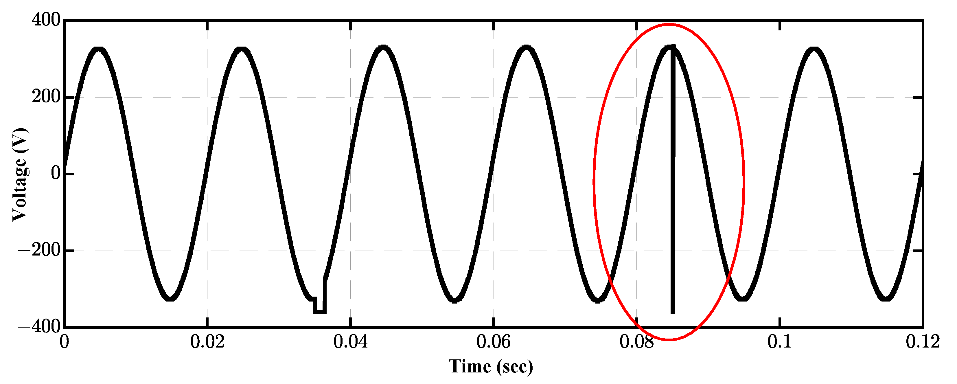
By conventional DMPC, the inverter output voltage has a very high change in voltage per sampling interval, as visible in Figure 15. The control input has been transitioned from a positive peak to a negative peak in one sampling interval to make the inverter current follow the reference as quickly as possible. However, this adverse effect can damage switches and cross the load voltage limit connected at the point of common coupling.
However, in the proposed method, whenever a significant transition of voltage is detected, instead of applying input directly, it is applied in steps with increasing magnitude in successive steps as shown in Figure 12a, thus avoiding the high .
6. Discussion
In this paper, a novel QSA-based Direct Model Predictive Control (DMPC) technique for a 289-level grid connected ladder multilevel inverter (LMLI) has been presented. The QSA has significantly reduced the search burden by efficiently calculating the single best state to be applied at the th instant. The new control scheme eliminates the need for exhaustive state enumeration and significantly improves computational efficiency. Additionally, the proposed technique eliminates the requirement for objective function evaluation for each state, further streamlining the control process. The QSA-based DMPC technique presented in this study is generalized and can be applied to any MLI with any number of voltage levels. This flexibility makes it highly suitable for grid-connected applications, providing a single-state solution for various MLIs. Model-based predictive current control techniques, particularly for MLIs, typically involve substantial computation time. The proposed technique has demonstrated a substantial reduction in search time compared to conventional DMPC methods, which is of significant practical importance.
The Total Harmonic Distortion (THD) limits for current and voltage were found to be and , respectively, which is negligible and well below the standard IEEE limit of for a 289-level LMLI. The proposed controller has exhibited perfect steady-state operation with sinusoidal current and voltage waveforms. Its fast dynamic response ensures stable operation under changing demand conditions. Moreover, the controller has demonstrated robustness to filter parameter variations and low , further enhancing its practical applicability. Considering these characteristics, the DMPC-based 289-level LMLI, incorporating the proposed QSA algorithm, is highly suitable for high-power standalone and grid-connected applications.
Future works will include the voltage control of DC links. Most studies use only a single DC-link capacitor at the input. However in this case, there are a total of eight different voltage supplies. Further studies will also contain a complete PV installed in a rural area system with MPPT capability, including voltage control of complex setup in a DC microgrid where the LMLI will act as a bridge between the DC grid and AC grid. Moreover, the control system will be tested under dynamic load variation conditions, so that transient behavior can be analyzed and improved.
Author Contributions
Conceptualization, M.A.B. and S.A.R.K.; methodology, M.A.B. and S.A.R.K.; software, M.A.B., S.A.R.K. and I.A.K.; validation, M.A.B., I.A.K. and G.A.; formal analysis, M.A.B., I.A.K. and G.A.; investigation, M.A.B. and G.A.; resources, S.A.R.K.; data curation, M.A.B., I.A.K.; writing—original draft preparation, M.A.B. and S.A.R.K.; writing—review and editing, M.A.B., I.A.K. and G.A.; visualization, M.A.B., S.A.R.K. and I.A.K.; supervision, S.A.R.K.; funding acquisition, S.A.R.K., I.A.K. and G.A. All authors have read and agreed to the published version of the manuscript.
Funding
This research received no external funding.
Institutional Review Board Statement
Not applicable.
Informed Consent Statement
Not applicable.
Data Availability Statement
Not applicable.
Acknowledgments
The authors would like to acknowledge the support of Power Systems Simulation Research Laboratory (PSSRL) at the Department of Electrical Engineering, University of Engineering and Technology, Lahore. The computational resources of the PSSRL were used in this research.
Conflicts of Interest
The authors declare no conflict of interest.
References
- Nwaigwe, K.N.; Mutabilwa, P.; Dintwa, E. An overview of solar power (PV systems) integration into electricity grids. Mater. Sci. Energy Technol. 2019, 2, 629–633. [Google Scholar] [CrossRef]
- Sayed, M.A.; Elsheikh, M.G.; Orabi, M.; Ahmed, E.M.; Takeshita, T. Grid-Connected Single-Phase Multi-Level Inverter. In Proceedings of the 2014 IEEE Applied Power Electronics Conference and Exposition-APEC 2014, Fort Worth, TX, USA, 16–20 March 2014; pp. 2312–2317. [Google Scholar]
- 519-2022; IEEE Standard for Harmonic Control in Electric Power Systems. IEEE: Piscataway, NJ, USA, 2022. [CrossRef]
- Oliveira, K.C.; Afonso, J.L.; Cavalcanti, M.C. Multilevel inverter for grid-connected photovoltaic systems with active filtering function. IFIP Adv. Inf. Commun. Technol. 2013, 394, 289–298. [Google Scholar] [CrossRef] [Green Version]
- Adefarati, T.; Bansal, R.C. Integration of Renewable Distributed Generators into the Distribution System: A Review. IET Renew. Power Gener. 2016, 10, 873–884. [Google Scholar] [CrossRef]
- Carrasco, J.M.; Franquelo, L.G.; Bialasiewicz, J.T.; Galván, E.; Portillo Guisado, R.C.; Prats, M.Á.M.; León, J.I.; Moreno-Alfonso, N. Power-electronic systems for the grid integration of renewable energy sources: A survey. IEEE Trans. Ind. Electron. 2006, 53, 1002–1016. [Google Scholar] [CrossRef]
- Sajadian, S.; Ahmadi, R. Model predictive control of dual-mode operations Z-source inverter: Islanded and grid-connected. In Proceedings of the 2017 IEEE Energy Conversion Congress and Exposition (ECCE), Cincinnati, OH, USA, 1–5 October 2017; pp. 4971–4977. [Google Scholar] [CrossRef]
- Azab, M. A finite control set model predictive control scheme for single-phase grid-connected inverters. Renew. Sustain. Energy Rev. 2021, 135, 110131. [Google Scholar] [CrossRef]
- Huang, X.; Wang, K.; Fan, B.; Yang, Q.; Li, G.; Xie, D.; Crow, M.L. Robust Current Control of Grid-Tied Inverters for Renewable Energy Integration Under Non-Ideal Grid Conditions. IEEE Trans. Sustain. Energy 2020, 11, 477–488. [Google Scholar] [CrossRef]
- Priyadarshi, A.; Kar, P.K.; Karanki, S.B. Grid Integration of a Reduced Switching Loss Single-Source Boost Multilevel Inverter with Independent Control of Power Transfer and DC-Link Voltage. In Proceedings of the 2021 IEEE 12th Energy Conversion Congress & Exposition-Asia (ECCE-Asia), Singapore, 24–27 May 2021; pp. 1414–1419. [Google Scholar] [CrossRef]
- Shunmugham Vanaja, D.; Stonier, A.A. Grid integration of modular multilevel inverter with improved performance parameters. Int. Trans. Electr. Energy Syst. 2021, 31, e12667. [Google Scholar] [CrossRef]
- Jayakumar, T.; Ramani, G.; Jamuna, P.; Ramraj, B.; Chandrasekaran, G.; Maheswari, C.; Stonier, A.A.; Peter, G.; Ganji, V. Investigation and validation of PV fed reduced switch asymmetric multilevel inverter using optimization based selective harmonic elimination technique. Automatika 2023, 64, 441–452. [Google Scholar] [CrossRef]
- Amamra, S.A.; Meghriche, K.; Cherifi, A.; Francois, B. Multilevel Inverter Topology for Renewable Energy Grid Integration. IEEE Trans. Ind. Electron. 2017, 64, 8855–8866. [Google Scholar] [CrossRef] [Green Version]
- Satti, M.B.; Hasan, A.; Ahmad, M.I. A new multilevel inverter topology for grid-connected photovoltaic systems. Int. J. Photoenergy 2018, 2018, 9704346. [Google Scholar] [CrossRef] [Green Version]
- Trabelsi, M.; Bayhan, S.; Ghazi, K.A.; Abu-Rub, H.; Ben-Brahim, L. Finite-Control-Set Model Predictive Control for Grid-Connected Packed-U-Cells Multilevel Inverter. IEEE Trans. Ind. Electron. 2016, 63, 7286–7295. [Google Scholar] [CrossRef]
- Rodriguez, J.; Cortes, P. Predictive Control of Power Converters and Electrical Drives; Wiley: Hoboken, NJ, USA, 2012. [Google Scholar] [CrossRef]
- Zanchetta, P.; Cortes, P.; Perez, M.; Rodriguez, J.; Silva, C. Finite states model predictive control for Shunt active filters. In Proceedings of the IECON Proceedings (Industrial Electronics Conference), Melbourne, VIC, Australia, 7–10 November 2011; pp. 581–586. [Google Scholar] [CrossRef]
- Cortés, P.; Rodríguez, J.; Quevedo, D.; Silva, C. Predictive current control strategy with imposed load current spectrum. In Proceedings of the 2006 12th International Power Electronics and Motion Control Conference, Portoroz, Slovenia, 30 August–1 September 2006; Volume 23, pp. 252–257. [Google Scholar] [CrossRef]
- Rodriguez, J.; Pontt, J.; Silva, C.A.; Correa, P.; Lezana, P.; Cortes, P.; Ammann, U. Predictive Current Control of a Voltage Source Inverter. IEEE Trans. Ind. Electron. 2007, 54, 495–503. [Google Scholar] [CrossRef]
- Rodriguez, J.; Cortes, P.; Kennel, R.; Kazmierkowski, M.P. Model predictive control - A simple and powerful method to control power converters. In Proceedings of the 2009 IEEE 6th International Power Electronics and Motion Control Conference, Wuhan, China, 17–20 May 2009; pp. 41–49. [Google Scholar] [CrossRef]
- Cortes, P.; Wilson, A.; Kouro, S.; Rodriguez, J.; Abu-Rub, H. Model predictive control of multilevel cascaded H-bridge inverters. IEEE Trans. Ind. Electron. 2010, 57, 2691–2699. [Google Scholar] [CrossRef]
- Beccuti, A.G.; Mariéthoz, S.; Cliquennois, S.; Wang, S.; Morari, M. Explicit model predictive control of DC-DC switched-mode power supplies with extended kalman filtering. IEEE Trans. Ind. Electron. 2009, 56, 1864–1874. [Google Scholar] [CrossRef]
- Cychowski, M.; Szabat, K.; Orlowska-Kowalska, T. Constrained model predictive control of the drive system with mechanical elasticity. IEEE Trans. Ind. Electron. 2009, 56, 1963–1973. [Google Scholar] [CrossRef]
- Xia, C.; Liu, T.; Shi, T.; Song, Z. A Simplified Finite-Control-Set Model-Predictive Control for Power Converters. IEEE Trans. Ind. Inform. 2014, 10, 991–1002. [Google Scholar] [CrossRef]
- Kim, I.; Chan, R.; Kwak, S. Model predictive control method for CHB multi-level inverter with reduced calculation complexity and fast dynamics. IET Electr. Power Appl. 2017, 11, 784–792. [Google Scholar] [CrossRef]
- Yang, Y.; Wen, H.; Fan, M.; Xie, M.; Chen, R. Fast Finite-Switching-State Model Predictive Control Method Without Weighting Factors for T-Type Three-Level Three-Phase Inverters. IEEE Trans. Ind. Inform. 2019, 15, 1298–1310. [Google Scholar] [CrossRef]
- Mora, A.; Cárdenas-Dobson, R.; Aguilera, R.P.; Angulo, A.; Donoso, F.; Rodriguez, J. Computationally Efficient Cascaded Optimal Switching Sequence MPC for Grid-Connected Three-Level NPC Converters. IEEE Trans. Power Electron. 2019, 34, 12464–12475. [Google Scholar] [CrossRef]
- Yang, Y.; Pan, J.; Wen, H.; Zhang, X.; Norambuena, M.; Xu, L.; Rodriguez, J. Computationally Efficient Model Predictive Control With Fixed Switching Frequency of Five-Level ANPC Converters. IEEE Trans. Ind. Electron. 2022, 69, 11903–11914. [Google Scholar] [CrossRef]
- Harbi, I.; Abdelrahem, M.; Ahmed, M.; Kennel, R. Reduced-complexity model predictive control with online parameter assessment for a grid-connected single-phase multilevel inverter. Sustainability 2020, 12, 7997. [Google Scholar] [CrossRef]
- Ma, J.; Song, W.; Wang, X.; Blaabjerg, F.; Feng, X. Low-Complexity Model Predictive Control of Single-Phase Three-Level Rectifiers With Unbalanced Load. IEEE Trans. Power Electron. 2018, 33, 8936–8947. [Google Scholar] [CrossRef] [Green Version]
- Harbi, I.; Rodriguez, J.; Liegmann, E.; Makhamreh, H.; Heldwein, M.L.; Novak, M.; Rossi, M.; Abdelrahem, M.; Trabelsi, M.; Ahmed, M.; et al. Model Predictive Control of Multilevel Inverters: Challenges, Recent Advances, and Trends. IEEE Trans. Power Electron. 2023, 1–24. [Google Scholar] [CrossRef]
- Banaei, M.R.; Salary, E.; Khounjahan, H. A Ladder Multilevel Inverter Topology with Reduction of On-state Voltage Drop. Gazi Univ. J. Sci. Part A Eng. Innov. 2013, 1, 1–9. [Google Scholar]
- Esfandiari, E.; Mariun, N.B. Experimental results of 47-level switch-ladder multilevel inverter. IEEE Trans. Ind. Electron. 2013, 60, 4960–4967. [Google Scholar] [CrossRef]
- Alishah, R.S.; Hosseini, S.H.; Babaei, E.; Sabahi, M. Optimal Design of New Cascaded Switch-Ladder Multilevel Inverter Structure. IEEE Trans. Ind. Electron. 2017, 64, 2072–2080. [Google Scholar] [CrossRef]
- Zaid, M.M.; Sibtain, M.; Malik, M.U.; Moosa, M. Single and Three Phase Switch Ladder Multilevel Inverter. In Proceedings of the 2018 International Conference on Power Generation Systems and Renewable Energy Technologies (PGSRET), Islamabad, Pakistan, 10–12 September 2018; pp. 1–6. [Google Scholar] [CrossRef]
- Majareh, S.H.L.; Sedaghati, F.; Hosseinpour, M.; Mousavi-Aghdam, S.R. Design, analysis and implementation of a generalised topology for multilevel inverters with reduced circuit devices. IET Power Electron. 2019, 12, 3724–3731. [Google Scholar] [CrossRef]
- Saeedian, M.; Adabi, J.; Hosseini, S.M. Cascaded multilevel inverter based on symmetric-asymmetric DC sources with reduced number of components. IET Power Electron. 2017, 10, 1468–1478. [Google Scholar] [CrossRef]
- Prem, P.; Sugavanam, V.; Abubakar, A.I.; Ali, J.S.M.; C Sengodan, B.; Krishnasamy, V.; Padmanaban, S. A novel cross-connected multilevel inverter topology for higher number of voltage levels with reduced switch count. Int. Trans. Electr. Energy Syst. 2020, 30, e12381. [Google Scholar] [CrossRef]
- Mahato, B.; Majumdar, S.; Jana, K.C. Single-phase Modified T-type—Based multilevel inverter with reduced number of power electronic devices. Int. Trans. Electr. Energy Syst. 2019, 29, e12097. [Google Scholar] [CrossRef]
- Lee, S.S.; Lee, K.B.; Alsofyani, I.M.; Bak, Y.; Wong, J.F. Improved Switched-Capacitor Integrated Multilevel Inverter With a DC Source String. IEEE Trans. Ind. Appl. 2019, 55, 7368–7376. [Google Scholar] [CrossRef]
- Vishwajith, N.; Rao, S.N.; Sachin, S. Performance analysis of reduced switch ladder type multilevel inverter using various modulation control strategies. J. Phys. Conf. Ser. 2020, 1706, 012092. [Google Scholar] [CrossRef]
- Aalami, M.; Marangalu, M.G.; Zadeh, S.G.; Babaei, E.; Hosseini, S.H. Ladder-Switch Based Multilevel Inverter with Reduced Devices Count. In Proceedings of the 2020 11th Power Electronics, Drive Systems, and Technologies Conference, Tehran, Iran, 4–6 February 2020. [Google Scholar] [CrossRef]
- Baig, M.A.; Noor-Ul-Ain; Rahman Kashif, S.A.; Salman Fakhar, M. Improved Finite Control Set Model Predictive Control of Switch Ladder Multilevel Inverter. In Proceedings of the 2022 International Conference on Electrical Engineering and Sustainable Technologies (ICEEST), Lahore, Pakistan, 14–15 December 2022; pp. 1–7. [Google Scholar] [CrossRef]
- Kundu, S.; Member, S.; Panda, S.; Banerjee, S.; Member, S. Fulfillment of Some Important Voltage Harmonic Standards in a FPGA Controlled CHB Multilevel Inverter Utilizing Improved SHM-PAM Technique. IEEE Trans. Ind. Appl. 2023, 1–16. [Google Scholar] [CrossRef]
- Abdelrahem, M.; Hackl, C.M.; Zhang, Z.; Kennel, R. Robust Predictive Control for Direct-Driven Surface-Mounted Permanent-Magnet Synchronous Generators Without Mechanical Sensors. IEEE Trans. Energy Convers. 2018, 33, 179–189. [Google Scholar] [CrossRef]
- Ahmed, M.; Abdelrahem, M.; Kennel, R. Highly Efficient and Robust Grid Connected Photovoltaic System Based Model Predictive Control with Kalman Filtering Capability. Sustainability 2020, 12, 4542. [Google Scholar] [CrossRef]
- Abdelrahem, M.; Rodríguez, J.; Kennel, R. Improved direct model predictive control for grid-connected power converters. Energies 2020, 13, 2597. [Google Scholar] [CrossRef]
- Abdelrahem, M.; Hackl, C.M.; Kennel, R. Finite set model predictive control with on-line parameter estimation for active frond-end converters. Electr. Eng. 2018, 100, 1497–1507. [Google Scholar] [CrossRef]
Figure 1.
Grid Tied 289-level LMLI.
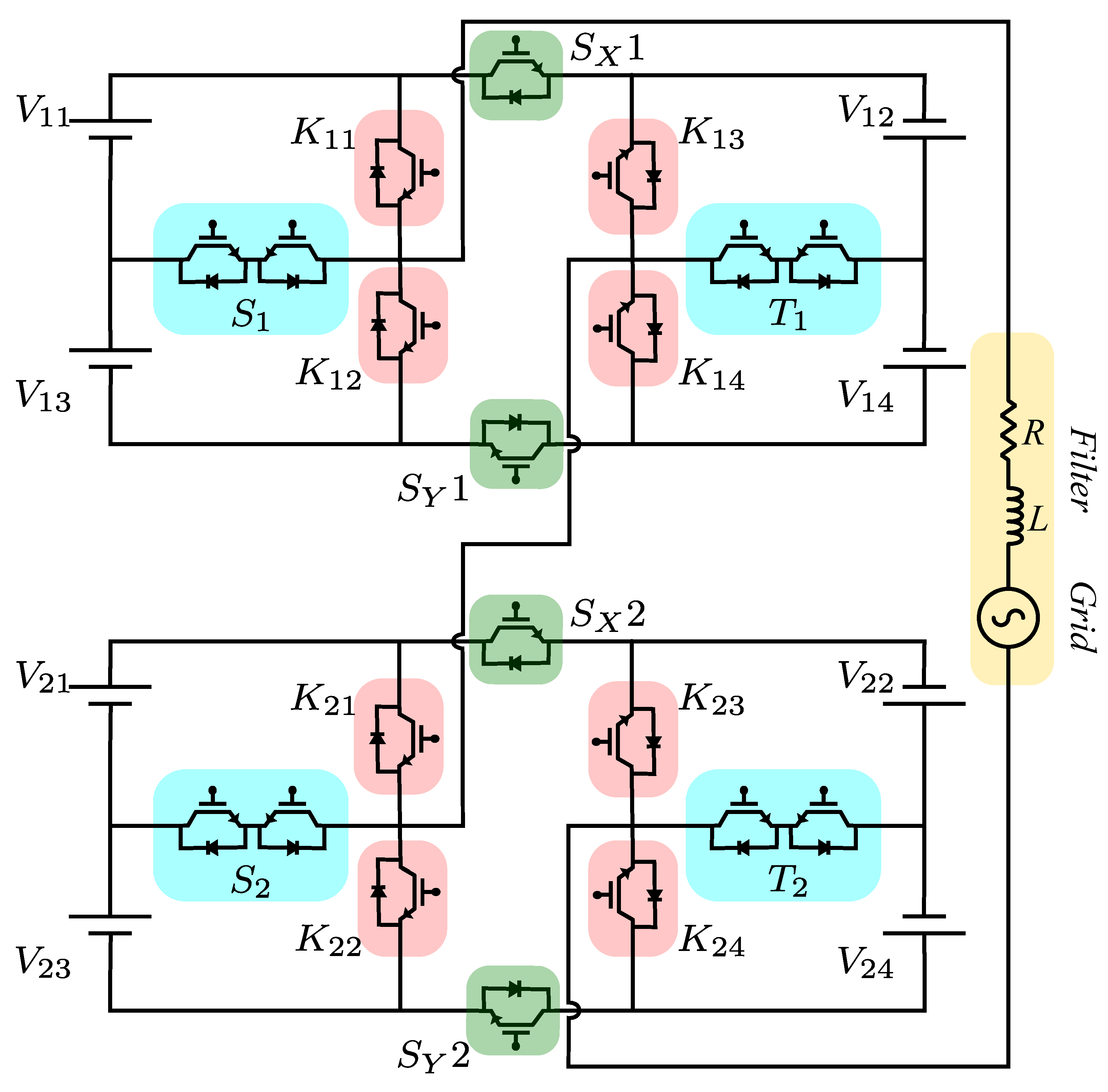
Figure 2.
Extrapolation of current using vector angle.
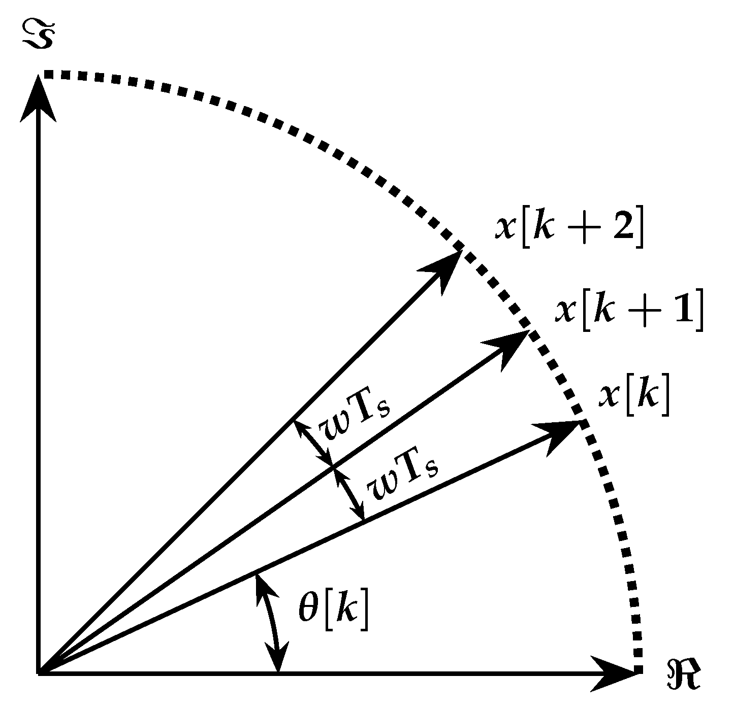
Figure 3.
State-Sector diagram for 289-level LMLI.
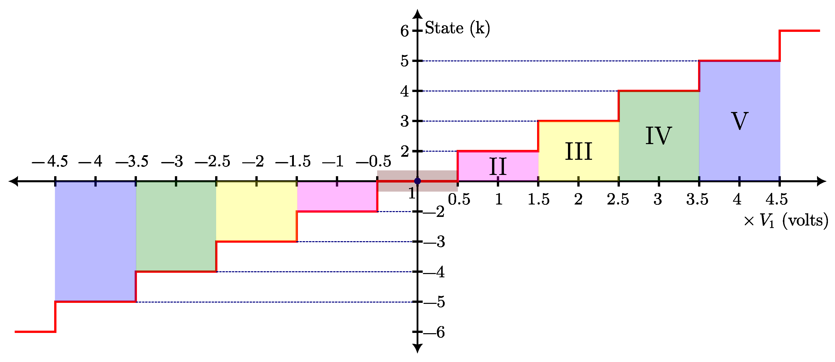
Figure 4.
Block diagram of Proposed DMPC of Three-Phase Grid Tied Inverter.

Figure 5.
Steady-state voltage of 289-level LMLI (a) L = 12 mH (b) L = 2 mH.

Figure 6.
Steady-state current of 289-level LMLI (a) L = 12 mH (b) L = 2 mH.
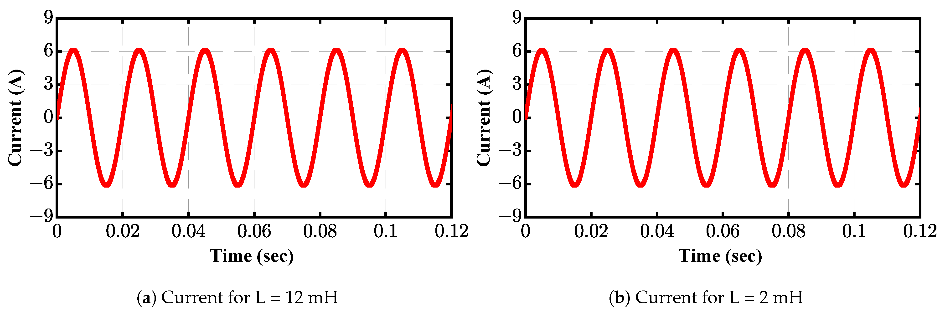
Figure 7.
Fourier analysis of voltage and current waveform @ L = 12 mH.

Figure 8.
Fourier analysis of voltage and current waveform @ L = 2 mH.
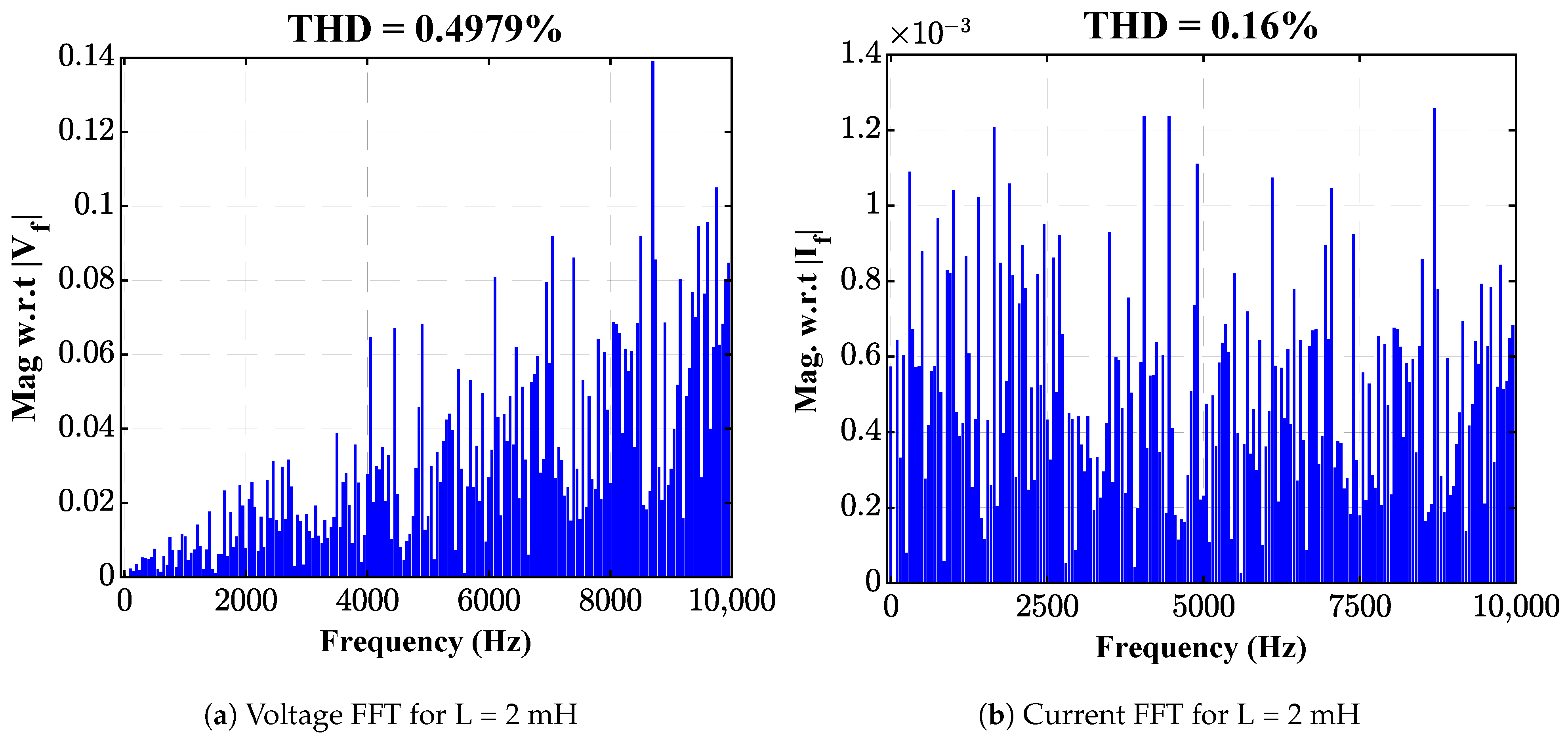
Figure 9.
Voltage of 289-level LMLI under step disturbance of current (a) L = 12 mH (b) L = 2 mH.

Figure 10.
Step change in current of 289-level LMLI (a) L = 12 mH (b) L = 2 mH.
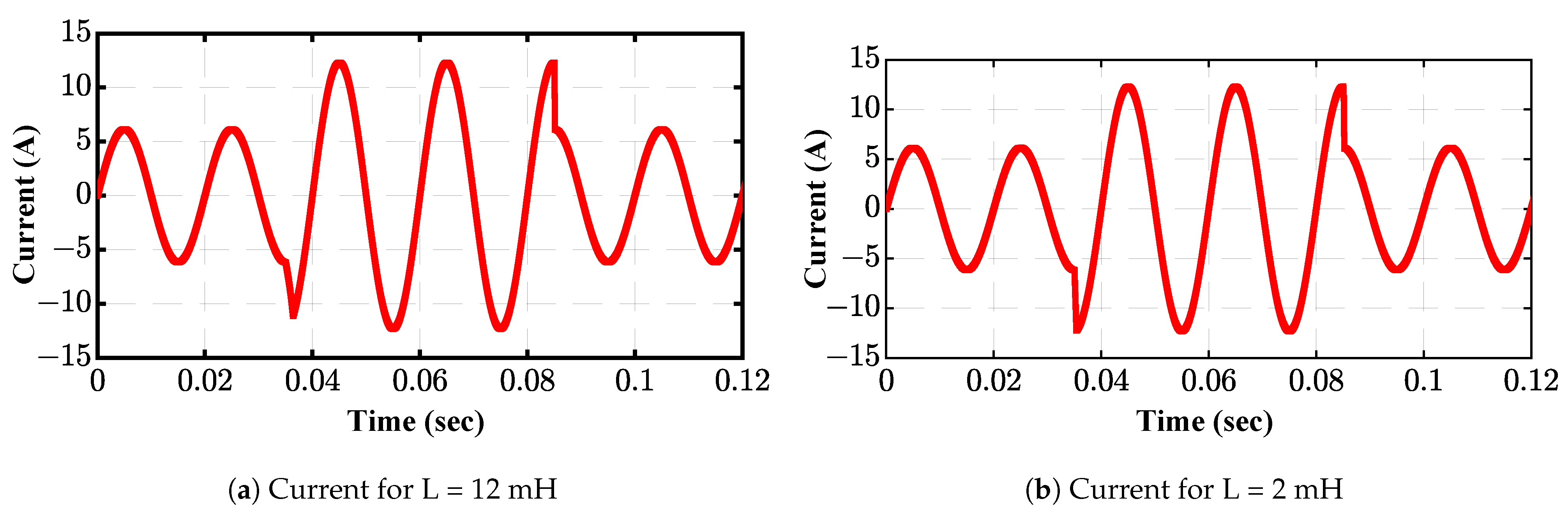
Figure 11.
Spotlight over step perturbation @ 35 ms with L = 12 mH.
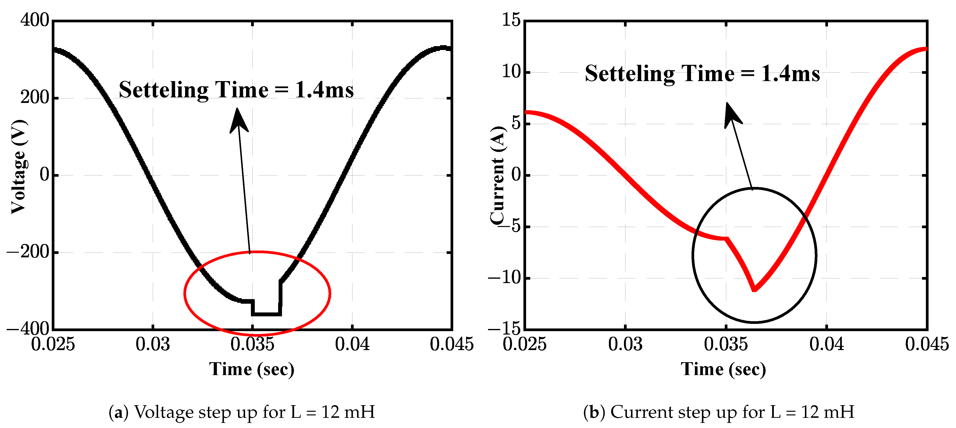
Figure 12.
Focused view of step down disturbance @ 85 ms with L = 12 mH.
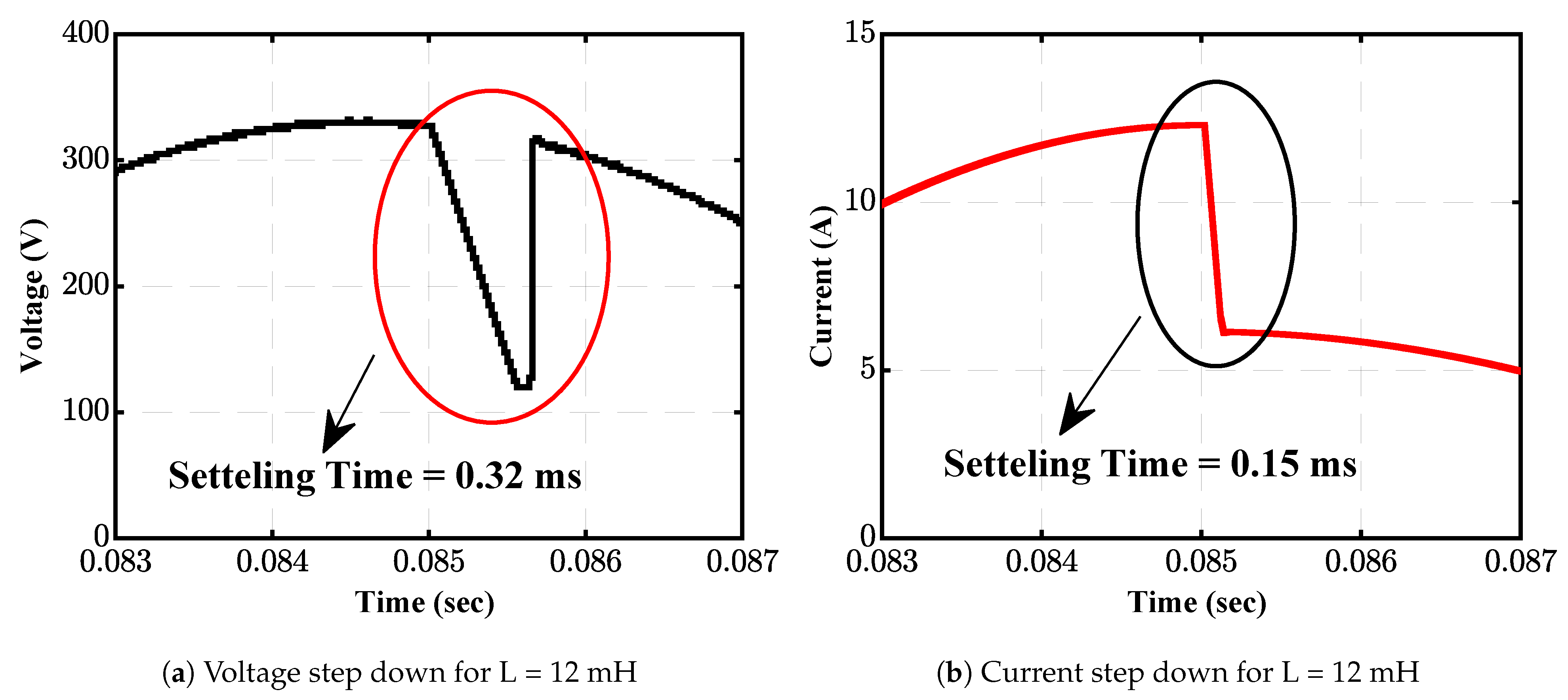
Figure 13.
Voltage of 289-level LMLI under parametric variation.
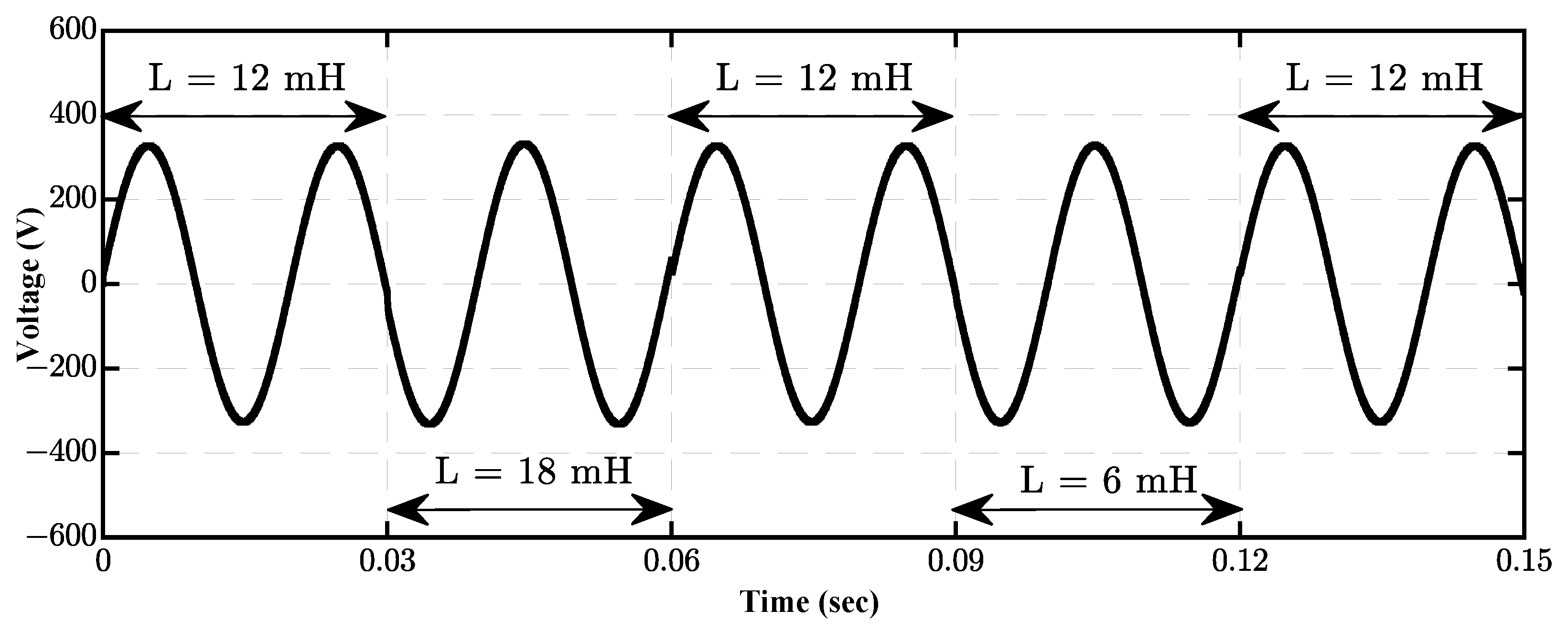
Figure 14.
Current of 289-level LMLI under parametric variation.
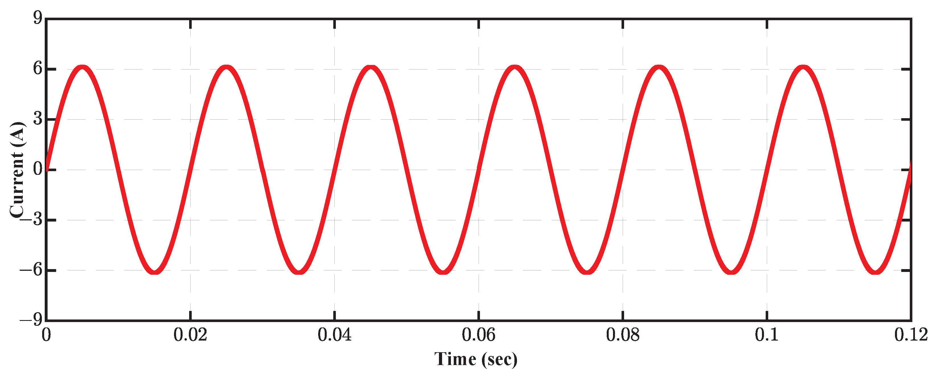
Figure 15.
High effect with traditional DMPC during step disturbance.

Table 1.
Switching States of 289-level Switch-ladder Structure.
| Switching States for 289-Level LMLI | |||||||||||||||||
|---|---|---|---|---|---|---|---|---|---|---|---|---|---|---|---|---|---|
| No. | |||||||||||||||||
| 1 | 1 | 0 | 1 | 0 | 0 | 0 | 1 | 0 | 1 | 0 | 1 | 0 | 0 | 0 | 1 | 0 | 0 |
| 2 | 0 | 0 | 0 | 1 | 1 | 0 | 0 | 1 | 1 | 0 | 1 | 0 | 0 | 0 | 1 | 0 | |
| 3 | 0 | 0 | 1 | 0 | 1 | 0 | 1 | 0 | 1 | 0 | 1 | 0 | 0 | 0 | 1 | 0 | |
| 4 | 0 | 1 | 0 | 0 | 0 | 1 | 0 | 1 | 1 | 0 | 1 | 0 | 0 | 0 | 1 | 0 | |
| 5 | 1 | 0 | 0 | 0 | 0 | 1 | 1 | 0 | 1 | 0 | 1 | 0 | 0 | 0 | 1 | 0 | |
| 6 | 1 | 0 | 0 | 1 | 0 | 0 | 0 | 1 | 1 | 0 | 1 | 0 | 0 | 0 | 1 | 0 | |
| 7 | 0 | 1 | 1 | 0 | 0 | 0 | 1 | 0 | 1 | 0 | 1 | 0 | 0 | 0 | 1 | 0 | |
| 8 | 0 | 1 | 1 | 0 | 0 | 0 | 0 | 1 | 1 | 0 | 1 | 0 | 0 | 0 | 1 | 0 | |
| 9 | 1 | 0 | 0 | 1 | 0 | 0 | 1 | 0 | 1 | 0 | 1 | 0 | 0 | 0 | 1 | 0 | |
| 10 | 0 | 0 | 0 | 0 | 1 | 1 | 0 | 1 | 1 | 0 | 1 | 0 | 0 | 0 | 1 | 0 | |
| 11 | 0 | 0 | 0 | 0 | 1 | 1 | 1 | 0 | 1 | 0 | 1 | 0 | 0 | 0 | 1 | 0 | |
| 12 | 1 | 0 | 0 | 0 | 0 | 1 | 0 | 1 | 1 | 0 | 1 | 0 | 0 | 0 | 1 | 0 | |
| 13 | 0 | 1 | 0 | 0 | 0 | 1 | 1 | 0 | 1 | 0 | 1 | 0 | 0 | 0 | 1 | 0 | |
| 14 | 0 | 0 | 1 | 0 | 1 | 0 | 0 | 1 | 1 | 0 | 1 | 0 | 0 | 0 | 1 | 0 | |
| 15 | 0 | 0 | 0 | 1 | 1 | 0 | 1 | 0 | 1 | 0 | 1 | 0 | 0 | 0 | 1 | 0 | |
| 16 | 1 | 0 | 1 | 0 | 0 | 0 | 0 | 1 | 1 | 0 | 1 | 0 | 0 | 0 | 1 | 0 | |
| 17 | 0 | 1 | 0 | 1 | 0 | 0 | 1 | 0 | 1 | 0 | 1 | 0 | 0 | 0 | 1 | 0 | |
| ⋮ | ⋮ | ⋮ | ⋮ | ⋮ | ⋮ | ⋮ | ⋮ | ⋮ | ⋮ | ⋮ | ⋮ | ⋮ | ⋮ | ⋮ | ⋮ | ⋮ | ⋮ |
| 189 | 0 | 1 | 1 | 0 | 0 | 0 | 1 | 0 | 0 | 0 | 0 | 1 | 1 | 0 | 0 | 1 | |
| ⋮ | ⋮ | ⋮ | ⋮ | ⋮ | ⋮ | ⋮ | ⋮ | ⋮ | ⋮ | ⋮ | ⋮ | ⋮ | ⋮ | ⋮ | ⋮ | ⋮ | ⋮ |
| 289 | 0 | 1 | 0 | 1 | 0 | 0 | 1 | 0 | 0 | 1 | 0 | 1 | 0 | 0 | 1 | 0 | |
Disclaimer/Publisher’s Note: The statements, opinions and data contained in all publications are solely those of the individual author(s) and contributor(s) and not of MDPI and/or the editor(s). MDPI and/or the editor(s) disclaim responsibility for any injury to people or property resulting from any ideas, methods, instructions or products referred to in the content. |
© 2023 by the authors. Licensee MDPI, Basel, Switzerland. This article is an open access article distributed under the terms and conditions of the Creative Commons Attribution (CC BY) license (https://creativecommons.org/licenses/by/4.0/).
Share and Cite
MDPI and ACS Style
Baig, M.A.; Kashif, S.A.R.; Khan, I.A.; Abbas, G. Quick Search Algorithm-Based Direct Model Predictive Control of Grid-Connected 289-Level Multilevel Inverter. Electronics 2023, 12, 3312. https://doi.org/10.3390/electronics12153312
AMA Style
Baig MA, Kashif SAR, Khan IA, Abbas G. Quick Search Algorithm-Based Direct Model Predictive Control of Grid-Connected 289-Level Multilevel Inverter. Electronics. 2023; 12(15):3312. https://doi.org/10.3390/electronics12153312
Chicago/Turabian StyleBaig, Muhammad Anas, Syed Abdul Rahman Kashif, Irfan Ahmad Khan, and Ghulam Abbas. 2023. "Quick Search Algorithm-Based Direct Model Predictive Control of Grid-Connected 289-Level Multilevel Inverter" Electronics 12, no. 15: 3312. https://doi.org/10.3390/electronics12153312
Note that from the first issue of 2016, this journal uses article numbers instead of page numbers. See further details here.