Abstract
Infrared and visible images of the same scene are fused to produce a fused image with richer information. However, most current image-fusion algorithms suffer from insufficient edge information retention, weak feature representation, and poor contrast, halos, and artifacts, and can only be applied to a single scene. To address these issues, we propose a novel infrared and visual image fusion algorithm based on a bilateral–least-squares hybrid filter (DBLSF) with the least-squares and bilateral filter hybrid model (BLF-LS). The proposed algorithm utilizes the residual network ResNet50 and the adaptive fusion strategy of the structure tensor to fuse the base and detail layers of the filter decomposition, respectively. Experiments on 32 sets of images from the TNO image-fusion dataset show that, although our fusion algorithm sacrifices overall time efficiency, the Combination 1 approach can better preserve image edge information and image integrity; reduce the loss of source image features; suppress artifacts and halos; and compare favorably with other algorithms in terms of structural similarity, feature similarity, multiscale structural similarity, root mean square error, peak signal-to-noise ratio, and correlation coefficient by at least 2.71%, 1.86%, 0.09%, 0.46%, 0.24%, and 0.07%; and the proposed Combination 2 can effectively improve the contrast and edge features of the fused image and enrich the image detail information, with an average improvement of 37.42%, 26.40%, and 26.60% in the three metrics of average gradient, edge intensity, and spatial frequency compared with other algorithms.
1. Introduction
The aim of infrared and visible image-fusion technology is to extract and integrate features from images captured by different sensors using specific algorithms, thereby generating a complementary image that contains both rich detailed features of the visible image and target information of the infrared image [1,2]. This technology has a wide-ranging impact on economic development, involving applications in fields such as national defense, military [3], intelligent transportation [4], and power grid operation [5,6]. These applications require advanced electronic components and control systems, such as high-performance sensors, image processors, and communication modules, which jointly promote technological progress and economic development.
Currently, among the numerous infrared and visible image fusion algorithms, the widely adopted approach is the image-fusion method based on multiscale transformation [7,8]. However, this method does not consider spatial inconsistencies well, which can lead to distortions and artifacts near the edges [9]. Moreover, its transformation and inverse transformation processes are time-consuming and complex, requiring a large amount of memory space and computational resources [10,11]. To overcome these problems, image fusion is performed using an edge-preserving smoothing filter [12], which can effectively avoid artifacts and spatial inconsistencies generated by multiscale transformations by decomposing the image into base and detail layers through filtering [13].
Ch et al. [14] proposed an image-fusion algorithm based on high-order discrete wavelet components and guided filters, which can effectively smooth and enhance spatial information, but halos still exist near the edges. Singh et al. [15] proposed an image-fusion method based on a discrete wavelet transform and a bilateral filter to better preserve the edges of the image, but it reduces the contrast of the infrared image in the fused image. Li et al. [16] proposed an image-fusion algorithm based on a fast approximate bilateral filter and local energy features, in which the algorithm utilizes a fast approximate bilateral filter to decompose the source image five times, obtaining a base layer and several detail layer images. However, the algorithm preserves edge features more efficiently at the expense of time and reduces halos.
As the development of deep learning has progressed in fields such as object detection and image restoration, various deep-learning-based algorithms have also been applied to image fusion. These algorithms can extract significant features from source images, such as convolutional neural networks (CNNs) [17] and generative adversarial networks (GANs) [18]. Liu et al. [19] proposed a CNN-based fusion algorithm, that works with the result of the last layer as image features, and the network structure is too simple, resulting in the loss of useful information. To solve the issue of information loss caused by the increase of convolutional networks, residual networks (ResNets) [20] and dense convolutional networks (DenseNets) [21] make full use of and process deep features to ensure that more useful information can be retained during feature extraction. However, the image-fusion algorithms of these methods require the manual design of fusion layers and do not achieve true automatic image fusion. To alleviate the complexity of engineering design, recently proposed approaches utilize end-to-end network models for image fusion, such as Fusion2Fusion [22], ZMFF [23], and SwinFuse [24]. However, these methods cannot fully utilize the complex characteristics and face challenges in effectively preserving the original details.
In summary, although the smoothing filtering algorithms can provide edge protection, they do not sufficiently enable the extraction of image features. Additionally, if only the deep information of the image is extracted using the convolutional network during the fusion process [25], it can effectively improve the similarity of the fused image. However, this ignores important edge information, leading to drawbacks such as insufficient extraction of edges or textures in the fused image. To better extract the feature information of source images, enhance image contrast, and effectively preserve image edges, this paper is inspired by the mixed filtering proposed by Liu et al., and proposes an infrared and visible image fusion algorithm based on second-order bilateral–least-squares mixed filtering [26]. In this algorithm, a quadratic bilateral–least-squares mixed filtering model is used to decompose the source images into detail layer 1. The amplified detail layer 1 and the source image are then fused using a second decomposition to obtain detail layer 2 with sharper boundaries and more edge information, as well as a base layer. Multiple feature layers are extracted using ResNet50 and a high-quality saliency map is generated for weighted fusion with the base layer. Additionally, an adaptive weighted method based on the structure tensor is used to fuse the two detail layers obtained from the two decompositions. Finally, different combinations of the fused base layer, detail layer 1, and detail layer 2 are used to obtain the desired fusion image for multiple scenes. The contributions of this work are summarized as follows.
- (1)
- This work proposes an infrared and visible image fusion algorithm based on a dual bilateral–least-squares hybrid filter. The hybrid filter achieves spatial consistency, edge preservation, and texture smoothing to solve halo artifacts around the edges and reduce noise in the fusion of infrared and visible images. Meanwhile, this paper provides two different layer combination methods, which can better adapt to the engineering application requirements.
- (2)
- The proposed image-fusion method applies a two-stage decomposition method with a bilateral–least-squares hybrid filter to obtain enhanced edge details from the source image. The adaptive weighting strategy based on the structure tensor is more effective in preserving the contour features present in the detail layer.
- (3)
- The proposed method utilizes the residual network’s strong feature preservation and extraction capabilities to fuse the base layer, which contains many pieces of fundamental information in the image. This approach effectively retains essential information in the base layer and enhances the image’s feature similarity.
- (4)
- The effectiveness and adaptability of a novel dual bilateral–least-squares hybrid filter (DBLSF)-based method for fusing infrared and visible images have been validated through experiments on 32 TNO datasets. The results indicate that Combination 1 can better maintain the image edge information and integrity while reducing the loss of important information features from the source images. On the other hand, Combination 2 is more proficient in enhancing contrast and edge features.
The remaining sections of the paper are presented as follows. Section 2 provides a brief overview of the fundamental principles behind the bilateral filter and least-squares filter. Section 3 outlines the proposed image-fusion method. Section 4 describes the experimental results and analysis. Lastly, Section 5 presents the conclusions.
2. Principle of the Bilateral–Least-Squares Filtering Algorithm
The bilateral–least-squares filtering algorithm is a hybrid filtering method that combines the ideas of bilateral filtering and the least-squares method, considering both the spatial and pixel value domain correlation. It effectively enhances image contrast while preserving edge information. Specifically, bilateral filtering is a non-linear filtering method that preserves edge information while removing noise, while the least-squares method is a mathematical optimization technique that uses the best-fitting of the curve to minimize the error between predicted and true values.
2.1. Bilateral Filter
A key issue in image smoothing filtering is effectively preserving edge information, as it greatly impacts the quality of the resulting fused image. Bilateral filters use functions composed of spatial and color information to effectively smooth images while preserving edge information [27]. For a given input image, with s as the central point and t as the image of any point in s’s neighborhood N(s), the output image after being processed by a bilateral filter is denoted as , as shown in (1).
where and are spatial and Gaussian kernel functions, respectively. represents the spatial proximity factor and grayscale similarity factor. represents the spatial distance between point t in neighborhood N(s) and other points, while represents the difference in the gray value.
When it comes to image smoothing and edge preservation, bilateral filtering may cause gradient reversal and halo effects, and it is difficult to effectively remove strong speckle noise. In contrast, weighted least-squares filtering only performs smoothing filtering in flat areas, achieving the effect of noise removal and edge preservation.
2.2. Least-Squares Filter
The least-squares method is a mathematical optimization technique that seeks the best-fitting curve to minimize the error between predicted and true values. The weighted least-squares filter is a filtering method based on the least-squares method, which can efficiently extract background information and texture details from different spatial scales of the source image [28]. In the weighted least-squares filter, the weight values in the weight matrix depend on the local characteristics of the signal, such as the slope, curvature, and second-order derivative of the signal. By adjusting the weight matrix, a balance between noise suppression and edge protection can be achieved during the filtering process, and the quality of image filtering is further improved. The image of a center point s can be obtained by minimizing the following objective function:
where the first minimizes the difference between and ; the second term is smoothed by minimizing the partial derivative of ; is a regular factor; and and are smoothing weights.
The and value can be derived by the following formulas:
where is the logarithmic luminance channel of the input image ; that is, = log(). The parameter determines the sensitivity of the gradient of and (usually 0.0001) is a small constant to prevent division by zero in constant regions of image .
Taking the derivative of the objective function (2) and setting it to zero yields the large sparse linear system represented by (4):
In (4), , where and are diagonal matrices containing and , respectively. and are forward difference operators, while and are backward difference operators. Therefore, is a nonhomogeneous Laplacian matrix with five points.
The linear system of equations in (4) can be utilized to derive a vector that minimizes (2). The solution to this quadratic optimization problem, subject to linear constraints, can be expressed as follows:
However, computing the nonhomogeneous Laplacian matrix in (4) incurs a high computational cost and causes (5) to be solved in the image domain, resulting in a very large inverse matrix. Therefore, setting = = 1 in (2) can turn it into an unweighted equation, as shown in (6).
Since (6) is the unweighted least-squares method and is the Laplacian matrix in (5), the smallest unique vector solution can be obtained in the Fourier domain. Then, the output image can be obtained by the following formula:
where and are the fast Fourier transform (FFT) and inverse fast Fourier transform (IFFT) operators, respectively. and are complex conjugates. represents that the fast Fourier transform of the δ function is always 1. Addition, multiplication, and division operations are all pointwise operations.
The advantage of unweighted least-squares filtering is the fast and efficient computation of the vector solution using FFT and IFFT operators. However, it lacks an edge-preserving smoothing operator, leading to halo artifacts in the filtered image.
2.3. Bilateral–Least-Squares Filtering Algorithm
This paper proposes a new method based on the approach presented in [24], called bilateral least-squares filtering (BLF-LS), for smooth images. This method first uses bilateral filtering to smooth the image gradient and then embeds the smoothed image gradient into a least-squares framework, effectively smoothing the image while better preserving its edges. Specifically, the smoothing framework is implemented as follows:
where, when is sufficiently large, the gradient of the output , i.e., , will approach , .
where , represents smoothing of the gradient of the input image in the and axes directions using bilateral filtering, and represents smoothing of the input image using BLF-LS filtering.
Combining bilateral filtering and least-squares filtering can achieve complementary effects, because bilateral filtering can preserve the structure of image information well but may lose a lot of shadow distribution, while least-squares filtering can preserve the shadow distribution of reference information well but may lose the edge structure and detail information of image information. Therefore, combining the two filtering methods can better preserve the edge structure and detail information of the image while preserving the image structure information and shadow distribution, thus achieving a better image filtering effect.
3. Dual Bilateral–Least-Squares Hybrid Filtering Model
The bilateral–least-squares hybrid filtering model is a filtering algorithm used for image denoising. This algorithm combines the advantages of bilateral filtering and least-squares filtering, and can effectively remove noise from images while preserving the details and edge information. In this way, the dual bilateral–least-squares hybrid filtering (DBLSF) model can simultaneously meet the requirements of image smoothing and denoising and can be applied to many image processing tasks, such as digital image processing, computer vision, and robot vision.
3.1. Image-Fusion Model
Given the input visible image and infrared image , the filtering models in this paper are employed to decompose the visible and infrared input images into the base layer and detail layer , . The fusion weighting strategy in the proposed model is chosen based on the different contrast and detail features of the decomposed base layer and detail layer. The base layer is deeply extracted with a residual network (ResNet50) to obtain base layer features, and the corresponding weight map is calculated by local L1-norm and average operation. The detail layer adopts an adaptive weighting strategy based on structural tensor for fusion. The fusion algorithm presented in this study follows a flowchart, as depicted in Figure 1, which involves combining the fused base layer and detail layer to obtain the fused image F. Two combinations are defined based on the combination of the detail layer and the base layer, namely Combination 1 (C1), which includes only detail layer 1 and the base layer, and Combination 2 (C2), which includes detail layer 1, detail layer 2, and the base layer.
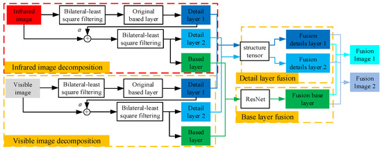
Figure 1.
Flowchart of infrared and visible image fusion algorithm based on DBLSF.
The base layer is obtained by filtering the input image with BLF-LS. The detail layer is obtained by subtracting the basic layer from the input image . The calculation formula is shown below.
3.2. Fusion Rules
The basic layer contains low-frequency content, including a large amount of basic information about the image, and represents the overall appearance of the image in smooth areas. Therefore, effectively extracting the features of the basic layer and preserving a large amount of information from the source image can improve the similarity between the fusion image and the source image. In this paper, DBLSF is used to decompose the source image into a basic layer and a detail layer, as shown in Figure 2.
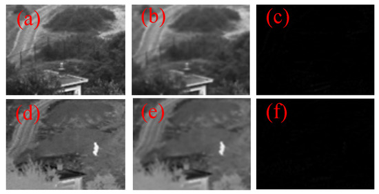
Figure 2.
Base layers and detail layers obtained by BLF-LS decomposition of the source image. (a) Visible image; (b) base layer of visible image; (c) detail layer of visible image; (d) infrared image; (e) base layer of infrared image; (f) detail layer of infrared image.
To obtain more detailed information, this paper enhances the source image and obtains the base layer through (12).
where is an adjustable parameter, which is used to amplify the detail layer and added to the source image to obtain the enhanced image.
Finally, the base layer of the source image is enhanced using (13):
In (12), when is 0, it represents the original basic layer. Setting different values of to enhance the contrast of the base layer is necessary to ensure its correlation and visual perception with the original basic layer. The enhanced basic layer was compared with the original basic layer through objective evaluation metrics such as average gradient (AG), structural similarity (SSIM), visual information fidelity (VIF), and correlation coefficient (CC). The decomposed images of infrared and visible obtained are shown in Figure 3 and Figure 4, respectively, and corresponding objective evaluation results with varying parameters are shown in Table 1.
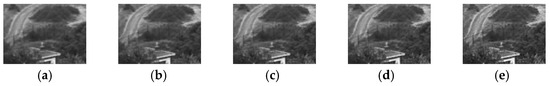
Figure 3.
obtained by decomposition of different . (a) = 0.5; (b) = 1.0; (c) = 1.5; (d) = 2.0; (e) = 3.0.
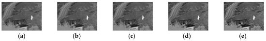
Figure 4.
obtained by decomposition of different . (a) = 0.5; (b) = 1.0; (c) = 1.5; (d) = 2.0; (e) = 3.0.

Table 1.
The image of the decomposition obtained by changing the variable with the corresponding objective evaluation.
Based on the results in Table 1, it was found that, when > 1, the smoothed basic layer showed a significant increase in AG, but noise severely affected the visual perception, and the correlation coefficient between the original basic layer and the enhanced basic layer was reduced. Therefore, a value of = 1 was chosen, which provided a visually pleasing and highly correlated basic layer, and effectively improved the overall brightness and contrast of the image.
3.2.1. ResNet50-Based Fusion
The enhanced base layer B contains important image details, as well as the primary contrast and brightness information. To better preserve the background features of the source image and improve the similarity between the fused image and the source image, ResNet50 trained on ImageNet was used to obtain deep features. Then, a multi-layer fusion strategy was employed to obtain a weight map. Finally, the weight map and the base layer were fused. The process of base layer fusion is illustrated in Figure 5.
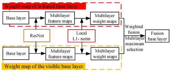
Figure 5.
Flowchart of base layers’ fusion.
The fusion strategy using ResNet50 for extracting deep features is described in detail below. ResNet50 consists of 5 convolutional blocks and the output feature maps can be represented as , .
where represents the process of extracting the feature map by the i-th convolutional block in ResNet50. The more convolutional blocks the input image passes through, the more abstract image features are extracted, generating deeper and higher-semantic feature maps. Therefore, in this study, we chose the deep feature maps outputted from the i = 3, 4, 5 convolutional blocks. Among them, the feature maps and with i = 3, 4 are saved during the extraction of deep feature maps with i = 5, rather than using different networks for extraction (as in Li et al. [19]), thus saving time.
The workflow diagram for generating deep feature maps using ResNet50 is shown in Figure 6 and the corresponding time consumption is listed in Table 2, with the optimal values highlighted in bold. The initial weights for calculating the feature map using local L1-norm and averaging are computed using the following formula:
where represents the L1-norm, (p, q) represents the coordinates within the region, and t = 2 is used in this paper.
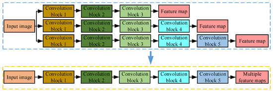
Figure 6.
Flowchart of generating depth feature maps using ResNet50.
Table 2.
Extraction of feature maps using ResNet50 network time consumed.
Due to the use of residual networks in extracting deep features, the number of channels M in the feature map varies with the number of convolutional blocks i, with the following relationship: . Therefore, it is necessary to perform bicubic interpolation on the initial weight w to adjust it to the size of the input base layer and then calculate the final weight map. The calculation formula is as follows:
The fusion of the input base layer with the weight map , ( and ) obtained is calculated as shown in (18):
Finally, the maximum modulus method is used to fuse the base layer. The maximum value of the base layer is calculated by (19).
3.2.2. Structure Tensor-Based Fusion
The gradient values of an image are closely related to its visual effects and, the larger the gradient values of the image, the more obvious its fine texture and edge features [29]. Using a structure tensor-based adaptive weighting strategy [30,31] can better preserve the spatial information and detail layer features of the image. As shown in Figure 2, the decomposed detail layer contains high-frequency content, mainly including edge, contour, and sharp detail information. To construct the structure tensor gradient , of the input detail layer , the partial derivatives and along the x and y axis are computed. The specific calculation formulas are as follows:
The matrix and are both symmetric positive definite matrices, so they can be decomposed as:
where and are two non-negative eigenvalues of matrix , and their corresponding eigenvectors are and , respectively.
Assuming that the larger eigenvalue is and the smaller one is , a larger value indicates stronger edge intensity at that pixel in the image. Meanwhile, in terms of the Frobenius norm, the fused image should preserve the properties of the original images and its should be closest to , that is, , where is the following matrix:
According to the eigenvector corresponding to the larger eigenvalue , it represents the gradient direction of the pixel point, which has the most obvious gray level changes and stronger edge intensity, indicating richer spatial information. Therefore, the weight matrices and for the detail layers of the visible and infrared images can be, respectively, calculated using the proportion of the larger eigenvalue and .
Finally, the fused detail layer can be calculated using the weighted method, which is expressed as
where is the fused detail layer, and are the detail layers of the visible and infrared images, respectively, and .* represents the dot product, which means multiplying the numerical values at the same coordinate positions of two image matrices the same size.
4. Experiment Results and Analysis
The experimental simulation platform utilized in this study consists of a notebook computer with an Intel(R) Core(TM) i7-8750H processor operating at 2.20 GHz and with 8.00 GB of RAM. The programming environment employed is MATLAB R2021b and the operating system of the computer is 64-bit Windows 10.
4.1. Algorithm Comparison and Parameter Settings
The effectiveness of the proposed fusion algorithm was evaluated through experiments conducted on infrared and visible images from the TNO image-fusion dataset [32]. To compare the performance of the proposed method, Combination 1 (C1) and Combination 2 (C2) with 13 existing infrared and visible image fusion algorithms, including MDLatLRR [33], MGF [34], and multiscale transform enhancement (MST-TE) [35], were tested. The experimental parameters for these 14 algorithms were set based on their original papers. In the proposed algorithm of this article, small values of and may lead to gradient reversal, while larger values of and enhance the smoothing ability, but may generate halos. In this article, we set = 2, = 0.04, = 2, = 3 = 0.12 to preserve the regions with large intensity differences and to better retain the edge information of the images, thus improving the smoothing ability of the algorithm.
4.2. Fusion Results
As there are too many fusion image results of the infrared and visible light, we cannot display all of them. Therefore, this paper selects three sets of the TNO image-fusion dataset (the 14th image of Nato_camp_sequence, soldier-behind_smoke_3, and Kaptein_1123) to show the output results. Figure 7 illustrates the three sets of infrared and visible images, and Figure 8, Figure 9 and Figure 10 demonstrate the resulting output for each set. Red rectangular boxes are used to help distinguish the quality of the fused images.
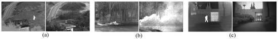
Figure 7.
The three sets of infrared and visible images. (a) The 14th image of Nato_camp_sequence; (b) soldier-behind_smoke_3; (c) Kaptein_1123.
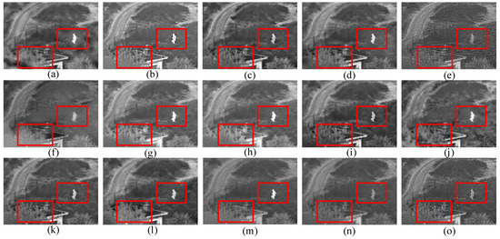
Figure 8.
The first set of experiments results. (a) NSCT; (b) MDLatLRR; (c) MGF; (d) MST-SR; (e) FPDE; (f) GTF; (g) CBF; (h) IFEVIP; (i) Hybrid-MSD; (j) NSCT-SR; (k) TIF; (l) CNN; (m) MST-TE; (n) proposed method (C1); (o) proposed method (C2).
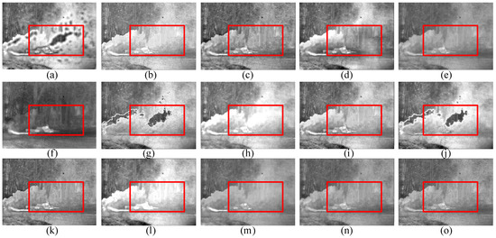
Figure 9.
The second set of experiments results. (a) NSCT; (b) MDLatLRR; (c) MGF; (d) MST-SR; (e) FPDE; (f) GTF; (g) CBF; (h) IFEVIP; (i) Hybrid-MSD; (j) NSCT-SR; (k) TIF; (l) CNN; (m) MST-TE; (n) proposed method (C1); (o) proposed method (C2).
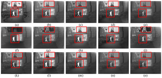
Figure 10.
The third set of experiments results. (a) NSCT; (b) MDLatLRR; (c) MGF; (d) MST-SR; (e) FPDE; (f) GTF; (g) CBF; (h) IFEVIP; (i) Hybrid-MSD; (j) NSCT-SR; (k) TIF; (l) CNN; (m) MST-TE; (n) proposed method (C1); (o) proposed method (C2).
4.3. Subjective Evaluation
For the first set of experiments depicted in Figure 8, all 14 methods demonstrated the ability to effectively combine the details of the infrared images with the context information of the visible images. However, images (a) and (e) contain more noise, resulting in a visually blurry image and relatively poor visual effects. Image (b) has overall brightness that is too high, losing important information in the visible image and containing more noise. In the case of images (c), (f), and (i), the comparison between the objects and the background is relatively low. In particular, image (f) shows a lack of texture near the figure, which hinders the observation of the fence. Image (d) has an obvious block effect and the detail part of image (g) has good performance, but the wavelet transform produces a residual shadow, and image (l) has partial distortion due to the convolution process. In images (h) and (j), the significant features of grass, trees, and fences are not obvious, and the background information is severely lost. When compared to images (k) and (m), image (n) effectively retains the grass information from both the infrared and visible images and accurately represents the source image’s characteristic features. Meanwhile, image (o) enhances the details of the fence and grass, resulting in higher overall contrast and sharper edges.
In the second set of experimental results, Figure 9, images (a), (g), and (j) contain a large number of artifacts, which make the task target unclear and not conducive to human recognition. When images (b) and (l) retain relatively complex detail, they fail to highlight distinctive traits of the image, such as the loss of detail in the tree above the person on the right side of the image. Images (c), (d), and (k) do not produce halos but lack some details. Images (e), (f), and (m) contain more noise and severely lose their texture features in dense smoke areas. Image (h) lacks visible image texture information due to the minimal incorporation of visible image features. In contrast, image (i) is better at identifying the target but shows image discontinuity. The results obtained using Combination 1 of the proposed fusion algorithm, represented by image (n), highlight the target clearly, contain fewer artifacts, and do not exhibit double images or visual blurs. Meanwhile, image (o) successfully retains the overall message of the original image and the salient features of the objects are distinctly visible.
The results of the third set of experiments in Figure 10 show that images (a), (g), and (j) contain a significant amount of artifacts and noise in the background, resulting in poor visual perception. The overall brightness of images (d) and (e) is poor, and the contrast is not high. In image (l), the target person stands out prominently but the grass details are lost. Image (c) and image (i) have artifacts around the target person. Image (f) has low contrast and unclear edge information. Images (b) and (k) have circular artifacts around the edge of the target, resulting in lost edge details and poor visual perception. The details in Figure (m) and Figure (h) are not prominent enough. Relatively speaking, image (n) has less noise and effectively integrates valuable information from both infrared and visible images. On the other hand, image (o) presents sharper edge information, finer details, and higher contrast, indicating a better expression of these image features.
4.4. Objective Evaluation
The subjective evaluation of image quality is predicated on the subjective perception of the observer, which may be affected by differences in individual visual sensitivity and may lead to biased conclusions. Therefore, this paper combined quantitative indicators to comprehensively evaluate the quality of fusion images, whereas, as we all know, a single evaluation index cannot reflect the quality of the fused image well in quantitative evaluation. To evaluate the fusion performance of various fusion technologies more objectively, this paper selects nine commonly used fusion evaluation indicators, namely peak signal-to-noise ratio (PSNR), structural similarity (SSIM), feature similarity (FSIM), multiscale structural similarity (MS_SSIM), correlation coefficient (CC), root mean square error (RMSE), average gradient (AG), edge intensity (EI), and spatial frequency (SF). Among them, the first six indicators are used to evaluate the fusion quality of algorithm Combination 1 in this paper and the last three indicators are used to evaluate the fusion quality of algorithm Combination 2, mainly to reflect the contrast, clarity, and edge preservation of the fused image. With the exception of the RMSE index, the fusion performance improves with higher values of the other eight indicators. The stacked bar chart used for evaluating the fusion effect of three sets of images is shown in Figure 11, and Table 3 presents the objective evaluation results for 32 sets of image fusion using both infrared and visible light. The evaluation metric’s optimal value is indicated in bold within the table.
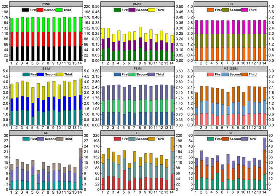
Figure 11.
Stacked histogram of the selected three sets of image-fusion effect evaluation.
Table 3.
Objective evaluation of 32 sets of infrared and visible image fusion.
The evaluation presented in Figure 11 demonstrates that the algorithm proposed in this paper outperforms Combination 1 and other algorithms in terms of RMSE and SSIM, indicating a reduction in image noise and better preservation of structural similarity. However, the low brightness of the third set of visible images makes it difficult to evaluate FSIM and MS_SSIM. Additionally, the feature similarity between Combination 1’s low brightness image and the source image is limited. The evaluation of AG, EI, and SF in the last row suggests that Combination 2 achieves optimal edge detail and contrast across various environments.
In Table 3, it can be seen that the algorithm proposed in this paper effectively preserves a large amount of information from the source image and improves the similarity with the source image by utilizing ResNet50 to fuse the base layers. Additionally, by adopting an adaptive weighting strategy based on the structural tensor model to process the multi-layer detail layers of the enhanced image after secondary decomposition, the algorithm can effectively fuse the texture features of the image details, highlighting its advantage in overall brightness and edge information in Combination 2. The following is a detailed analysis of the two combined effects of the proposed algorithm: (1) Combination 1 of this paper’s algorithm does not perform well in the AG, EI, and SF metrics, but it is the best in six metrics, including SSIM, FSIM, MS_SSIM, RMSE, PSNR, and CC, improving by 2.71%, 1.86%, 0.09%, 0.46%, 0.24%, and 0.07% compared with the other algorithms, respectively. This indicates that the fusion image of Combination 1 contains more effective information, has higher similarity to the characteristics of the source image, and contains less artificial noise in the fusion image. (2) The fusion image of Combination 2 improved by 37.42%, 26.40%, and 26.60% in the AG, EI, and SF metrics, respectively. The experimental results show that the fusion image of Combination 2 significantly improved in terms of contrast, preserving image edges and textures. In summary, this paper’s algorithm provides two combination methods that can be used to meet different needs in the engineering application of infrared and visible light image fusion.
Finally, two combinations of the algorithms in this paper were compared with 13 other algorithms in terms of time efficiency and the results are shown in Table 4.
Table 4.
Comparison of time efficiency of 14 image-fusion algorithms.
Since the algorithm proposed in this paper combines four modules, bilateral filtering, the least-squares model, the ResNet50 network, and the structure tensor model, it can better preserve high-quality images and adapt to the requirements of both scenes. The proposed algorithm is definitely more time efficient than MDLatLRR, NSCT_SR, and CNN. It sacrifices more time and fuses higher-quality images than other algorithms with multiscale transform and simple filter decomposition.
5. Conclusions
To improve the quality of fusion images and meet the application requirements of different scenes, in this article, we propose a novel fusion algorithm for infrared and visible images based on DBLSF. This article achieves the following objectives:
- (1)
- The hybrid filter is utilized in this paper to address the issues of halo artifacts around edges and noise reduction in the fusion results of infrared and visible images by achieving spatial consistency, edge preservation, and texture smoothing.
- (2)
- The algorithm presented in this paper offers two distinct combinations (C1 and C2) of the base layer and the multi-layer detail layer. Through experiments conducted on 32 TNO datasets, the effectiveness of both combinations in meeting the requirements of engineering applications is demonstrated.
- (3)
- Compared with the 13 existing algorithms, it is verified that C1 provides significant advantages in terms of similarity with the features and structure of the source image, as well as removing noise. The six indexes of SSIM, FSIM, MS_SSIM, RMSE, PSNR, and CC are improved by 2.71%, 1.86%, 0.09%, 0.46%, 0.24%, and 0.07%, respectively. On the other hand, C2 has more pronounced effects in preserving edge information and improving contrast. The AG, EI, and SF indexes increase by 37.42%, 26.40%, and 26.60%, respectively.
In addition, the algorithm described in this paper can also be applied to other image-fusion tasks, such as medical images, multi-focus images, remote sensing images, and multiple exposure images. In future research, we will consider combining more efficient edge smoothing filters with lightweight deep-learning algorithms to further improve the quality and speed of fused images.
Author Contributions
Conceptualization, L.H.; Software, Z.H.; Validation, Z.H.; Formal analysis, Z.H.; Investigation, Z.H.; Data curation, Z.H. and F.T.; Writing—original draft, Z.H.; Visualization, Z.H.; Project administration, Q.L. and L.H.; Funding acquisition, Q.L. All authors have read and agreed to the published version of the manuscript.
Funding
The National Natural Science Foundation of China provided financial support for this research through Grant 61863002, the Natural Science Foundation of Guangxi Province (China) under Grant AA22068071.
Data Availability Statement
The data posted on 26 April 2014, which can be obtained on the official website of figshare, with the address of https://doi.org/10.6084/m9.figshare.1008029.v1.
Acknowledgments
The authors would like to thank all anonymous reviewers for their helpful comments and suggestions.
Conflicts of Interest
The authors declare that they have no known competing financial interests or personal relationships that could have appeared to influence the work reported in this study.
References
- Ma, W.; Wang, K.; Li, J.; Yang, S.; Li, J.; Song, L.; Li, Q. Infrared and Visible Image Fusion Technology and Application: A Review. Sensors 2023, 23, 599. [Google Scholar] [CrossRef]
- Singh, S.; Singh, H.; Bueno, G.; Deniz, O.; Singh, S.; Monga, H.; Hrisheekesha, P.H.; Pedraza, A. A Review of Image Fusion: Methods, Applications and Performance Metrics. Digit. Signal Process. 2023, 137, 104020. [Google Scholar] [CrossRef]
- Ma, J.; Tang, L.; Xu, M.; Zhang, H.; Xiao, G. STDFusionNet: An Infrared and Visible Image Fusion Network Based on Salient Target Detection. IEEE Trans. Instrum. Meas. 2021, 70, 5009513. [Google Scholar] [CrossRef]
- Lu, M.; Liu, H.; Yuan, X. Thermal fault diagnosis of electrical equipment in substations based on image fusion. Traitement Signal 2021, 38, 1095–1102. [Google Scholar] [CrossRef]
- Gao, M.; Wang, J.; Chen, Y.; Du, C.; Chen, C.; Zeng, Y. An Improved Multi-Exposure Image Fusion Method for Intelligent Transportation System. Electronics 2021, 10, 383. [Google Scholar] [CrossRef]
- Fu, L.; Sun, L.; Du, Y.; Meng, F. Fault diagnosis of radio frequency circuit using heterogeneous image fusion. Opt. Eng. 2023, 62, 034107. [Google Scholar] [CrossRef]
- Li, Y.; Yang, H.; Wang, J.; Zhang, C.; Liu, Z.; Chen, H. An Image Fusion Method Based on Special Residual Network and Efficient Channel Attention. Electronics 2022, 11, 3140. [Google Scholar] [CrossRef]
- Vs, V.; Valanarasu, J.M.J.; Oza, P.; Patel, V.M. Image fusion transformer. In Proceedings of the 2022 IEEE International Conference on Image Processing (ICIP), Bordeaux, France, 16–19 October 2022; pp. 3566–3570. [Google Scholar]
- Li, G.; Lin, Y.; Qu, X. An infrared and visible image fusion method based on multi-scale transformation and norm optimization. Inf. Fusion 2021, 71, 109–129. [Google Scholar] [CrossRef]
- Han, X.; Lv, T.; Song, X.; Nie, T.; Liang, H.; He, B.; Kuijper, A. An Adaptive Two-Scale Image Fusion of Visible and Infrared Images. IEEE Access 2019, 7, 56341–56352. [Google Scholar] [CrossRef]
- Yang, Y.; Zhang, W.; Huang, S.; Wan, W.; Liu, J.; Kong, X. Infrared and Visible Image Fusion Based on Dual-Kernel Side Window Filtering and S-Shaped Curve Transformation. IEEE Trans. Instrum. Meas. 2022, 71, 5001915. [Google Scholar] [CrossRef]
- Jagtap, N.; Thepade, S.D. Enhanced Image Fusion with Guided Filters. In Object Detection by Stereo Vision Images; Scrivener Publishing LLC: Beverly, MA, USA, 2022; pp. 99–110. [Google Scholar]
- Ma, J.; Ma, Y.; Li, C. Infrared and visible image fusion methods and applications: A survey. Inf. Fusion 2019, 45, 153–178. [Google Scholar] [CrossRef]
- Ch, M.M.I.; Riaz, M.M.; Iltaf, N.; Ghafoor, A.; Ali, S.S. A multifocus image fusion using highlevel DWT components and guided filter. Multimed. Tools Appl. 2020, 79, 12817–12828. [Google Scholar] [CrossRef]
- Singh, S.; Singh, H.; Gehlot, A.; Kaur, J. IR and visible image fusion using DWT and bilateral filter. Microsyst. Technol. 2022, 29, 457–467. [Google Scholar] [CrossRef]
- Li, Z.; Lei, W.; Li, X.; Liao, T.; Zhang, J. Infrared and Visible Image Fusion via Fast Approximate Bilateral Filter and Local Energy Characteristics. Sci. Program. 2021, 2021, 3500116. [Google Scholar] [CrossRef]
- Ghandour, C.; El-Shafai, W.; El-Rabaie, S. Medical image enhancement algorithms using deep learning-based convolutional neural network. J. Opt. 2023, 52, 1–11. [Google Scholar] [CrossRef]
- Li, J.; Huo, H.; Li, C.; Wang, R.; Feng, Q. AttentionFGAN: Infrared and Visible Image Fusion Using Attention-Based Generative Adversarial Networks. IEEE Trans. Multimed. 2021, 23, 1383–1396. [Google Scholar] [CrossRef]
- Liu, Y.; Chen, X.; Cheng, J.; Peng, H.; Wang, Z.F. Infrared and visible image fusion with convolutional neural networks. Int. J. Wavelets Multiresolut. Inf. Process. 2018, 16, 1850018. [Google Scholar] [CrossRef]
- Li, H.; Wang, X.J.; Durrani, T.S. Infrared and visible image fusion with ResNet and zero-phase component analysis. Infrared Phys. Technol. 2019, 102, 103039. [Google Scholar] [CrossRef]
- Ren, K.; Zhang, D.; Wan, M.; Miao, X.; Gu, G.; Chen, Q. An Infrared and Visible Image Fusion Method Based on Improved DenseNet and mRMR-ZCA. Infrared Phys. Technol. 2021, 115, 103707. [Google Scholar] [CrossRef]
- Lu, C.; Qin, H.D.; Deng, Z.C.; Zhu, Z.B. Fusion2Fusion: An Infrared–Visible Image Fusion Algorithm for Surface Water Environments. J. Mar. Sci. Eng. 2023, 11, 902. [Google Scholar] [CrossRef]
- Hu, X.; Jiang, J.; Liu, X.; Ma, J. ZMFF: Zero-shot multi-focus image fusion. Inf. Fusion 2023, 92, 127–138. [Google Scholar] [CrossRef]
- Wang, Z.; Chen, Y.; Shao, W.; Li, H.; Zhang, L. SwinFuse: A residual swin transformer fusion network for infrared and visible images. IEEE Trans. Instrum. Meas. 2022, 71, 5016412. [Google Scholar] [CrossRef]
- Shopovska, I.; Jovanov, L.; Philips, W. Deep visible and thermal image fusion for enhanced pedestrian visibility. Sensors 2019, 19, 3727. [Google Scholar] [CrossRef]
- Liu, W.; Zhang, P.; Chen, X.; Shen, C.; Huang, X.; Yang, J. Embedding Bilateral Filter in Least Squares for Efficient Edge-Preserving Image Smoothing. IEEE Trans. Circuits Syst. Video Technol. 2020, 30, 23–35. [Google Scholar] [CrossRef]
- Chen, B.; Tseng, Y.; Yin, J. Gaussian-Adaptive Bilateral Filter. IEEE Signal Process. Lett. 2020, 27, 1670–1674. [Google Scholar] [CrossRef]
- Tang, H.; Liu, G.; Tang, L.; Bavirisetti, D.P.; Wang, J. MdedFusion: A multi-level detail enhancement decomposition method for infrared and visible image fusion. Infrared Phys. Technol. 2022, 127, 104435. [Google Scholar] [CrossRef]
- Fu, Z.; Zhao, Y.; Xu, Y.; Xu, L.; Xu, J. Gradient structural similarity based gradient filtering for multi-modal image fusion. Inf. Fusion 2020, 53, 251–268. [Google Scholar] [CrossRef]
- Jung, H.; Kim, Y.; Jang, H.; Ha, N.; Sohn, K. Unsupervised Deep Image Fusion with Structure Tensor Representations. IEEE Trans. Image Process. A Publ. IEEE Signal Process. Soc. 2020, 29, 3845–3858. [Google Scholar] [CrossRef]
- Zheng, Y.; Sun, Y.; Muhammad, K.; De Albuquerque, V.H.C. Weighted LIC-Based Structure Tensor with Application to Image Content Perception and Processing. IEEE Trans. Ind. Inform. 2020, 17, 2250–2260. [Google Scholar] [CrossRef]
- Toet, A. TNO Image Fusion Dataset; Figshare: London, UK, 2014. [Google Scholar] [CrossRef]
- Li, H.; Wu, X.; Kittler, J. MDLatLRR: A novel decomposition method for infrared and visible image fusion. IEEE Trans. Image Process. A Publ. IEEE Signal Process. Soc. 2020, 29, 4733–4746. [Google Scholar] [CrossRef]
- Bavirisetti, D.P.; Xiao, G.; Zhao, J.; Dhuli, R.; Liu, G. Multi-scale Guided Image and Video Fusion: A Fast and Efficient Approach. Circuits Syst. Signal Process. 2019, 38, 5576–5605. [Google Scholar] [CrossRef]
- Chen, J.; Li, X.; Luo, L.; Mei, X.; Ma, J. Infrared and visible image fusion based on target-enhanced multiscale transform decomposition. Inf. Sci. 2020, 508, 64–78. [Google Scholar] [CrossRef]
Disclaimer/Publisher’s Note: The statements, opinions and data contained in all publications are solely those of the individual author(s) and contributor(s) and not of MDPI and/or the editor(s). MDPI and/or the editor(s) disclaim responsibility for any injury to people or property resulting from any ideas, methods, instructions or products referred to in the content. |
© 2023 by the authors. Licensee MDPI, Basel, Switzerland. This article is an open access article distributed under the terms and conditions of the Creative Commons Attribution (CC BY) license (https://creativecommons.org/licenses/by/4.0/).