Complex Oscillations of Chua Corsage Memristor with Two Symmetrical Locally Active Domains

Abstract

This paper proposes a modified Chua Corsage Memristor endowed with two symmetrical locally active domains. Under the DC bias voltage in the locally active domains, the memristor with an inductor can construct a second-order circuit to generate periodic oscillation. Based on the theories of the edge of chaos and local activity, the oscillation mechanism of the symmetrical periodic oscillations of the circuit is revealed. The third-order memristor circuit is constructed by adding a passive capacitor in parallel with the memristor in the second-order circuit, where symmetrical periodic oscillations and symmetrical chaos emerge either on or near the edge of chaos domains. The oscillation mechanisms of the memristor-based circuits are analyzed via Domains distribution maps, which include the division of locally passive domains, locally active domains, and the edge of chaos domains. Finally, the symmetrical dynamic characteristics are investigated via theory and simulations, including Lyapunov exponents, bifurcation diagrams, and dynamic maps.

1. Introduction

Local activity is considered to be the origin of complexity, which can amplify infinitesimal fluctuations to generate oscillations [1,2]. The complex behaviors and rich dynamics only appear in the locally active systems [3]. A locally active memristor-based circuit can generate complex oscillations such as limit cycles, chaos, or neuromorphic behaviors [4].

The locally active memristor exhibits negative differential memductance or memristance in its locally active domain of the DC V–I plot [5]. The edge of chaos domain of the memristor, a subset of the locally active domain, satisfies the asymptotically stable and locally active characteristics, where chaos, intelligence, and creativity may emerge [6,7]. Many hardware implementations of memristor have been reported, such as NbO_x, VO₂, and TaO_x devices, which are passive but local activity to be locally active memristors [8,9,10,11]. A bistable and a tristable locally active memristors are applied to construct chaotic circuits with rich dynamics, respectively [12,13], whose basic characteristics, coexisting dynamics, and oscillation mechanisms are analyzed. Locally active memristors can generate complex dynamical behaviors with potential application in many fields, including neurobiology [14,15] and nonlinear dynamics [16,17,18].

Chua Corsage Memristor (CCM), proposed by Chua, is a typical locally active memristor [5]. Chua provides analysis tools for analyzing the characteristics of memristors, including power-off plot, DC V–I plot, dynamic route map, quasi DC V–I plot, and small-signal equivalent circuit, etc., laying the foundation for the research of memristors [5,6,19]. The CCM family with rich nonlinear dynamics, including 2-Lobe CCM [19], 4-Lobe CCM [20], and 6-Lobe CCM [21], is built by designing various state equations with multiple stable states. Based on the theory of edge of chaos, the periodic oscillation mechanism of the CCM family is analyzed [22].

When the neural network operates in an edge of chaos domain, it may exhibit complexity, learning efficiency, adaptability [16], which is essential for solving global optimization problems and is more effective [23,24]. In addition, many researchers have investigated the robust H-infinity performance, exponential synchronization, and stability problems of memristor-based neural networks with time-varying delays [25,26]. Locally active memristors, with nonlinear and non-volatile, hold great potential to simulate neuromorphic behavior and apply to neural networks. An isolated third-order nanocircuit element is reported in [27], which is the first time to realize an integrated circuit element to express neuromorphic nonlinear dynamics. A vanadium dioxide VO₂ locally active memristor is used to design a two-channel neuron, which possesses most of the known biological neuronal dynamics [28].

The CCM exhibits complex behaviors of biological neurons when it operates at the edge of chaos domain [29,30]. In [29], circuits are constructed through a CCM and passive elements, verifying that action potentials emerge near the edge of chaos domain. It has been shown that CCM with two locally active domains can be used to model neurons to simulate some action potentials, and the chaos emerges in one of the locally active domains [30]. However, the original CCM has only one locally active domain and has a vast kiloamp level of current under standard operating voltage, which greatly limits its practical applications.

Since the Chua Corsage Memristor (CCM) is proposed in 2010 [5], many researchers have studied complex dynamics of CCM-based circuits, but there are still some mysteries to be explored. To further explore the complex dynamics and reveal the oscillation mechanisms of the CCM family, this paper proposes a symmetrical Chua Corsage Memristor (SCCM) model with two locally active domains. The parameter k is added to the state equation of the SCCM model to make its operating current in the milliampere level, which is more applicable for the practical circuit. It is found that the SCCM exhibits capacitive characteristics by analyzing the frequency response of the admittance function, so it can connect with a passive inductor to form a second-order nonlinear system. Using the Nyquist plot of the poles of the admittance function, this paper analyzes the transition from the stable state to the unstable state via the Hopf bifurcation point. It is obtained that the periodic oscillations of the second-order circuit only occur on the right half-plane pole domain. The third-order circuit is obtained by adding a passive capacitor to the second-order circuit, which can generate chaotic oscillation. A domains distribution map in the V–L plane is drawn, through the Nyquist plot of the poles of the admittance function, including the locally active domain, the locally passive domain, the edge of chaos domain, and the RHP pole domain. The third-order circuit has symmetric domains distribution map, which has symmetric oscillations at positive and negative voltage. It is demonstrated that the complex oscillations emerge either on or near the edge of chaos domain, which is speculated by Chua [31]. Furthermore, the rich symmetric dynamics of the SCCM-based circuits are explored in this paper with Lyapunov exponents, bifurcation diagrams, and dynamic maps [31,32,33].

In this paper, a novel CCM with two symmetrical locally active domains is proposed and its basic characteristics are analyzed in Section 2. In Section 3, the small-signal admittance function is used to analyze its edge of chaos characteristic. In Section 4, a second-order circuit is constructed by adding an inductor to the SCCM. The oscillation mechanism and symmetrical dynamic behaviors admitted by the third-order circuit are expounded in Section 5.

2. Symmetrical Chua Corsage Memristor

2.1. Mathematical Model

The CCM is a typical locally active memristor, which is a first-order memristor, described by

$$\{\begin{array}{l}i=x^{2}v\\ \frac{dx}{dt}=30-x+\left|x-20\right|-\left|x-40\right|+v\end{array}$$

(1)

where x, v, and i represent the state variable, voltage, and current of the CCM, respectively. Based on this CCM, we proposed a modified CCM with symmetrical locally active domains, called symmetrical Chua Corsage Memristor (SCCM). The mathematical model is as follows:

$$\{\begin{array}{l}i=G_0\left(x^2+0.1\right)v\\ \frac{dx}{dt}=k \left(30-x+\left|x-20\right|-\left|x-40\right|+m\left|v\right|\right)\end{array}$$

(2)

The parameter k is equal to 1000 for reducing its operating current in the milliampere level. The parameters G₀ and m are equal to 0.01 and −10, respectively.

2.2. Pinched Hysteresis Loops

Chua proposed that the pinched hysteresis loop in the v–i plane is the only required fingerprint for determining a memristor [34]. When input voltage signals v(t) = sin (2πft), with different frequencies of 100 Hz, 300 Hz, 1 kHz, and 10 kHz, are applied to the SCCM, the v–i pinched hysteresis loops are depicted in Figure 1.

In addition, Figure 1 indicates the pinched hysteresis loops vary with the frequencies. As the frequency increases, the pinched hysteresis loop area decreases monotonically, and then the area shrinks to approximately zero at 10 kHz, where the pinched hysteresis loop approximates a straight line [35].

2.3. Local Activity

DC V–I plot is an effective method to determine the locally active domains of memristor, which is proposed by Chua [5]. The negative differential resistance (NDR) domains on its DC V–I plot are the locally active domains with potential instability, where complex oscillations may emerge. When the SCCM is driven by an array of DC voltages V_k, respectively, we measure the corresponding collection of DC currents I_k flow through the SCCM, and then draw points (V_k, I_k) on the V–I plane to form a DC V–I plot.

When the differential equation dx/dt in Equation (2) is set as zero, the equation of DC voltage is derived as

$$\left|V\right|=0.1\left(30-X+\left|X-20\right|-\left|X-40\right|\right)$$

(3a)

Obviously, |V| > 0, which means 0.1(30 − X + |X − 20| − |X − 40|) > 0. So, the ranges of the state variable X are calculated as X < 20 and 30 < X < 50. Then, if we substitute the Equation (3a) into the equation i = G₀(x² + 1) v, the equation of DC current is derived. Hence, the equations of the DC voltage and DC current are given by

$$\{\begin{array}{l}V=\pm 0.1\left(30-X+\left|X-20\right|-\left|X-40\right|\right),X<20 or 30<X<50\\ I=G_0\left(X^2+0.1\right)V\end{array}$$

(3b)

The DC V–I plot of the SCCM for −20 < X < 20 and 30 < X < 50 are depicted in Figure 2, where the NDR region is marked with the red line, and the other region is marked with the blue line.

It is observed from Figure 2 that the SCCM exhibits negative differential conductance when the state variable X ranges from 0 to 6.66. Therefore, the SCCM has two symmetrical locally active domains of −1 V < V < −0.33 V and 0.33 V < V < 1 V.

3. Edge of Chaos of the SCCM

3.1. Small-Signal Equivalent Circuit

When the SCCM operating point Q is in the locally active domain, the small-signal equivalent admittance can be obtained from [22]:

$$Y_M(s,Q)=\frac{a_{11}{b}_{12}}{s-b_{11}}+a_{12}$$

(4a)

where

$$\begin{array}{l}{a}_{11}={v\frac{\partial \left(G_0\left(x^2+0.1\right)\right)}{\partial x}|}_Q=0.02XV\\ a_{12}={G_0\left(x^2+0.1\right)\frac{\partial v}{\partial v}|}_Q=0.01\left(X^2+0.1\right)\\ b_{11}={\frac{\partial \left(k \left(30-x+\left|x-20\right|-\left|x-40\right|+m\left|v\right|\right)\right)}{\partial x}|}_Q=1000\left(sign(X-20)-sign(X-40)-1\right)\\ b_{12}={\frac{\partial \left(k \left(30-x+\left|x-20\right|-\left|x-40\right|+m\left|v\right|\right)\right)}{\partial v}|}_Q=-{10}^{4}sign(V)\end{array}$$

(4b)

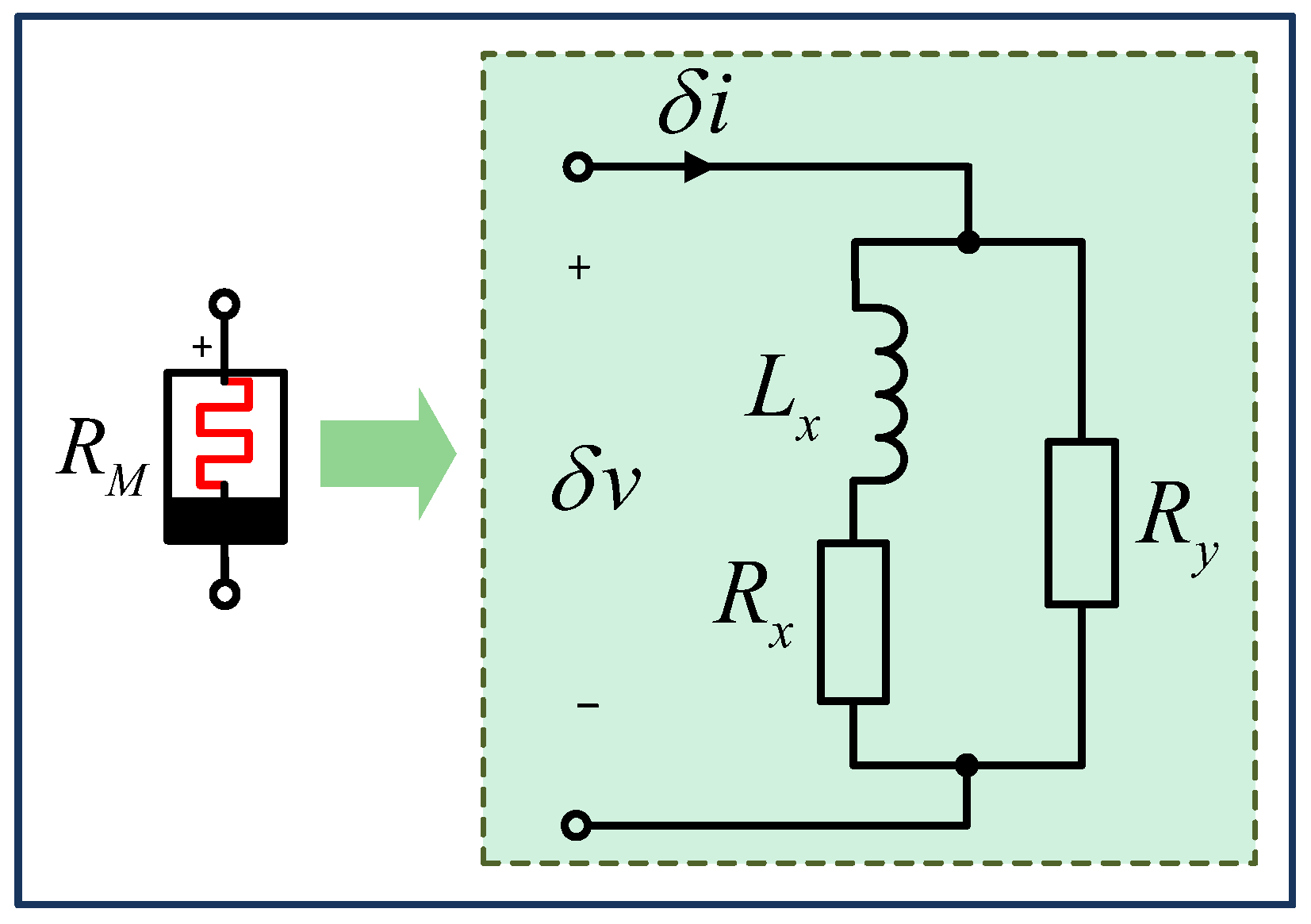
Equation (4a) can be rewritten as:

$$Y_M(s,Q)=\frac{1}{s{L}_x+R_x}+\frac{1}{R_y}$$

(5)

where L_x = 1/(a₁₁b₁₂), R_x = −b₁₁/(a₁₁b₁₂), and R_y = 1/a₁₂. The small-signal equivalent circuit of the SCCM operated in the locally active domains is described in Figure 3.

3.2. Edge of Chaos

When the memristor-based circuits operate at the edge of chaos domain, the operating point must be in the locally active domain and asymptotically stable [1]. According to Equation (4a), the SCCM operates at the locally active domain, i.e., Re Y_M (iω, Q) < 0 for some ω ∈ (−∞, ∞). The SCCM is asymptotically stable only if the real part of the pole of the admittance function is less than zero [2].

The pole and zero of the small-signal admittance in Equation (4a) are calculated as p = b₁₁, and zero z = −(a₁₁b₁₂ − a₁₂b₁₁)/a₁₂, respectively.

From Equation (4a), the frequency response Y_M (iω, Q) of the SCCM is derived, as

$$Y_M(i\omega ,Q)=\frac{a_{11}{b}_{12}}{i\omega -b_{11}}+a_{12}$$

(6a)

where the real part of Y_M (iω, Q) is

$$\mathrm{Re}{Y}_M(i\omega ,Q)=\frac{-b_{11}(a_{11}{b}_{12}-a_{12}{b}_{11})+{\omega }^2{a}_{12}}{b_{11}{}^2+{\omega }^2}=\frac{a_{12}(pz+{\omega }^2)}{b_{11}{}^2+{\omega }^2}$$

(6b)

and the imaginary part is

$$\mathrm{Im}{Y}_M(i\omega ,Q)=\frac{-\omega a_{11}{b}_{12}}{b_{11}{}^2+{\omega }^2}$$

(6c)

Obviously, a₁₂ = 0.01(X² + 0.1) > 0 in Equation (4b). Therefore, if the product of the pole and the zero is less than 0, i.e., pz < 0, the Re Y_M (iω, Q) is negative for the frequency range $-\sqrt{-pz}<\omega <\sqrt{-pz}$.

Both local activity and asymptotic stability are satisfied simultaneously, i.e., pz < 0 and p < 0, calculated z > 0 and p < 0. Therefore, the SCCM operates at the edge of chaos domain if and only if the zero z > 0 and pole p < 0.

The pole and zero of the SCCM are shown in Figure 4, where the edge of chaos domains satisfying zero z > 0 and pole p < 0 are −1 V < V < −0.33 V and 0.33 V < V < 1 V. Because the pole is always less than 0, the locally active domain of SCCM is consistent with the edge of chaos domain of SCCM.

4. SCCM-Based Second-Order Circuit

4.1. Second-Order Circuit

This section will connect an inductor or capacitor with the SCCM to construct a second-order oscillator. The connected inductor or capacitor is determined by judging whether the memristor has capacitive or inductive characteristics.

According to Equations (6b) and (6c), the real and imaginary diagrams of Y_M (iω, Q) of the SCCM over the range −3 × 10³ rad/s < ω < 3 × 10³ rad/s with V = 0.5 V, are shown in Figure 5.

Figure 5 shows that Re Y_M (iω, Q) = 0 S and Im Y_M (iω, Q) = ± 0.25 S at ω = ± 996 rad/s at the locally active domain Ⅰ with V = 0.5 V, which indicates that the SCCM exhibits capacitive characteristic. Hence, an inductor is required to connect with the SCCM to form the oscillator. Based on Chua’s theory [22], the inductance is calculated by L = 1/(ω × Im Y_M (iω, Q)) = 4.02 mH.

Therefore, the second-order circuit is constructed by connecting the SCCM and an inductor, shown in Figure 6.

According to Kirchhoff’s laws, the state equations of the nonlinear system are:

$$\{\begin{array}{l}\frac{dx}{dt}=1000 \left(30-x+|x-20|-|x-40|-10\frac{i_L}{0.01\left(x^2+0.1\right)}\right)\\ \frac{d{i}_L}{dt}=\frac{1}{L}\left(V-\frac{i_L}{0.01\left(x^2+0.1\right)}\right)\end{array}$$

(7)

where x, i_L, and V represent the state variable, the current, and the bias voltage, respectively.

4.2. Complexity Mechanism

From Equation (6a), the composite admittance function Y_S (s, Q) in Figure 6 is described as

$$Y_S(s,Q)=\frac{Y_L{Y}_M(s,Q)}{Y_L+Y_M(s,Q)}=\frac{a_{12}s+a_{11}{b}_{12}-a_{12}{b}_{11}}{a_{12}L{s}^2+(a_{11}{b}_{12}L-a_{12}{b}_{11}L+1) s-b_{11}}$$

(8)

with poles

$$p_1=\frac{-\left(L\left(a_{11}{b}_{12}-a_{12}{b}_{11}\right)+1\right)+\sqrt{{\left(L\left(a_{11}{b}_{12}-a_{12}{b}_{11}\right)+1\right)}^2+4a_{12}{b}_{11}L}}{2a_{12}L}$$

(9a)

and

$$p_2=\frac{-\left(L\left(a_{11}{b}_{12}-a_{12}{b}_{11}\right)+1\right)-\sqrt{{\left(L\left(a_{11}{b}_{12}-a_{12}{b}_{11}\right)+1\right)}^2+4a_{12}{b}_{11}L}}{2a_{12}L}$$

(9b)

When the circuit operates at DC voltage with a frequency of 0 Hz, the inductor is a short circuit. Therefore, the inductor does not affect the DC characteristics of the system. The second-order circuit has the identical DC V–I plot as the SCCM, so their locally active domains are exactly the same.

Then, if the bias voltage V is within the ranges of −1 V < V < −0.33 V and 0.33 V < V < 1 V, the system in Equation (7) is on the locally active domain. The system is asymptotically stable when the real part of two poles p₁ and p₂ of Y_S (s, Q) are less than zero. If these two conditions of local activity and asymptotical stability are satisfied simultaneously, the system is on the edge of chaos domain.

When the bias voltage is 0.5 V on the locally active domain, the Nyquist plots of the poles are shown in Figure 7a over the range 0.6 mH < L < 100 mH.

The Hopf bifurcation point is the intersection of the Nyquist plot with the imaginary axis, referring to the pole where the real part is 0. The stability of the system changes when crossing the Hopf bifurcation point. The system is stable on the left half-plane (LHP) of the Nyquist plot, and the system is unstable on the right half-plane (RHP). In Figure 7a, Hopf bifurcation point is L = 4.02 mH. Therefore, the edge of chaos domain is L < 4.02 mH, the open RHP domain is L > 4.02 mH.

The initial value is set as (5, 0.3). The x − i_L phase diagrams with different inductances of 0.7 mH, 1 mH, 2 mH, 4.02 mH, and 10 mH, are shown in Figure 7b, where dotted trajectories tend to point attractors, and solid trajectories tend to periodic attractors.

Observed that the periodic oscillation generated via the Hopf bifurcation on the RHP Pole domain.

The inductance is set as 4.02 mH. The Nyquist plots of the poles are shown in Figure 8a over the range 0 V < V < 0.92 V. Observed that Hopf bifurcation points are V = 0.5 V and 0.83 V, and the edge of chaos domain is 0 V < V < 0.5 V and 0.83 V < V < 0.92 V.

The initial value is set as (5, 0.3). The x − i_L phase diagrams with different bias voltages of 0.3 V, 0.5 V, 0.7 V, and 0.9 V, are shown in Figure 8b, where dotted trajectories tend to point attractors, and solid trajectories tend to periodic attractors. It follows that the periodic oscillations only occur on the RHP pole domains and the Hopf bifurcation point.

Due to the symmetry, the analysis of the oscillation mechanism of the locally active domains Ⅰ and Ⅱ is similar, so the analysis of the locally active domain Ⅰ is omitted.

According to the above analysis, any parameter domain can be divided into the following three cases:

(i)

Edge of chaos domain (Locally active domain): Re Y(iω, Q) < 0 for some ω ∈ (−∞,∞), and real part of all poles are less than zero.

(ii)

RHP pole domain (Locally active domain): Re Y(iω, Q) < 0 for some ω ∈ (−∞,∞), and there are poles with real parts less than zero.

(iii)

Locally passive domain: Re Y(iω, Q) > 0 for all ω ∈ (−∞,∞).

Then, the domains distribution map of these three domains in the V–L plane is shown in Figure 9.

In Figure 9, the locally active domains are located in the bias voltage ranges −1 V < V < −0.33 V and 0.33 V < V < 1 V, in which the edge of chaos domains are painted green areas and the RHP pole domains are painted yellow areas. The locally passive domains are painted to blue areas with no oscillation. The black lines are the Hopf bifurcation lines, which are the dividing line of the edge of chaos domains and the RHP pole domains. Observed that the symmetrical oscillation occurs on the RHP pole domain of the locally active domain.

Observe from Figure 9 that the oscillation can only appear either on or near the edge of chaos domain in the locally active domains.

4.3. Symmetric Dynamics

The SCCM-based second-order circuit with two symmetrical locally active domains will generate symmetric oscillation. The inductance L is still set as 4.02 mH. The bias voltages are chosen to be ±0.4 V, ±0.5 V, and ±0.6 V located at the edge of chaos domain, Hopf bifurcation line, and RHP pole domain, respectively.

When V = ±0.4 V, ±0.5 V, and ±0.6 V, respectively, the time-domain waveforms and the symmetric phase orbit diagrams are shown in Figure 10, where the blue and red orbit diagrams represent V < 0 V and V > 0 V, respectively. The second-order circuit generates the point attractor oscillation with V = ±0.4 V, and the periodic attractor oscillation with V = ±0.5 V and ±0.6 V.

In Section 4.1, we calculated that the Hopf bifurcation point is inductance L = 4.02 mH with bias voltage V = 0.4 V and frequency f = 996 rad/s. The corresponding time-domain waveforms and phase orbit diagrams are shown in Figure 10c,d, in which the oscillation frequency is 997 rad/s, verifying the prediction of Hopf bifurcation.

5. SCCM-Based Third-Order Circuit

To reveal the oscillation mechanism of chaos [36], an SCCM-based third-order circuit is built by paralleling a capacitor to the SCCM in the second-order circuit, as shown in Figure 11.

According to Kirchhoff’s laws, the state equations of the system in Figure 11 are:

$$\{\begin{array}{l}\frac{dx}{dt}=1000 \left(30-x+|x-20|-|x-40|-10v_C\right)\\ \frac{d{i}_L}{dt}=\frac{1}{L}\left(V-v_C\right)\\ \frac{d{v}_C}{dt}=\frac{1}{C}\left(i_L-0.01\left(x^2+0.1\right)\right)\end{array}$$

(10)

where x, i_L, v_C, and V represent the state variable, inductor current, capacitor voltage, and the bias voltage, respectively.

The inductance is set as 7.2 mH, and the capacitance is set as 10 μF. The initial value (x, i_L, v_C) is (0, 0, 0). The phase diagrams of the system (10) with V = ±0.92 V are shown in Figure 12, which are chaotic oscillations with Lyapunov value LE₁ = 204.5, LE₂ = 0.123, and LE₃ = −4260.3.

5.1. Complexity Mechanism

From Equation (8), the composite admittance function Y_T (s, Q) of the third-order circuit shown in Figure 11 is derived as

$$\begin{array}{l}{Y}_T(s,Q)=\frac{Y_L\left(Y_C+Y_M(s,Q)\right)}{Y_L+Y_C+Y_M(s,Q)} \\ { }_{ }{}_{ }=\frac{C{s}^2+\left(a_{12}-b_{11}C\right)s+\left(a_{11}{b}_{12}-a_{12}{b}_{11}\right)}{CL{s}^3+\left(a_{12}-b_{11}C\right)L{s}^2+\left(1+a_{11}{b}_{12}L-a_{12}{b}_{11}L\right)s-b_{11}}\\ {}_{ }{ }_{ }=\frac{k_1(s-z_1)(s-z_2)}{k_2(s-p_1)(s-p_2)(s-p_3)}\end{array}$$

(11)

where the z₁ and z₂ are the zeros of the composite admittance; the p₁, p₂, and p₃ are the poles of the composite admittance; and the k₁ and k₂ are parameter.

The poles p₁, p₂, and p₃ of the composite admittance function Y_T (s, Q) cannot be derived from the formula, but it can be calculated by MATLAB software.

When the circuit operates at DC voltage with a frequency of 0 Hz, the inductor is equivalent to a short circuit, and the capacitor is equivalent to an open circuit. Therefore, the inductor and capacitor do not affect the DC characteristics of the system. The third-order circuit has the identical DC V–I plot as the SCCM, so their locally active domains are exactly the same.

Then, if the bias voltage V is within the ranges of −1 V < V < −0.33 V and 0.33 V < V < 1 V, the system is on the locally active domain. When these all poles p₁, p₂, and p₃ of Y_T (s, Q) are located in the LHP of Nyquist plot, the system is asymptotically stable. If these two conditions of local activity and asymptotical stability are satisfied simultaneously, the system is on the edge of chaos domain.

When the capacitance is set as 10 μF, the parameter plane V–L of the third-order circuit over the parameter ranges −1.3 V < V < 1.3 V and 0.01 mH < L < 10 mH is divided to three locally passive domains, two symmetrical RHP pole domains, and two symmetrical edge of chaos domains, as shown in Figure 13.

In Figure 13, the locally active domains are located in the bias voltage ranges −1 V < V < −0.33 V and 0.33 V < V < 1 V, in which the edge of chaos domains are painted green areas and the RHP pole domains are painted yellow areas. Observed that the symmetrical periodic oscillation and symmetrical chaos occur on the RHP pole domains. The locally passive domains are painted to blue areas, and the black lines are the Hopf bifurcation lines.

Observe from Figure 13 that the oscillation can only appear either on or near the edge of chaos domain in the locally active domains.

5.2. Symmetric Dynamics

The parameters are set as L = 7.2 mH and C = 10 μF. The initial value (x, i_L, v_C) is set as (0, 0, 0). The bifurcation diagrams and Lyapunov exponent spectrums over the bias voltage ranges −0.96 V < V < −0.86 V and 0.86 V < V < 0.96 V, are shown in Figure 14 a–d, respectively. The minimum Lyapunov exponent value LE₃ is too small and omitted.

In Figure 14a, when V = −0.937 V, the system exhibits complex dynamics from periodic behavior to chaotic behavior. When V > −0.884 V, the chaotic oscillation disappears and gradually evolves into periodic oscillation through the inverse period-doubling bifurcation. The chaotic behaviors of the circuit appear for ranges of −0.937 V < V < −0.884 V and 0.884 V < V < 0.937 V. Observably, the third-order circuit has symmetrical bifurcation behaviors with bias voltage V.

Figure 15a–i show attractors on the x − v_C plane with different bias voltages. The system generates a single cycle with bias voltages of ±0.95 V and −0.87 V. When the bias voltages are ±0.94 V, ±0.938 V, and ±0.93 V, the system will generate double cycle, quadruple cycle, and chaos, respectively. These dynamic behaviors are consistent with those analyzed in Figure 14.

The dynamic behaviors with the capacitance C are visualized by Figure 16a,c, where V = ±0.92 V, L = 7.2 mH, and initial state is (0, 0, 0). The effect of inductance L is visualized by Figure 16b,d, where V = ±0.92 V, C = 10 μF, and initial state is (0, 0, 0). Figure 15a,b show the bifurcation diagram of the capacitor voltage v_C when C ranges from 1 μF to 300 μF and L varies from 6 mH to 9 mH, respectively, where the voltage of the red part is 0.92 V and the blue part is −0.92 V. Figure 15c,d show the Lyapunov exponent spectrums with V = 0.92 V, corresponding to Figure 15a,b, respectively. The minimum Lyapunov exponent value LE₃ is too small and omitted. They are observed that the capacitor voltage v_C has the consistent bifurcation behavior when V = ±0.92 V, which is caused by the symmetry of the system.

To observe the dynamic behaviors varying with the bias voltage V and the capacitance C, we plot the dynamic maps in Figure 17 with the inductance L = 7.2 mH. In Figure 17, the blue, green, and yellow areas represent the chaos, periodic oscillation, and stable point, respectively. In addition, the boundary between the blue area and the green area represents that the dynamic behavior changes from periodic oscillation to chaos or from chaos to periodic oscillation. To observe the chaotic behavior of the third-order circuit, we zoomed in on the region where chaotic oscillations appear.

The locally active domains are −1 V < V < −0.33 V and 0.33 V < V < 1 V. Observed from Figure 17 that the third-order circuit has consistent symmetrical dynamics, and the chaos and periodic oscillation only occur in the locally active domains.

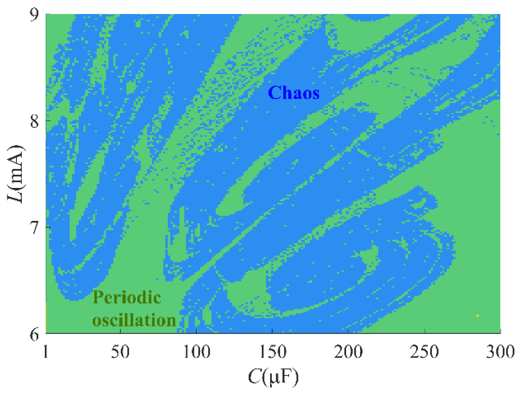
With the bias voltage V = −0.92 V, the dynamic map depending on both the inductance L and capacitance C is shown in Figure 18, where C ranges from 1 μF to 300 μF and L varies from 6 mH to 9 mH. In Figure 18, the blue and green areas represent the chaos and periodic oscillation, respectively. The dynamic map shows the complex behaviors of the periodic oscillation and chaotic oscillation of the third-order system.

6. Conclusions

In this paper, a modified Chua Corsage Memristor is proposed, which has symmetrical locally active domains. The local activity and the edge of chaos of the SCCM are explored by analyzing the small-signal equivalent circuit. By analyzing the small-signal admittance function, the SCCM is determined to exhibit the capacitive characteristic in its locally active domain, so it can be connected with the inductor to form a second-order circuit. The edge of chaos domain is determined using the conjugate poles of the admittance function and local activity. It is proven that the second-order circuit generates complex symmetrical oscillation either on or near the edge of chaos domains. Furthermore, the third-order circuit is built by paralleling a capacitor with the SCCM in the second-order circuit. Based on the theory of local activity and edge of chaos, the oscillation mechanism of the chaos and periodic oscillation in the third-order circuit has been expounded.

The action potential may emerge either on or near the edge of chaos, so the CCM could be used to neuronal circuits to simulate neuromorphic behavior. The research to explore the mechanism of neuromorphic dynamics is of great significance for neurons and even neural networks.

References

- Chua, L.O. Local activity is the origin of complexity. Int. J. Bifurc. Chaos 2011, 15, 3435–3456. [Google Scholar] [CrossRef] [Green Version]
- Ascoli, A.; Slesazeck, S.; Mähne, H.; Tetzlaff, R.; Mikolajick, T. Nonlinear dynamics of a locally-active memristor. IEEE Trans. Circuits Syst. I-Regul. Pap. 2015, 62, 1165–1174. [Google Scholar] [CrossRef]
- Liang, Y.; Wang, G.; Chen, G.; Dong, Y.; Yu, D.; Iu, H.H.C. S-Type Locally active memristor-based periodic and chaotic oscillators. IEEE Trans. Circuits Syst. I-Regul. Pap. 2020, 67, 5139–5152. [Google Scholar] [CrossRef]
- Chua, L.O.; Sbitnev, V.; Kim, H. Neurons are poised near the edge of chaos. Int. J. Bifurc. Chaos 2012, 22, 1250098. [Google Scholar] [CrossRef]
- Chua, L.O. Everything you wish to know about memristors but are afraid to ask. Radioengineering 2015, 24, 319–368. [Google Scholar] [CrossRef]
- Itoh, M.; Chua, L.O. Chaotic oscillation via edge of chaos criteria. Int. J. Bifurc. Chaos 2017, 27, 1730035. [Google Scholar] [CrossRef]
- Chua, L.O. Memristor, Hodgkin–Huxley, and edge of chaos. Nanotechnology 2013, 24, 67–94. [Google Scholar] [CrossRef] [PubMed]
- Pickett, M.D.; Williams, R.S. Sub-100 fJ and sub-nanosecond thermally driven threshold switching in niobium oxide crosspoint nanodevices. Nanotechnology 2012, 23, 215202. [Google Scholar] [CrossRef] [PubMed]
- Li, S.; Liu, X.; Nandi, S.K.; Nath, S.K.; Elliman, R.G. Origin of current-controlled negative differential resistance modes and the emergence of composite characteristics with high complexity. Adv. Funct. Mater. 2019, 29, 1905060. [Google Scholar] [CrossRef] [Green Version]
- Kumar, S.; Williams, R.S. Separation of current density and electric field domains caused by nonlinear electronic instabilities. Nat. Commun. 2018, 9, 2030. [Google Scholar] [CrossRef] [PubMed] [Green Version]
- Goodwill, J.M.; Ramer, G.; Li, D.; Hoskins, B.D.; Pavlidis, G.; McClelland, J.J.; Centrone, A.; Bain, J.A.; Skowronski, M. Spontaneous current constriction in threshold switching devices. Nat. Commun. 2019, 10, 1628. [Google Scholar] [CrossRef] [PubMed]
- Dong, Y.; Wang, G.; Chen, G.; Shen, Y.R.; Ying, J.J. A bistable nonvolatile locally-active memristor and its complex dynamics. Commun. Nonlinear Sci. Numer. Simul. 2020, 84, 105203. [Google Scholar] [CrossRef]
- Ying, J.; Liang, Y.; Wang, J.; Dong, Y.; Wang, G.; Gu, M. A tristable locally-active memristor and its complex dynamics. Chaos Solitons Fract. 2021, 148, 111038. [Google Scholar] [CrossRef]
- Sharma, A.A.; Bain, J.A.; Weldon, J.A. Phase coupling and control of oxide-based oscillators for neuromorphic computing. IEEE J. Explor. Solid-State Comput. Devices Circuits 2015, 1, 2329–9231. [Google Scholar] [CrossRef]
- Zhang, X.; Zhuo, Y.; Luo, Q.; Wu, Z.; Midya, R.; Wang, Z.; Song, W.; Wang, R.; Upadhyay, N.K.; Fang, Y.; et al. An artificial spiking afferent nerve based on Mott memristors for neurorobotics. Nat. Commun. 2020, 11, 51. [Google Scholar] [CrossRef] [Green Version]
- Kumar, S.; Strachan, J.P.; Williams, R.S. Chaotic dynamics in nanoscale NbO2 mott memristor for analogue computing. Nature 2017, 548, 318–321. [Google Scholar] [CrossRef]
- Ying, J.; Liang, Y.; Wang, G.; Iu, H.H.C.; Zhang, J.; Jin, P. Locally active memristor based oscillators: The dynamic route from period to chaos and hyperchaos. Chaos 2021, 31, 063114. [Google Scholar] [CrossRef]
- Dong, Y.; Wang, G.; Liang, Y.; Chen, G. Complex dynamics of a bi-directional N-type locally-active memristor. Commun. Nonlinear Sci. Numer. Simul. 2022, 105, 106086. [Google Scholar] [CrossRef]
- Mannan, Z.I.; Choi, H.; Kim, H. Chua corsage memristor oscillator via Hopf bifurcation. Int. J. Bifurc. Chaos 2016, 26, 1630009. [Google Scholar] [CrossRef]
- Mannan, Z.I.; Yang, C.; Kim, H. Oscillation with 4-lobe Chua corsage memristor. IEEE Circuits Syst. Mag. 2018, 18, 14–27. [Google Scholar] [CrossRef]
- Mannan, Z.I.; Yang, C.; Adhikari, S.P.; Kim, H. Exact analysis and physical realization of the 6-lobe Chua corsage memristor. Complexity 2018, 2018, 8405978. [Google Scholar] [CrossRef]
- Mannan, Z.I.; Choi, H.; Rajamani, V.; Kim, H.; Chua, L.O. Chua corsage memristor: Phase portraits, basin of attraction, and coexisting pinched hysteresis loops. Int. J. Bifurc. Chaos 2017, 27, 1730011. [Google Scholar] [CrossRef]
- Etemadi, M.; Ghobaei-Arani, M.; Shahidinejad, A. Resource provisioning for IoT services in the fog computing environment: An autonomic approach. Comput. Commun. 2020, 161, 109–131. [Google Scholar] [CrossRef]
- Aslanpour, M.S.; Dashti, S.E.; Ghobaei-Arani, M.; Rahmanian, A.A. Resource provisioning for cloud applications: A 3-D, provident and flexible approach. J. Supercomput. 2018, 74, 6470–6501. [Google Scholar] [CrossRef]
- Zhang, W.; Li, C.D.; Huang, T.W.; He, X. Synchronization of memristor-based coupling recurrent neural networks with time-varying delays and impulses. IEEE Trans. Neural Netw. Learn. Syst. 2015, 26, 3308–3313. [Google Scholar] [CrossRef]
- Vadivel, R.; Ali, M.S.; Joo, Y.H. Robust H∞ performance for discrete time T-S fuzzy switched memristive stochastic neural networks with mixed time-varying delays. J. Exp. Theor. Artif. Intell. 2021, 33, 79–107. [Google Scholar] [CrossRef]
- Kumar, S.; Williams, R.S.; Wang, Z. Third-order nanocircuit elements for neuromorphic engineering. Nature 2020, 585, 518–523. [Google Scholar] [CrossRef]
- Yi, W.; Tsang, K.K.; Lam, S.K.; Bai, X.; Crowell, J.A.; Flores, E.A. Biological plausibility and stochasticity in scalable VO2 active memristor neurons. Nat. Commun. 2018, 9, 4661. [Google Scholar] [CrossRef]
- Dong, Y.J.; Liang, Y.; Wang, G.Y.; Iu, H.H.C. Chua corsage memristor based neuron models. Electron. Lett. 2021, 57, 903–905. [Google Scholar] [CrossRef]
- Jin, P.P.; Wang, G.Y.; Liang, Y.; Iu, H.H.C.; Chua, L.O. Neuromorphic dynamics of Chua corsage memristor. IEEE Trans. Circuits Syst. I-Regul. Pap. 2021, 68, 4419–4432. [Google Scholar] [CrossRef]
- Dogaru, R.; Chua, L.O. Edge of chaos and local activity domain of FitzHugh–Nagumo equation. Int. J. Bifurc. Chaos 1998, 8, 211–257. [Google Scholar] [CrossRef]
- Li, C.; Min, F.; Li, C. Multiple coexisting attractors of the serial–parallel memristor-based chaotic system and its adaptive generalized synchronization. Nonlinear Dyn. 2018, 94, 2785–2806. [Google Scholar] [CrossRef]
- Peng, G.; Min, F. Multistability analysis, circuit implementations and application in image encryption of a novel memristive chaotic circuit. Nonlinear Dyn. 2017, 90, 1607–1625. [Google Scholar] [CrossRef]
- Chua, L.O.; Kang, S.M. Memristive devices and systems. Proc. IEEE 1976, 64, 209–223. [Google Scholar] [CrossRef]
- Corinto, F.; Ascoli, A. Memristive diode bridge with LCR filter. Electron. Lett. 2012, 48, 824–825. [Google Scholar] [CrossRef]
- Yuan, F.; Li, Y. A chaotic circuit constructed by a memristor, a memcapacitor and a meminductor. Chaos 2019, 29, 101101. [Google Scholar] [CrossRef] [PubMed]
Figure 1.
Pinched hysteresis loops of the SCCM when the input voltage signals v(t) = sin (2πft).
Figure 2.
DC V–I plot of the SCCM.
Figure 3.
The small-signal equivalent circuit of the SCCM.
Figure 4.
Zero and pole diagrams of YM (s, Q) of the SCCM.
Figure 5.
The real and imaginary diagrams of YM (iω, Q) of the SCCM versus frequency ω at V = 0.5 V.
Figure 6.
The SCCM-based second-order circuit.
Figure 7.
(a) The Nyquist plots of the poles over the range 0.6 mH < L < 100 mH. (b) The x − iL phase diagrams with different inductances of 0.7 mH, 1 mH, 2 mH, 4.02 mH, and 10 mH.
Figure 8.
(a) The Nyquist plots of the poles over the range 0 V < V < 0.92 V. (b) The x − iL phase diagrams with different bias voltages of 0.3 V, 0.5 V, 0.7 V, and 0.9 V.
Figure 9.
Domains distribution map in the V–L plane over the ranges −1.3 V < V < 1.3 V and 0.01 mH < L < 10 mH.
Figure 10.
(a) Symmetric oscillations of the second-order circuit. (a,c,e). The time-domain waveforms with V = ±0.4 V, ±0.5 V, and ±0.6 V, respectively. (b,d,f). The x − iL phase diagram with V = ±0.4 V, ±0.5 V, and ±0.6 V, respectively.
Figure 11.
The SCCM-based third-order circuit.
Figure 12.
Chaotic oscillation of the third-order circuit with V = ± 0.92 V. (a) x − iL plane. (b) x –uC plane. (c) iL − uC plane. (d) x − iL − uC plane.
Figure 13.
Figure 14.
(a,b). The bifurcation diagrams over the ranges −0.96 V < V < −0.86 V and 0.86 V < V < 0.96 V. (c,d). The corresponding Lyapunov exponent spectrums.
Figure 15.
The oscillation attractors with different bias voltage V of (a) −0.95 V, (b) −0.94 V, (c) −0.938 V, (d) −0.93 V, (e) −0.87 V, (f) 0.93 V, (g) 0.938 V, (h) 0.94 V, and (i) 0.95 V.
Figure 16.
The dynamics behaviors over the capacitance range 0.1 μF < C < 300 μF: (a) the bifurcation diagram with bias voltage ± 0.92 V, and (b) the Lyapunov exponent spectrum with bias voltage 0.92 V. The dynamics behaviors over the inductance range 6 mH < C < 9 mH: (c) the bifurcation diagram with bias voltage ± 0.92 V, and (d) the Lyapunov exponent spectrum with bias voltage 0.92 V.
Figure 17.
The dynamic map over the ranges 1 μF < C < 300 μF and −1.3 V < V < 1.3 V.
Figure 18.
The dynamic map over the ranges 1 μF < C < 300 μF and 6 mH < L < 9 mH.
Publisher’s Note: MDPI stays neutral with regard to jurisdictional claims in published maps and institutional affiliations. |
© 2022 by the authors. Licensee MDPI, Basel, Switzerland. This article is an open access article distributed under the terms and conditions of the Creative Commons Attribution (CC BY) license (https://creativecommons.org/licenses/by/4.0/).
Share and Cite
MDPI and ACS Style
Ying, J.; Liang, Y.; Li, F.; Wang, G.; Shen, Y. Complex Oscillations of Chua Corsage Memristor with Two Symmetrical Locally Active Domains. Electronics 2022, 11, 665. https://doi.org/10.3390/electronics11040665
AMA Style
Ying J, Liang Y, Li F, Wang G, Shen Y. Complex Oscillations of Chua Corsage Memristor with Two Symmetrical Locally Active Domains. Electronics. 2022; 11(4):665. https://doi.org/10.3390/electronics11040665
Chicago/Turabian StyleYing, Jiajie, Yan Liang, Fupeng Li, Guangyi Wang, and Yiran Shen. 2022. "Complex Oscillations of Chua Corsage Memristor with Two Symmetrical Locally Active Domains" Electronics 11, no. 4: 665. https://doi.org/10.3390/electronics11040665
Note that from the first issue of 2016, this journal uses article numbers instead of page numbers. See further details here.