Abstract
This paper presents an overview and formalization of the Functional Mock-up Interface (FMI) 3.0. The formalization captures the new FMI 3.0 standard and is intended to be used as an introduction for conceptualizing the use of clocks in the FMI standard to support the simulation of event-based cyber-physical systems. The FMI 3.0 standard supports two kinds of clock-based simulations: Synchronous Clocked Simulation to ensure predictable systems scheduling with multiple simultaneous events and scheduled execution to facilitate real-time simulations comprising multiple black-box models by allowing fine-grained control over the computation time of submodels. The formalization is a basis for developing tools for orchestrating, verifying and validating the composition of multiple FMUs. The formalization is provided as an accessible VDM-SL specification.
1. Introduction
Modern cyber-physical systems (CPSs), such as, e.g., nuclear power plants, cars, and airplanes, consist of cyber components (a controller) and physical components (a plant) [1]. Modeling a CPS often spans different paradigms, including continuous-time, modal models, and discrete events. Moreover, each subsystem is typically developed by different specialized companies using different tools and formalisms [2].
As more and more Modeling and Simulation (M&S) tools are used in system-engineering processes, it becomes clear that standards are needed to improve the interoperability of such tools. The Functional Mock-up Interface (FMI) standard [3] aims to enable the exchange and cooperative simulation of black-box models. Version 2.0 of the standard strikes a balance between supporting the most common features across the plethora of M&S tools and enabling efficient simulations of continuous systems. Its wide adoption with more than 170 tools supporting the standard [4] has, however, placed pressure in supporting two important use cases: simulation scenarios where time-based and state events play a frequent role in synchronizing a subset of the participating models (e.g., controller code with tasks running at different rates); and scenarios where the goal is to control the computation time of the different models, so that a real-time co-simulation can be achieved.
Developers of such systems have historically turned to other formalizations such as Modelica [5], HLA [6] and DEVS [7,8] for simulation and modeling of such event-driven systems since they support a natural mechanism for modeling and simulating continuous systems with discrete events.
As the name suggests, DEVS (Discrete-Event System Specification) is a formalism for modeling discrete-event systems composed of discrete-event submodels. DEVS lets subcomponents trigger events on state transitions and propagate them to others using connections between subcomponents. HLA (High-Level Architecture) is a modeling language for discrete-event-based systems that greatly facilitates geographically distributed simulations and provides, in contrast to FMI, a standardized run-time infrastructure (RTI) to handle information exchange and synchronization between the different components. There have been several attempts to integrate the previous FMI versions (and other simulation standards) into HLA to leverage the benefits of the standardized RTI [9,10,11,12] to exchange data and synchronize events between FMUs. Nevertheless, these approaches are not standardized and do not provide a formal semantics for the interaction between FMUs and the RTI of HLA. Furthermore, these approaches do not provide the same fine-grained control over the simulation as the FMI 3.0 standard. In the continuous time paradigm, the Modelica language enables one to model an event-driven behavior using synchronous clocks. Synchronous clocks are inspired by synchronous languages [13] that include clocks to give the developers a fine-grained control over the execution of the simulation while still having well-defined formal semantics. Synchronous clocks are Boolean variables represented as input and output ports associated with a set of equations to be evaluated at each clock tick. The ability to link equations directly to ports provides the user with a fine-grained simulation control. Synchronous clocks can furthermore be connected to model events spanning multiple components, and a similar concept of clocks has been recently introduced in the Modelica language version 3.3 [5].
Despite the success and popularity of these formalisms, they make it difficult to couple simulations of models produced in different tools, to protect their Intellectual Property (IP), and to handle models with algebraic loops:
- HLA and DEVS: support a very elegant mechanism to handle discrete events, nevertheless it is complicated to incorporate efficient methods to solve algebraic loops that span multiple simulation units. This means that such formalisms are not suitable to simulate systems containing such feedback mechanisms (see [14] for more details).
- FMI 2.0: supports an efficient simulation of continuous systems, including algebraic loops spanning multiple FMUs. However, its fundamental event mechanism does not allow one to easily model multi-rate and real-time systems (which are more natural in HLA and DEVS), where the orchestration of the system should adapt according to the state of the system.
It is to address the above limitations that the FMI version 3.0 SC [15] has been proposed: it supports the implementation of Synchronous Clocked (SC) co-simulations. FMI 3.0 extends the FMI 2.0 standard with the notion of clocks to provide an already efficient method to conduct continuous-time co-simulations with a more elaborate notion of events. The clocks are used to define the simulation unit reaction to specific time-based and event-based behavior similarly to synchronous clocks in the Modelica language [5]. This enables co-simulation practitioners to use FMI 3.0 standard to co-simulate systems with a more complex interaction mechanism and to model systems with real-time behavior.
- Contribution
This paper gives an overview of the FMI 3.0 support for two kinds of clock-based simulations: Synchronous Clocked Simulation (SC) and Scheduled Execution (SE). The paper provides a formal semantics of the two simulation modes, which tool vendors and practitioners can use to implement and understand the new features of the FMI 3.0 standard. Synchronous Clocked Simulation aims at scenarios where the cause and exact time of multiple simultaneous events can be unambiguously conveyed. At the same time, scheduled execution facilitates real-time simulation among black-box models by giving practitioners a fine-grained control (compared to version 2.0 of the FMI standard) over when specific tasks inside the black-box simulation unit can be executed.
1.1. Prior Work
This manuscript extends a prior paper [16] by introducing a formal semantics of the FMI 3.0 standard. The formal semantics allow tool vendors and practitioners to obtain a uniform and unambiguous understanding of the FMI 3.0 standard.
1.2. Structure
The next section introduces the common concepts and the interface elements that are common to SC and SE. Section 3 details SC, along with a motivating example. Section 4 focuses on SE, following the same structure as Section 3. In Section 5, we discuss some of the related works, and in Section 6 we summarize and conclude.
2. Common Interface and Concepts
This section introduces the concept of co-simulation, and gives an informal overview of the different types of clocks and interfaces of FMI 3.0.
Co-simulation is a technique to combine multiple black-box simulation units to compute the combined models’ behavior as a discrete trace. Simulation units are combined by coupling outputs of one simulation unit to inputs of another to denote data dependencies between the models. See [14,17], for an introduction. The simulation units, often developed and exported independently from each other in different M&S tools, are coupled using an orchestration algorithm, often developed independently as well, that communicates with each simulation unit via its interface. This interface, an example of which is the FMI standard interface for co-simulation, comprises functions for setting/getting inputs/outputs and computing the associated model behavior over a given time interval.
The FMI 3.0 defines three interface types: the Co-Simulation (CS), the Model Exchange (ME), and the Scheduled Execution (SE). A simulation unit is in the context of FMI called a Functional Mock-up Unit (FMU), implementing one or more of the three interfaces. An FMU is a zip containing: binaries and/or source code implementing the API functions; miscellaneous resources; and an XML file called the modelDescription, describing the variables, model structure, and other metadata of the FMU.
For each interface type, the FMU may implement optional features, such as declaring synchronous clocks (in the case of ME or CS), or scheduled execution clocks (in the case of SE). Figure 1 summarizes the different interface types and the main concepts relevant to this paper. All three interfaces (CS, ME, and SE) share common functionality, such as the declaration and usage of variables and clocks.
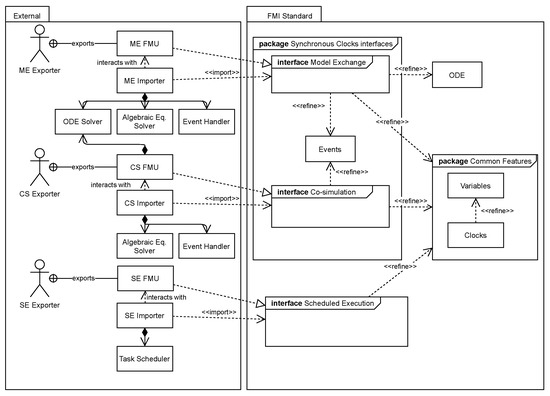
Figure 1.
Overview of relevant concepts. Please note that there might be domain-specific importers which do not need an ODE solver because the supported FMUs do not contain continuous variables. This figure attempts to illustrate the most common differences between the interface types.
The differences between the three interface types can be seen on the left-hand side of Figure 1. The importer is the software that imports the FMU and interacts with the FMUs through their interfaces. We distinguish between three importers, each corresponding to one of the interface types, and each with different responsibilities. The ME importer often needs to provide a differential equation (ODE) solver to compute the behavior of the model and be able to handle events. In contrast, the CS importer does not need to provide an ODE solver, because such a solver can be implemented inside the CS FMU. Finally, the SE importer provides a task scheduler to determine precisely when each task implemented in the FMU will be executed.
The ME and CS both contain mechanisms to communicate events to the importer, and, as we detail later, both enable Synchronous Clocked (SC) simulation.
Broadly speaking, a simulation involving multiple connected FMUs goes through the following simulation modes. Note that this is a simplification of the states or modes defined in the state diagrams of the FMI 3.0 standard:
- Initialize—The FMUs are instantiated and their initial state/inputs/outputs/parameters are calculated or set by the importer.
- Step—The simulation is progressing in simulated time, and FMUs that represent ODEs are being numerically integrated.
- Event—The simulated time is stopped and events (e.g., clock ticks, parameter changes) are being processed.
- Terminate—The simulation has finished, and all resources are freed.
The Step and Event modes come after the Initialize mode and are interleaved.
In the following sub-sections, we introduce FMI 3.0 clocks. We specify how they are declared, connected, and interacted with, as well as common constraints imposed by the standard. These characteristics about clocks are common to the SC and SE clock interpretations.
2.1. Clock Taxonomy
Clocks represent an abstraction of activities whose occurrence is tied to specific points in time or specific states. They appear in many modeling formalisms for systems that interact with the real world [5,13], where it is crucial to represent computations that happen at different rates or as a result of conditions observed in the environment. Conceptually, each clock represents a sequence of instants in time where the clock is active, called ticks. From the entities that can interact with a clock, we highlight the FMU and the importer (recall Figure 1). The FMU is the entity that declares and implements the behavior associated with a given clock, while the importer is the entity that interacts with the clock. The activation status of an input clock is determined by the importer, while the FMU itself determines the activation status of an output clock.
Clocks are declared in the modelDescription file and can be seen as a special variable type. Each clock has specific attributes, among others, an identifier called the value reference, a causality attribute (whether the clock is an input or output, as we will discuss later), and an attribute intervalVariability (declaring the type of clock discussed later). Dynamically, during the simulation, each clock can be either active or inactive (denoted as the clock’s state). Depending on the clock type and causality, the importer can set or obtain the state of a clock (see below).
There are two main types of clocks: time-based and triggered. Time-based clocks are associated with an interval. The interval dictates the time duration (in simulated time units) between the last tick and the next tick at any moment in simulated time. Such intervals can be queried or set by the importer, depending on the clock’s interval attribute (see below). In contrast, triggered clocks have no a priori known interval. The FMU or importer must set/get the (activation) state of the clock depending on the system’s state. The importer can activate a triggered input clock to tell the FMU about a change to the system caused by one of the other FMUs. In comparison, an FMU can activate an output clock to highlight an internal event to the rest of the system. The different clock types are listed in Table 1 according to who calculates the intervals and ticks the clock.

Table 1.
Overview of clock types and their attributes.
Before discussing the causality of clocks, it is important to distinguish between the entity that dictates the clock interval and the entity that activates the clock. This distinction is important in the context of the FMI because the simulated time is a real-valued quantity, represented by a finite-resolution variable. For example, the FMU may declare the interval of a periodic clock in the XML, but it is the importer that will decide exactly at which simulated time the input clock ticks. Due to numerical inaccuracies, it may happen that the interval (in simulated time) between clock ticks does not match exactly the interval declared by the FMU.
Time-based clocks are always input clocks since it is the importer who is responsible for activating the clock (even though the clock interval can be decided by other entities, as shown in Table 1). On the other hand, triggered clocks can be input or output clocks. The importer is responsible for setting the activation state of the triggered input clock. In contrast, the FMU controls the activation state of its output clocks; the importer can query these output clocks to observe their state. The causality, therefore, plays a role in determining how clocks can be connected and how they can be activated.
2.2. Clock Variables and Dependencies
An output clock can be connected to an input clock, just as a “normal” output port can be connected with a “normal” input port. It is also possible to connect two input clocks to the same clock source or even have one input clock connected to two different output clocks. A connection from clock to clock means that whenever clock ticks, then clock should also tick. For triggered clocks, that is relatively easy to enforce: whenever an output clock activates, the connected input clock should be activated. For time-based clocks, the importer must take into account the intervalVariability attributes of the clocks and decide whether such a connection makes sense or not.
FMUs can declare internal dependencies referred to as feedthrough between their output and input variables in the modelDescription file. An output variable y depends on an input variable u when the computation of y’s value requires the value of u is computed at the same simulated time instance. For example, in Figure 2, the output port is computed from, among other dependencies, the input port . Please note that we denote input variables both normal ports and clocks with u and output variables with y.
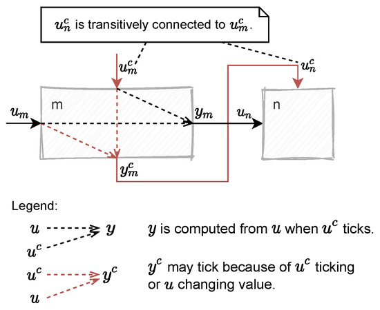
Figure 2.
Example clock connections and dependencies. The symbols m and n refer to FMUs.
An output clock can also depend on one or more input clocks or variables. The meaning is that the state of such input clocks or the value of the input variables is taken into account when deciding whether the output clock will tick. For example, in Figure 2, the output clock may tick when the input clock ticks, or because of a change on the input port . It is not necessarily the case that will tick whenever an input clock, that depends on, ticks.
When a clock ticks (we use to denote a clock when its causality is irrelevant), there is a set of variables whose values should be computed. We denote this set of variables by “’s variables” or “clocked variables” when the specific clock is unimportant. FMI imposes few constraints on the clocked variables. However, the FMU can declare in its modelDescription, for each variable which clocks it depends on (usually not more than one) using the attribute clocks. For example, in Figure 2, is computed when ticks. Clocked variables can only be accessed when their associated clock is ticking; accessing the variables of clock ’s when is not ticking is undefined behavior. Please note that an output clock can be a clocked variable that only can be accessed when its associated clock is ticking. This can introduce cyclic dependencies between multiple clocks, which we must avoid for all scenarios to achieve meaningful simulations. Clocked variables are introduced to give the user a fine grain of control over the simulation because it allows the user to specify precisely using the clocks attribute which variables need to be exchanged/recomputed when a specific clock ticks.
3. Synchronous Clocked Simulation
This section describes the Synchronous-Clock (SC) interpretation of the clocks interface introduced in the previous section. This interpretation is inspired by the clock’s implementation in the Modelica specification [5] and existing synchronous-clock theories such as [13]. Nevertheless, it is adapted to reflect the constraints of black-box co-simulation. As such, we offer no guarantees of semantic equivalence.
We start by detailing the main simulation modes for CS and ME as if no clocks were declared. To focus on the essential mechanisms, we abstract away from the ME and CS interfaces and present them in a unified manner using set-theoretic constructs while referring the reader to the FMI standard for more details.
3.1. Background on CS and ME
Following the superdense time formulation as in [18], the simulation time is a tuple where . In Step mode, the real part of time is increasing and ; during Event mode, the integer part of time is increasing while is held constant. Figure 3 illustrates a possible trajectory for the values of a variable v in superdense time from the importer’s perspective in Figure 3b which only can inspect the variable v at discrete points in time. The continuous evolution of v is represented in Figure 3a. The Step mode produces a continuous evolution of v, while the Event mode introduces discontinuities in the calculation of v. Figure 3 also illustrates that the resolution/step size of the simulation time is not uniform across the simulation; the first step is of size 0.7 and the second step is of size 1.3.
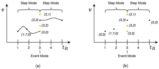
Figure 3.
An example of the variable trajectory of the variable v in superdense time. The continuous evolution of v is represented in (a) as a line. The dots on the line represent the variable’s value and the time points at which the variable v can be inspected. The yellow dots denote that the FMU is in Event mode, while the black dots denote that the FMU is in Step mode. The evolution of v from the importer’s perspective is represented in (b) as a set of discrete points. (a) Trajectory of the variable v in superdense time. (b) Trajectory of the variable v from the importer’s perspective.
We distinguish between discrete and continuous variables. Continuous variables are those whose value changes continuously over time; a continuous variable can be defined as a function of time, meaning it can only take a specific value at a given time . Discrete variables are those whose value changes only at discrete points in time; discrete variables can take multiple values at the same real part of time in Event mode. The different values of a discrete variable can be distinguished by the integer part of time . We define the following relations (= and <) between superdense time instances.
In Step mode, the FMU and importer cooperate in approximating the solution of a system of differential equations described by the FMU. An example of this can be seen in Figure 3a where the value of variable v is the approximated solution to such a system of differential equations. In the case of ME, the FMU provides the derivatives, and the importer provides the inputs and solver. In CS, the importer provides the inputs, and the FMU provides the derivatives and solver (recall Figure 1).
The importer may switch the FMU to Event mode if one or more of the following situations occur. Note that there are other kinds of events, but for simplicity, we highlight the main ones:
- Time events—the simulated time reached a specific point in time where an event is happening (a clock is ticking). The time was known at the end of the last Event mode;
- State events—The value of some variable crossed a threshold that is known to the FMU;
- Input events—The value of an input variable changed discretely, introducing a discontinuity.
The mechanism for detecting and communicating the occurrence of events is described in FMI 3.0 [15] for both the ME and CS interfaces, so we will not discuss these mechanisms here. It suffices to assert that the importer can determine that the FMU should switch to Event mode at the appropriate simulated time.
During Event mode, the FMUs and importer cooperate in solving a set of algebraic equations associated with the event that triggered the Event mode. To solve the equations, the importer will typically construct a dependency graph between the output and input variables, using the model structure declared by the FMU [19]. The FMU may be part of a larger simulation model (scenario), where its inputs can depend on both external entities as well as its own outputs. Therefore, the dependency graph may involve not just the FMU variables but other relevant external variables. As a result, there might exist cyclic dependencies between variables of the FMU. These manifest as non-trivial strongly connected components in the dependency graph [20], indicating that the system is represented as a non-linear equation that must be solved using traditional solution techniques [14]. The importer solves such a system by setting and querying the variables of the FMU. At the same time, the FMU recomputes any output variable that might change due to new input values set by the importer. The critical consequence is that all variables of the FMU have acquired a value that stabilizes the system of equations.
The FMU may remain in Event mode, and perform a new iteration to handle new events. These new events may be caused by the importer or by a new value for some variable. The FMI defines the mechanism by which the FMU or importer agrees that a new event iteration is needed. Each new event iteration corresponds to one increment in the integer part of the superdense simulated time. If no more event iterations are needed, Event mode is finished and the FMU returns to Step mode.
Please note that in Event mode, as part of the procedure to solve non-linear equations, there may be hundreds of iterations to converge and obtain a solution. These intermediate values are not shown in Figure 3 and do not cause the integer part of the superdense time to increment because they happen within one superdense time instant. Therefore in Figure 3 there are three event handling iterations. When switching back to Step mode, the FMU informs the importer of the next time-based event (if such event is defined).
3.2. Limitations of FMI 2.0: Discerning Events
The basic event signaling mechanism offered by FMI 2.0 is adequate for most applications without simultaneously occurring events. However, they are insufficiently expressive for simulations with many simultaneous events. We illustrate this with a simple example shown in Figure 4, devised to motivate the need for clocks. The example shows a closed-loop control system, where the CtrlFMU is specified as an FMU, and the remaining submodels are specified in some other language. We sketch the CtrlFMU equations, but, note that the importer has no access to these (it can only query the FMU for the values of the output variables). The CtrlFMU, every seconds (we abuse the notation r to denote both a clock r and its frequency), obtains a sample from the Plant (produced by the Sensor), and calculates its next state, based on the previous state pre(u_r), the sampled value x_r, and some dynamic configuration parameter a that is calculated by the Supervisor. The latter, depending on the Plant dynamics (the sampling rate of which we ignore) may decide to reconfigure the Controller.
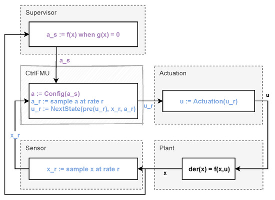
Figure 4.
Motivating example with supervisor controller.
Using only the basic event mechanism of FMI 2.0, it is cumbersome to simulate the scenario in Figure 4, for the following reasons:
- It is not possible to let the CtrlFMU control the sampling rate of the system (r) based on the state of the system. Instead, we must use a fixed sampling rate h to decide when the importer should exchange values between the Plant and the CtrlFMU. The importer only receives information about the next time event, after each Event mode of the CtrlFMU.
- There is no way for the CtrlFMU to know which equations to compute during an Event mode. For example, the CtrlFMU must rely on approximate floating-point comparisons to figure out if it should compute the Config equation or not. Conversely, when a new sample x_r is available and the x_s is unchanged, the CtrlFMU must know that the Config equation must remain disabled.
- The Importer cannot infer which values it makes sense to exchange during an Event mode. Instead, it must exchange all values that are relevant to the system, which will result in a lot of redundant data exchange and a slow simulation.
Figure 5 shows how clocks address the limitations highlighted by the example in Figure 4. By introducing a triggered input clock s and a time-based input clock r, it is clear who is responsible for the unambiguous activation of the clocks. The Supervisor controls the triggered clock s, and the importer controls the time-based clock r. The clocks define a set of variables/equations to be solved when the clock ticks. This means no approximate floating-point comparisons are needed to know which equations to solve when entering Event mode. The importer can therefore infer from the set of active clocks which values it makes sense to exchange during an Event mode.
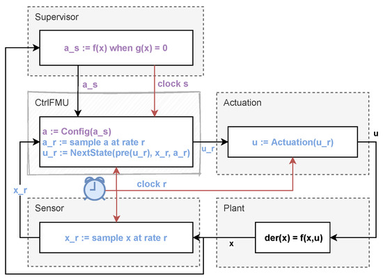
Figure 5.
Clocked version of Figure 4.
We have motivated the need for synchronous clocks and will now describe the semantics of the SC interface described in the FMI standard [15]. However, we need to introduce some terminology and notation first.
3.3. Notation
Most of the set and relation notation we use is commonly known. We briefly introduce some less-known notation that we borrow from the Event-B method [21].
The complement of a set refers to the complement within the type, i.e., . Define domain restriction by , domain subtraction by , range restriction by and range subtraction by . The converse relation of the relation R is defined by swapping the elements in the relation. If then . The relational/functional image is defined by , where denotes the range of a relation. The operations are exemplified on the relation below:
The notation and nomenclature to describe the FMUs follows the notation from [14,19]. The abbreviations denoting the different sets of variables can be seen in the back matter.
3.4. Synchronous Clocks Semantics
The interface of an SC FMU is described in Definition 1.
Definition 1 (SC FMU Instance).
An SC FMU instance with identifier m is represented by the tuple:
where:
- represents the abstract set of possible FMU states. A given state of m represents the complete internal state of m: active clocks, active equations, current mode (Step or Event mode) current valuations for input and output variables, etc. The state of an SC FMU is defined in Definition 3.
- and represent the set of input and output variables, respectively. A variable is discrete if , and continuous if . The sets and are the set of discrete input and output variables, respectively.
- and represent the set of input and output clocks, respectively. The set denotes the time-based clocks, note that . The set of triggered input clocks are described by .
- and are functions to set the inputs and obtain the outputs, respectively (we abstract the set of values that each input/output variable can take as ). Both and return a new state because both can trigger the computation of equations, essentially changing the state of the FMU.
- and are the functions that (de-)activate the input clocks and query the output clocks (returning the activation status), respectively, and denotes the Boolean set.
- is a function representing the Step mode computation. If m is in state at simulated time , approximates the state of m at time , with . When , we know that the importer and m have agreed to interrupt the Step mode prematurely, and m is ready to go into Event mode.
- represents one superdense time iteration of the Event mode. If m is in state at time , then represents the computation of m’s internal superdense step transition, where represents the state at and b informs the importer whether one more Event iteration is needed.
- is the function that allows the importer to query the time of the next clock tick. This function is only applicable to tunable, changing, and countdown clocks, and the returned value is calculated according to the clock type as discussed in Table 1. The value can be returned for countdown clocks, and it means that the clock currently has no schedule.
- is a function linking a clock with its variables. The clock partition is the set of discrete output variables that can only be observed when the clock is active.
- is a function, linking an output clock with the input clocks that can influence the state of the output clock. It describes when the input clock influences the state of the output clock . This means that there exists state of the FMU and of the output clock such that updating the input clock changes the state of . Formally,
- is a function linking a discrete variable with the set of output clocks it can influence.
- is a function that describes for each given output port which inputs that that can influence the value of the output port . The notation means that the input feeds through to the output of the same FMU m. Please note that the input and output variables do not need to be of the same data type.
The functions can be inferred from the modelDescription file.
The major differences between the interface in Definition 1 and the FMI interface are as follows:
- There is no explicit representation of the state. Most FMI functions take an FMU instance as an argument, and the manipulations to the instance are performed implicitly. We choose to make the state explicit to explicitly convey which functions change the state of the FMU instance.
- The FMI describes the callback functions by which, in CS, the FMU and importer may decide when to prematurely terminate the invocation to . For ME, the importer is responsible for implementing (recall Figure 1) using the derivatives that are provided by the FMU.
- We abstract from the data type of the ports in the formalization to use one common set and get action for all data types. The FMI standard describes a specific get and set function for each data type.
- There is a mismatch between some of the function names. For example, the FMI standard calls the function for fmi3UpdateDiscreteStates. Nevertheless, we believe that a reader of the formalization should be able to map the used function names to the FMI standard.
We now present the semantics of each function implemented in an FMU instance m, with a focus on the clock functions before we address the composition of FMUs. We have implemented the semantics in VDM-SL [22]. The VDM model is available at (https://github.com/INTO-CPS-Association/FMI-VDM-Model/tree/master/fmi3/clock-model, accessed on 30 October 2022).
3.5. Composing SC FMUs
SC FMUs can be coupled to form a scenario by connecting outputs of one FMU to inputs of other FMUs. An example of such a scenario is shown in Figure 5. Definition 2 formalizes how SC FMUs can be composed.
Definition 2 (SC Scenario).
A scenario is a structure where:
- is a finite set (of FMU identifiers).
- L is a function , where and , and where means that the output is coupled to the input . Please note that the function is not necessarily injective and that the output variable and the input variable must be of the same data type and belong to two different FMUs.
- is a function , where and . The notation means that the output clock is connected to the input clock . Please note that and should belong to two different FMUs.
- denotes the FMUs that may prematurely terminate the invocation to in Step mode. This set can be inferred from the modelDescription file, where the attribute mightReturnEarlyFromDoStep is used to specify if an FMU may prematurely terminate the invocation to .
To present the semantics of the actions, we need to formalize the state of an SC FMU instance. We define a so-called run-time state that abstracts the state of the FMU instance. The abstraction allows us to represent the state of an FMU without considering concrete port values and behavior, which is not relevant to the semantics of the actions since these are hidden from the importer and determined by the implementor of the FMU. The observable state is furthermore what an importer running a simulation can infer about the state of an SC FMU.
Definition 3 (Run-time State of an SC FMU).
Given an SC FMU m as defined in Definition 1, the run-time state of m is a member of the set , where:
- is the superdense time of the FMU. We write to indicate the FMU m is at time .
- is the simulation mode of the FMU. An FMU can be in one of the following modes: , , and . We omit the Terminate mode, since it is irrelevant for the semantics.
- , , , and are functions mapping a variable to a timestamp denoting the time when the variable was last updated. The notation indicates the input port has never been set.
- is a set describing the active clocks of the FMU. Notice, clocks can only tick in Event mode, meaning .
The run-time state (introduced in Definition 3) of an FMU differs from the actual state of the FMU introduced in Definition 1. We identify each port/variable with a timestamp to track when the port was last activated (updated or queried). This information ensures that a port will not be exercised twice in the same superdense time instance.
Example 1 (Initial Run-time State of CtrlFMU).
The initial run-time state of the CtrlFMU in Figure 5 is defined as follows:
All variables are mapped to to indicate that they have never been updated. The FMU is in the Initialize mode, and no clocks are currently active. Note the property holds for all superdense times . The initial run-time state of the port variables can be inferred from the modelDescription file using the attribute initial. The initial. attribute can, for example, indicate that the initial state of an input should be (0,0), meaning that no action should be performed on the port during initialization.
The co-simulation state is, as defined in Definition 4, the combination of the state of all the FMUs in the scenario.
Definition 4 (SC Co-simulation State).
Given a co-simulation scenario , as defined in Definition 2. The co-simulation state is a member of the set where:
- is a function, where denotes the current superdense simulation time of FMU c. We denote by a time value the function , which we use if all FMUs are at the same time.
- is a function, where denotes the mode of the FMU m. We denote by a value the function , which we use if all FMUs are in the same mode.
- , , , and are functions mapping a variable to a timestamp denoting the time when the variable was last updated.
- is the set of all active clocks in the scenario.
3.6. The Semantics of the Actions
This section presents the semantics of the actions described in Definition 1. The semantics are inspired by [23,24]. Due to space limitations, we cannot cover all the actions of the FMI standard, but only those described in Definition 1, which we believe are the most relevant.
We write if executing the action P from the run-time state s results in the run-time state . We use the notation to indicate a change to the variable v.
We have divided the semantics of port actions ( and ) into two categories: (1) continuous ports and (2) discrete ports to make the semantics more readable.
All continuous actions are performed when the FMU is either in Step mode or Initialize mode, where the integer part of the superdense time is zero.
The importer uses a schedule to track when to tick the different time-based clocks. The schedule links a time-based clock with the time when the clock should be ticked. We use the following notation to denote the schedule of all time-based clocks:
where and denotes the real part of the superdense time to tick the input clock . The time-based clock is the next clock to tick if . The importer uses the schedule to ensure that an FMU will never be progressed to a time skipping a time-based event at time , where . The importer should not only ensure that no time-based events are skipped. It should also detect when an FMU activates an output clock to indicate an internal event. An FMU may, in Event mode, decide to activate an output clock if any of the variables, both regular ports and clocks that affect the output clock, are updated or as a part of a state event. These connections between variables and output clocks are defined in the modelDescription file and can be seen in Definition 1. In Event mode, if a clock is (in-)active at superdense time , then the importer must ensure that all other clocks that are connected to must also be (in-)active for the time . Therefore, the importer must query triggered output clocks to monitor their state. We use the set to denote all potentially active clocks. The set consists of all the clocks that the importer either knows or suspects to be active. The rationale for using the set is that the importer can use this set to detect when an output clock might have changed its state. This means that if we experience a change in the set , the importer should query the output clocks () to ensure that all connected clocks tick simultaneously. If the set is empty, the importer can safely assume that all events have been solved and return the FMUs to Step mode. The importer can furthermore use the set after one event iteration to conclude if another event iteration is needed or if it should bring the FMUs to Step mode.
It is outside the scope of this manuscript to describe how to compute the schedule or the set of potentially active clocks since these are not directly related to the semantics of the actions. Nevertheless, the changes to schedule and the set of potentially active clocks are explicitly described in the postcondition of the actions to indicate the actions affecting them. An importer computes the schedule for all time-based clocks as a part of the initialization.
To avoid clutter in the semantics of the actions, we omit the identifier of the FMU when the identifier is implicit. This means that the action on FMU m is represented as P instead of . The identifier is also omitted from the run-time state since all actions only affect the run-time state of a single FMU.
Definition 5 (Obtaining a value of a Continuous Output Port).
We can obtain a value from a continuous output port of an SC FMU at time using the action . The action is defined as:
where:
The precondition (above) states that no value must have been obtained from the output port since the value of was computed, formally described as . Furthermore, the value of a continuous output port can only be obtained if the FMU is in the mode or . All the continuous input ports feeding through to the output port must be set at the time of the FMU t.
The postcondition (below) advances the output to the time of the FMU, which means we can only perform one action per output per superdense time instance. Notice that the action affects nothing other than the output port .
After a value v is obtained from a continuous output port, it can be set on a connected continuous input port using the action , which is defined as:
Definition 6 (Setting a Continuous Input Port).
We can set a continuous input port of an SC FMU at time to the value using the action, . The effect of the action on the state of the FMU is:
where:
The precondition (above) states that no value must have been assigned to the continuous input port since the FMU was stepped, formally described as . The input port should be set with a value with the same timestamp as the FMU.
The postcondition (below) advances the input port to the timestamp of the assigned value. All the other input ports are unaffected.
When all input and output ports of an FMU have been exchanged such that connected ports have the same value, we can use the action to compute the next state of the FMU m at a future point in time. The semantic of the function is specified next:
Definition 7 (Computing a Future State).
Computing the state at time of an SC FMU currently at time can be done using the action: , which changes the state of the FMU according to:
where:
The precondition (above) states that the step size must be positive, that the FMU must be in Step mode, and that all the FMU’s continuous input ports have been set with a value computed at the current FMU time . Furthermore, all continuous output ports must have been queried at time . Another requirement is that the step size must be smaller than the time until the next event, formally to ensure that the FMU is not stepped past the next time-based event.
The postcondition (below) ensures that the state is advanced to a future time in the interval . The Boolean return variable b denotes if an event has occurred. If an event has occurred (), the state is advanced to the time of the event (), which can be anywhere in the interval . If no event has occurred (), the state is advanced to the time . Furthermore, a state event activates at least one output clock, which the importer must query to determine how to solve the triggered event. This is why the set of potentially activated clocks is updated in the case of an event with all the output clocks of the FMU. We also need to account for time-based events occurring at the new time of the FMU. Notice that the action does not change the simulation mode of the FMU. As discussed in Section 3.1, the causes of can be many.
We require that all continuous output and input ports of an FMU must be at the current time of the FMU to perform the action. This ensures that the new state is calculated using new input values and that the importer knows all output values of the previous state, so they can be shared with connected FMUs allowing these FMUs to be stepped.
3.6.1. Discrete Actions
Discrete variables only change their value at discrete time points, and they can take multiple values at the same real part of the superdense time. An SC FMU exposes certain methods to query and update its discrete variables and interact with its clocks. These actions can only be performed when the FMU is in the Initialize mode or Event mode. In Event mode, the FMU m in state may activate any triggered output clock , a fact that can be communicated to the importer via the function call . We highlight this in the semantics by updating the set of potentially active clocks in the postcondition of the discrete and action, defined next.
Definition 8 (Obtaining a value of a Discrete Output Port).
We can obtain a value from a discrete output port of an SC FMU at time using the action, . The effect of the action:
where:
The precondition (above) states that no value must previously have been obtained from the discrete output port in the current superdense time t, formally . We also require that we be allowed to observe the output value by requiring the FMU to be in either Event or Init mode. If the FMU is in Event mode, there must be at least one of the clocks with in its partition () that is active, and that all active discrete inputs feeding through to have been set at the current time t. If the FMU is in Init, we require that all the inputs that feed through to have been set at the current time instance, so they are at time t.
The postcondition (below) advances the time of the output port to the time of the FMU t. The action can, in Event mode, furthermore affect a set of output clocks that the output port is connected (). The reason for this is that invocations of the action in Event mode on an output port trigger a computation that can cause an internal event. An FMU will, in the case of an internal event caused by , activate some of its output clocks associated with the output port . The importer cannot, in general, infer whether an event occurred or not, so the safe approach is to query all potentially activated output clocks. This is highlighted by ensuring that all output clocks associated with the output port are in the set of potentially active clocks in the postcondition.
Definition 9 (Setting a Value on a Discrete Input Port).
We can set a value on a discrete input port of an SC FMU at time using the action, . The action is defined as:
where:
The precondition (above) states that no value must previously have been set on the discrete input port in the current superdense time t, formally . We also require that the FMU is in either Event or Init mode.
The postcondition (below) advances the time of the input port to the timestamp of the assigned value. The action can, in Event mode, furthermore affect the output clocks that is associated with, which is the reason the set is updated to contain the output clocks .
The precondition of the discrete action relies on the clock partitions () and particularly the activation status of the clocks activating the given output port. Any input clock that needs to be ticked (according to the interval information), is activated by the importer, through the function call .
Definition 10 (Setting an Input Clock).
Setting the state of an input clock of an SC FMU at time to the value b using the action, changes the state of the FMU according to:
where:
The precondition (above) states that the FMU must be in Event mode. Furthermore, it restricts that the input clock must not have been assigned to the value of b before in the same superdense time instance t. We distinguish between time-based and triggered clocks. Time-based clocks can only be activated if their schedule/interval dictates that they must be ticked at the current time ().
The postcondition (below) ensures that the input clock is advanced to time t and that the activation status of the clock is set to b. It also updates the set of active clocks, according to the new activation status of the clock. The action can be due to clock feedthrough affect other clocks, which we highlight by updating the set of potentially active clocks to include the affected output clocks .
Recall that the activation state of an output clock is completely determined by the FMU, and thus we can only observe the activation status by querying the output clock using the action.
Definition 11 (Querying an Output Clock).
We can obtain the activation state of an output clock of an SC FMU at time using the action, :
where:
The precondition (above) states that the output clock has not been queried since the FMU was stepped, formally and the clock is potentially active (). We also require that all potentially active clocks feeding through to the output clock have been set since the FMU was stepped.
The postcondition (below) ensures that the output clock is advanced to time and that the set of active clocks is updated according to the activation status of the clock.
When the event has been solved, we update the state of the FMU using the action. An event is solved when all potentially active output clocks have been queried, connected input clocks updated, all equations associated with the active clocks have been computed, and their result has been exchanged with relevant FMUs.
Definition 12 (Discrete Step).
We update the state of an SC FMU in Event mode at time using the action, to compute a new state at the next superdense time instance . The change to the run-time state is described by:
where:
The precondition (above) states that the FMU must be in Event mode. Furthermore, all output ports associated with an active clock () mare computed at the current time t. We also require that all potentially active clocks have been queried or updated at the current superdense time instance.
The postcondition (below) moves the FMU to time . The returned variable b indicates whether an event has occurred or not. If an event has occurred (), we update the set of potentially active clocks with all the output clocks of the FMU to highlight that a new event iteration is required. Please note that all clocks are made inactive during the step (). If no event has occurred (), it is safe to conclude that none of the clocks of the FMU are in the set of potentially active clocks.
In Event mode, after a call to , at superdense time , m must be able to inform the importer of the time of the next tick of each time-based clock that is tunable, changing, or countdown. This is done through the function . The importer uses this information to schedule the next Event mode. If returns 0, then the importer must do a new event iteration.
Definition 13 (Obtaining the Schedule of a Time-based Clock).
We can obtain the next time to tick a time-based clock of an SC FMU at time using the action, . The change to the run-time state is described by:
where:
The precondition (above) states that the FMU must be in Event mode and that all clocks are inactive. The FMU must just have been stepped, which means that the current time of the FMU is newer than the timestamp of all its variables. We can ask an input clock about its schedule if it satisfies one of the following conditions: 1. is a countdown clock (); or 2. is a tunable or changing clock (), active in the superdense time that was just concluded. The set denotes the set of clocks that are active at time t.
The postcondition (below) computes the interval t to the next tick of the input clock . If , the clock should be ticked immediately, indicating that a new event iteration is required. If , we update its schedule with the current interval. If the clock does not currently have a scheduled event, we indicate by setting its schedule to ∞.
Simulation Algorithms
The actions described in Definition 1 can be composed to form orchestration algorithms. An orchestration algorithm describes the behavior of the importer during the simulation; when and how it should exchange data between the FMUs. The orchestration algorithm is composed of three procedures:
- Initialization procedure: the importer initializes the FMUs by setting the initial values of all variables and calculating the schedule of all time-based clocks to establish a consistent state at the beginning of the simulation at time . A consistent state is defined in Definition 14.
- Co-simulation procedure: the importer simulates the scenario by moving it from a consistent state at to a consistent state at time .
- Clocked Simulation procedure: the importer ticks the timed-based clocks, query the potentially activate output clocks and computes the active Event mode equations.
Definition 14 (Consistent State).
A co-simulation state of a given scenario is consistent if it satisfies the following conditions:
Informally, a consistent state is a state where all coupled input and output variables have the same value. All SUs most also be in the same simulation mode and synchronized at the same time t.
Example 2.
The co-simulation procedure of the scenario in Figure 5 is shown in Algorithm 1. We have, for clarity, not included the aspect/procedure of finding a step size to which all FMUs agree. Neither has the aspect of event detection and handling been included. The method of finding an appropriate step size can trivially be incorporated using the approach described in [19].
| Algorithm 1 Co-simulation Procedure |
|
Generic Clocked Simulation Algorithm
Since the paper focuses on introducing the novel features of the FMI 3.0, mainly clocks, we will briefly describe the approach for solving an event.
The following summarizes the Event mode algorithm coordinating the simulation with multiple FMU instances, with connected inputs/outputs and clocks. Let denote the set of FMU instances participating in the simulation. We assume that one FMU instance or the importer has requested to enter Event mode. Therefore, we assume that every other instance has been stepped up to the same superdense time . In the following, we use “_” to denote a non-important argument.
- 1.
- Every enters Event mode (superdense time instant is );
- 2.
- Activate any time-based clocks scheduled to tick at , by invoking for any input clock and any instance ;
- 3.
- Construct and solve system of equations for :
- (a)
- For all of any instance , forward activation state of triggered clocks:
- i.
- Invoke , and or , for any other clock or and instance that is transitively connected to or has become active as a result of the clock activations in a way that satisfies the semantics defined above.
- (b)
- Invoke and in an appropriate order (defined by the semantics), for any instance . Please note that multiple appropriate orders of the same actions may exist. Nevertheless, all appropriate orders lead to the same result.
- 4.
- Invoke for (signals end of Event iteration ).
- 5.
- Schedule clocks by invoking on every relevant clock, for .
- 6.
- If any wishes to repeat the event iteration, or if a clock returned a zero interval, go to Step 3 (start iteration ).
The goal of Step 3 is to solve the system of equations that became active due to the clock activations. There are no guarantees that such a system has a solution, or that the clock activations will stabilize. Future work includes a more sophisticated generic algorithm and method to derive such generic algorithms.
4. Scheduled Execution
Scheduled Execution (SE) facilitates real-time simulation in the context of FMI. SE simulations and SC simulations have many similarities: they use the same clock types, as introduced in Section 2; directly connected clocks (e.g., and in Figure 2) tick at the same simulated times (although the corresponding equations can be executed at different wall-clock times, see below); after a clock tick, there may be more clock ticks, either at the current time or some future time. Nevertheless, there are also notable differences between the two types of simulations:
- The timebase of SE is continuous, whereas the timebase of SC is superdense, where the time is a combination of a real part and a discrete part.
- Each active SE input clock represents a task that needs to be executed. In contrast, in SC, merely enables a set of equations that are subsequently solved. Consequently, it means that only one input clock can be activated at a time.
- In SE, there is a clear distinction between the wall-clock time and the simulated time. For example, two clocks may tick at the same simulated time (because they are connected or have the same period), but their corresponding tasks will execute at different wall-clock times. However, the two tasks will be computed with simulated time .
- In SE, the execution of a task can be pre-empted by a higher priority task. This has the necessary consequence that the importer must be able to infer when a task can and cannot be pre-empted.
- In SE, there is no distinction between discrete and continuous variables.
4.1. An Illustrating Example
Figure 6 shows an abstract example, where an FMU declares three input clocks () and one output clock (). Each input clock, when ticked, instructs the importer, who acts as a task scheduler (recall Figure 1), to execute the corresponding model partition (defined next) as soon as possible.
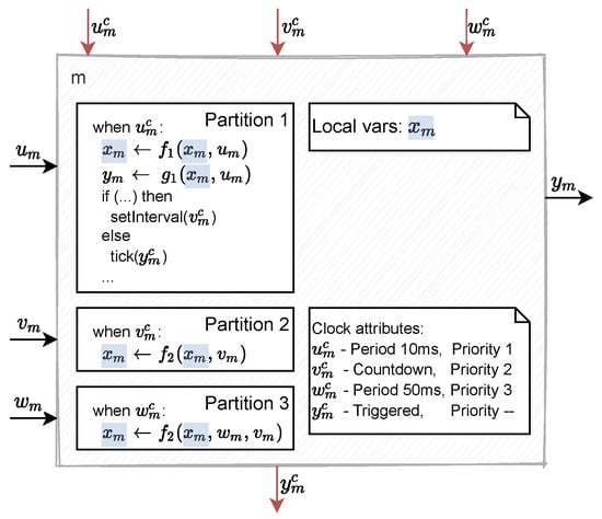
Figure 6.
Motivating example, where an FMU declares three input clocks (), one output clock , three input ports (), and one output port ().
A model partition, or just partition, represents code that should be executed when input clock ticks. Partitions contain arbitrary code that reads the inputs of the FMU, writes to the FMU’s local variables (which can be shared among tasks) and outputs, and potentially triggers output clocks or updates the interval of other input clocks. The inputs to each partition are set immediately before executing that partition as part of its corresponding task. In Figure 6, the input clock ’s partition reads and writes the shared variable , and either updates the interval of or activates/ticks the output clock .
We stress the distinction between a model partition and a task: the former represents code that is executed within the context of the latter. Therefore, a task T contains code that sets the inputs of the FMU, activates the model partition P, which indirectly activates an input clock, and reads the updated outputs. Such a task will be denoted as “P’s task”. For example, in Figure 6, when execution Partition 1’s task, the importer sets the values for input before executing the code of Partition 1.
In SE, there is a need for a function that the importer invokes, to tell the FMU to execute a partition, this function indirectly triggers the input clock of the partition. Consequently, the function is not used in SE. Nevertheless, the function is still used to inform the importer that a task should be scheduled.
In Figure 6, input clock ticks every 10ms and input clocks ticks every 50ms, so every so often, the two clocks will tick simultaneously. However, since tasks cannot run in parallel, the scheduler/importer must schedule the task sequentially according to their priority. As a result, the FMU must declare a priority level for each input clock using the attribute priority in the modelDescription file. In Figure 6, ’s task (the one executing Partition 1) should be executed before ’s (Partition 3), since the input clock has a higher priority than .
Output clocks, in SE, are never directly associated with a partition. Instead, these can be connected to input clocks (including the ones of the owning FMU) to indicate that a task should be scheduled.
Because tasks can be pre-empted, certain operations, such as updating a shared variable, must be atomic (see example below). As such, the FMU must inform the importer when it should not be interrupted to prevent mixed resource access that would create inconsistent values. The FMI standard provides a mechanism called locking and strongly encourage disjoint partitions to solve this problem.
Since partitions can trigger and update the interval of other clocks, there must be a mechanism for the FMU, in the middle of the calculation of a partition, to inform the importer that a clock has ticked or has a new interval, so that the importer can schedule the corresponding tasks. This information is in FMI communicated as a callback function.
Figure 7 illustrates a possible execution trace of the tasks corresponding to the partitions declared in Figure 6. At the initial wall-clock time , Task 1 and Task 3 are scheduled to execute. Since Task 1 has a higher priority, it runs first, and Task 3 is delayed. When executing Task 1, the FMU informs the importer that ’s task (Task 2) should be scheduled to run at wall-clock time . At wall-clock time , Task 1 is still executing, so Task 2 is delayed until wall-clock time since Task 1 has higher priority than Task 2. At , Task 2 starts executing (it has a higher priority than Task 3), but note that the activation time of Task 2 is still its original scheduled time . This is where the wall-clock time differs from the simulated time . At , Task 2 is pre-empted by Task 1. Finally, after being delayed substantially, Task 3 gets to execute, with its simulated time .
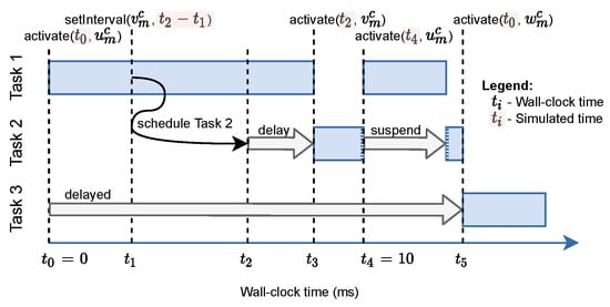
Figure 7.
Example execution trace of Figure 6.
It is the implementor’s responsibility of an SE FMU to ensure that all tasks are schedulable and can meet their deadlines. The importer only needs to ensure that the tasks are scheduled in the correct order.
4.2. Scheduled Execution Semantics
The following formalization is a simplification to highlight the main functions of the SE interface defined in the FMI standard. The main concepts being formalized are tasks, clocks, and activation of model partitions.
Definition 15 (SE FMU Instance).
An SE FMU instance with identifier m is represented by the tuple:
where:
- , , , , and , are defined as in Definition 1.
- and are functions to set the inputs and get the outputs, respectively. In contrast with the SC FMU in Definition 1, does not alter m’s state because any non-trivial computation of outputs should be done in the partitions associated with the input clocks, executed through the invocation of the function. Please note that we do not divide the variables into continuous and discrete variables in SE.
- queries the output clocks. Please note that in contrast to SC, changes the state of m, because it automatically de-activates (the justification is provided below). The clocks can again be either time-based or triggered.
- is a function representing the computation of a partition. If m is in state at wall-clock time t, represents three successive steps: the activation of the input clock , the computation of the partition associated with the input clock , and de-activation of clock . In the new state , clock is inactive. The returned variables b and denotes if the partition was pre-empted and the time it was pre-empted or completed.
- is the function that allows the importer to query the time of the next clock tick. It is defined as in Definition 1.
- is an injective function that determines the unique priority of each task. The priority of a task is fixed during the simulation.
- links a task/input clock with the set of variables (its partition) describing the input ports the task relies on and the output ports the task produces. It is strongly recommended that output and input variables are assigned uniquely to a model partition to avoid data inconsistencies. We assume that all inputs and outputs are a part of a partition ().
- links a task with a set of output clocks that can be activated by the task. We assume that all output clocks are a part such partition (), since they otherwise never would be activated by the FMU.
- links a task with a set of time-based input clocks. The set of input clocks denotes the clocks whose schedule may be affected by the computation of a specific partition.
The functions , , can be inferred from the modelDescription file of the FMU m. Please note that each task is triggered by the activation of an input clock, which is the reason for defining the functions , , , and in terms of the input clocks.
4.3. Composing SE FMUs
SE FMUs can as SC FMUs be coupled to form a scenario by connecting outputs of one FMU to inputs of another FMU.
Definition 16 (SE Scenario).
A scenario of SE FMUs is a structure where , L, and are defined as in Definition 2.
4.4. SE Semantics
We now present the semantics of the actions in Definition 15 to ensure a consistent interpretation. We start by introducing the run-time state of an SE FMU in Definition 17, which we modify using the actions described in Definition 15. The run-time state of an SE FMU differs from the run-time state of an SC FMU to be able to keep track of the current running partition. Furthermore, we can make some simplifications since the time of the SE is not superdense, meaning we do not need to keep track of the simulation mode of a given FMU.
Definition 17 (SE Run-time State).
Given an SE FMU m as defined in Definition 15, the run-time state of FMU m is a member of the set: , where:
- is an abstraction of the current time of the FMU m. The time is set by the importer to inform the FMU about the time on an event.
- , , and are defined in Definition 3.
- is a function linking each task/input clock with the last time its task was successful executed.
- denotes the input clock associated with the partition currently being computed in m. The notation denotes that the task/computation associated with the input clock is running. The notation furthermore means that the input clock is active. We use the notation to illustrate that no partition is being computed, which results in the absence of an associated input clock.
The semantics of the functions that appear in both the SE and SC interface are actually different not only because they operate on a different state space, but also because their semantics are different. For example, we need to include the aspect of preemptive tasks and model partitions in the SE semantics.
The importer stores such as in the SC simulations the schedule of the timed-based clocks in the function . The function links each time-based clock with the next time instance the clock should tick.
A task/partition that is scheduled to time , due to the priorities chosen and consequent delays incurred, may only execute at a later wall-clock time . We say that the model partition associated with the time-based input clock is schedulable or computable at the current time if . When is executed, it should set the relevant input ports () through the function , activate the partition through the function , and possibly read the calculated output ports (), through the function . Notice that we do not explicitly define the notion of a task in the formalization. Instead, we have an explicit notion of the computation of a partition ().
Definition 18 (Setting a Value at an Input Port).
An input port can be set to a value at a given time t using the action . The action is defined as follows:
where:
The precondition (above) states that an input port can be set if it has not yet been set (). Another requirement is that no partition is currently being computed that has a higher priority that the task associated with the input port.
The postcondition (below) states that the value of the input port is set and that the time of the input port is updated to the time of the assigned value.
Please note that the FMI standard forbids to call after an on the SE FMU m without an call in between. The standard also requires that the and functions are considerably faster than the function. We will therefore describe the semantics of the action next.
Definition 19 (Computing a Partition).
A partition of an input clock of an SE FMU at time t can be calculated at the simulated time using the action, :
where:
The precondition (above) requires that the partition associated with the input clock is not currently being computed () and the simulated time to active the clock is not in the future (). If the input clock is a time-based clock (), its schedule is checked to ensure that the partition is schedulable. If a partition is currently being computed (), we need to ensure that the computed partition is not locked and the priority of the currently computing partition is lower than the priority of the partition we want to compute () to ensure we do not interrupt a higher priority computation. To ensure that the partition can be computed using the correct input values, we require that all task inputs () must be set, such that they are defined at the simulated time of the event (set to a value at time ).
The postcondition (below) updates the time of the FMU to ; the timestamp where the partition computation was interrupted or done. The variable b denotes whether the task was interrupted or not. If the computation of the partition was not interrupted , we know that no partition is currently being executed and that the partition associated with is no longer schedulable/computable, which we ensure by setting its schedule to ∞. The timestamp of the input clock is updated to the time of the FMU to indicate that the partition of has been successfully computed. We also respect the lock of a task, ensuring that a locked task/partition cannot be interrupted. If the computation was interrupted , the computation of is still computable/schedulable, so we do not change the schedule of the task, since the computation must be resumed such that its outputs can be properly computed. An interruption also means that another partition is running ().
Unless otherwise stated by the FMU or importer, a partition/task can be pre-empted at any moment. To allow the FMU to inform its environment that the currently executing task () should not be pre-empted, FMI defines two functions: and that the FMU and importer can invoke. The function informs the environment that a task cannot be pre-empted until the function is invoked. We denote that a task is locked by the function , where if the task of cannot be pre-empted.
After a partition has been computed using the function, the computed output values can be obtained using the action , which is defined as follows:
Definition 20 (Obtaining a Value of an Output Port).
A value of an output variable of an SE FMU at time t is obtained by the action . The action is defined as follows:
where:
The precondition (above) states that the value of the output port has not been obtained since it was computed. We ensure this by requiring that the time of is less than the time of the input clock associated with the partition of . This means that the task computing the value of the output port has been computed at least once since the output port was last queried. Furthermore, we require no currently active task is updating the output port , formally . The last check can be ignored if all partitions are disjoint.
The postcondition (below) states that the value of the output port is obtained and that time of the output port is updated and that nothing else is changed.
- Scheduling Tasks
In SE, the importer operates as a scheduler of tasks to activate the model partitions according to a dynamic schedule. As summarized in Table 1, clocks can be ticked by the FMU or the importer. The FMU activates output clocks while the importer activates input clocks. Nevertheless, we focus on input clocks since these are the ones that are associated with a partition (when an output clock ticks, the importer is responsible for ticking all connected input clocks and scheduling the computation of the corresponding model partitions). Right after invoking on an output clock that is active, the clock should be inactive in state to ensure that the importer only schedules partitions/tasks that are associated with the output clock via a clocked connection once.
Since an input clock, may tick, the importer must be able to pre-empt the computation of partition to schedule a computation with a higher priority. Moreover, the schedule of certain time-based input clock can change during an computation. The importer, therefore, implements a function that an FMU can invoke (in the FMI standard, this is implemented as a callback mechanism) to signal that the status and interval of a time-based input clock has changed. The importer, inside , may consult these changes (through the functions and ), and schedule the corresponding tasks accordingly.
The time at which the importer schedules a given is computed according to: the input clock ’s declared interval; the function ; or through the function of some other output clock and FMU instance connected to the input clock . In the last case, is scheduled to execute as soon as possible, according to the priorities known to the importer.
Definition 21 (Getting the State of an Output Clock).
Getting the state of the output clock of an SE FMU at time t using the action, changes the state of the FMU according to:
where:
The precondition (above) requires that the output clock has not been queried since it was computed as a part of an active task. We ensure this by requiring that at least one of the input clocks () associated with a task that can tick the output clock has been activated since the last time the output clock was queried.
The postcondition (below) updates the timestamp of the output clock . It also makes the output clock inactive, which is required to ensure that the importer only schedules tasks that are associated with the output clock via a clocked connection one time.
Since the computation of a partition can change the interval of a time-based input clock the importer must be able to dynamically obtain the interval of a time-based input clock through the function . The function is known as a part of callback triggered by the FMU to inform the importer that the interval of an input clock has changed. Please note that the callback function is known as part of the computation of a partition, so it is not necessary to invoke the function explicitly. The function is defined next.
Definition 22 (Scheduling a task).
The action retrieves the interval to the next tick of the clock . The action is defined as:
where:
The precondition (above) states that the interval of the input clock should be unknown (denoted in our semantics by ∞) or that it should be the case that the interval of the input clock might have been changed by the current running task.
The postcondition (below) updates the schedule of the input clock to reflect the next event of the clock. If the function returns , meaning that the task of the input clock has no current schedule, we set its schedule to .
- Generic Scheduled Execution Algorithm
We have now described the primary actions of an SE FMU. The following paragraph will shortly describe how these actions can be composed to form an orchestration algorithm used to simulate an SE scenario defined in Definition 16.
Let denote a set of FMU instances, assumed to be initialized.
- 1.
- Schedule , for all and all , if interval of is constant, fixed, or calculated;
- 2.
- When is invoked, do:
- (a)
- Lock pre-emption with ;
- (b)
- If , schedule for any clock that is transitively connected to .
- (c)
- For all
- i.
- ii.
- If , then schedule the task for clock at time t.
- (d)
- Unlock pre-emption with ;
- 3.
- Each task is implemented as:
- (a)
- Set the inputs of m using (locking pre-emption with and if needed);
- (b)
- Invoke , where is the simulated time that was scheduled to execute.
- (c)
- Get the outputs of m using (locking pre-emption with and if needed);
5. Related Work
Synchronous clocks are one of the solutions proposed to tackle the more general challenge of co-simulating hybrid systems. Other proposals have been made in the state of the art, but none of them tackle the problem of discerning different simultaneous events in the context of co-simulation. For instance, ref. [25] proposes a master algorithm for hybrid co-simulation. The proposal includes support for absent signals, mandatory implementation of rollback, zero duration step size, co-simulation FMUs supporting feedthrough, and predictable step sizes. However, it excludes algebraic loops, due to the introduced non-determinism. Our proposed interfaces enable algebraic loop resolution, even when clocks are involved, but does not provide guarantees of convergence.
An extensive study of hybrid system simulation challenges was carried out in [26], and includes, for example, the possibility of an event iteration driving the system into chattering. And [27,28,29] focus such discussion in the context of the FMI standard, providing solutions to some of these challenges. These works complement ours by helping importers assess whether a given simulation scenario is well behaved. We refer the reader to [17] for more references in co-simulation of hybrid systems.
The goal of this paper is to describe the main mechanisms standardized in the FMI standard that enable synchronous clocked simulation and scheduled execution. We can therefore highlight related work that share the same goals.
Regarding SC simulation, we highlight the work in [30,31] that introduces the synchronous clocks constructs used in the Modelica language, specified in [5]. Such work, and references thereof on synchronous languages [13,32], were used as basis for the definition of the SC approach described here. The main difference is that an SC clock does not enforce a partition on the equations that can be written by it. These differences make it more difficult to ensure well-formedness of co-simulation scenarios, but provide more flexibility, reflecting the heterogeneous use cases of FMI.
In the domain of scheduled execution, we highlight the OSEK/VDX [33] and AUTOSAR standards, which enable different suppliers to develop and test software independently, and subsequently integrated the different applications. Such work complements the SE interface by standardizing the importer environment, where FMU SE instances can execute.
Formal semantics of the FMI 1.0 and FMI 2.0 have previously been studied in [23,34]. Cavalcanti et al. [34] claim to provide the first behavioral semantics of FMI 1.0. The operational semantics of FMI 2.0 has been studied in [23,35]. Our work extends previous work by treating the FMI 3.0 standard, which is a superset of the previous FMI standards.
6. Conclusions
This paper summarizes the results of the FMI project developing black-box simulation units with synchronous clocks to provide a suitable event mechanism for simulating continuous systems with an event-driven nature in the FMI universe. The Modelica language inspired the introduction of synchronous clocks into the FMI standard. The paper presents formal semantics for two new interfaces of the FMI 3.0 standard to ensure a precise and unambiguous conceptualization of the new interfaces that can serve as a basis for implementing the supporting tools to ensure a continued industrial adaption of the new version of the FMI standard. The semantics also strives towards a more unified understanding of well-formed scenarios and FMI-based simulations, which will be studied in future work. Future work also includes the development of concrete tools based on sound approaches for synthesizing orchestration algorithms, which will enable co-simulation practitioners to use formal methods in the secret ninja style enabling practitioners to leverage recent advantages of modern SMT-solvers to verify their use of the FMI standard.
Limitations
Despite the paper’s focus on precision, the FMI standard document continuously improves and therefore remains the source of truth. We refer the reader to [36] for an account of essential features developed for the FMI 3.0 standard. Regarding the limitations of the interface itself, it is intentional that the orchestration algorithm is underspecified, as it not part of the standardization efforts. Continued work focuses on designing valid orchestration algorithms, which usually constitute intellectual property for the companies supporting the FMI interface.
Author Contributions
Thearticle was structured and mainly written by S.T.H. and C.Â.G.G. but resulted from close collaboration between all the authors. The scheduled execution material was prepared with M.B. and I.Z. The material on synchronous clocks was prepared together with O.K., A.J., T.S., P.R.M., K.S., K.W., C.B. and T.B. M.N. has provided continuous support for the structure and content of the article. All authors have read and agreed to the published version of the manuscript.
Funding
This research received no external funding.
Data Availability Statement
Not applicable.
Acknowledgments
Simon Thrane and Cláudio Gomes are grateful to the Poul Due Jensen Foundation, which has supported establishing a new Centre for Digital Twin Technology at Aarhus University. Furthermore, we would like to thank the following people for their input and support: Stefan Hallerstede, Peter Gorm Larsen, and Jaco van de Pol. Finally, we are thankful to the Modelica association for its continued support of the FMI Project.
Conflicts of Interest
The authors declare no conflict of interest.
Abbreviations
The following abbreviations are used in this manuscript:
| FMI | Functional Mock-up Interface |
| FMU | Functional Mock-up Unit |
| SC | Synchronous clocks |
| SE | Scheduled Execution |
| ME | Model Exchange |
| CS | Co-simulation |
| Inputs | |
| Outputs | |
| Input clocks | |
| Output clocks | |
| F | Feedthrough |
| The set of FMUs that may prematurely terminate a step | |
| L | Coupling |
| Clock Coupling |
References
- Cremona, F.; Lohstroh, M.; Tripakis, S.; Brooks, C.; Lee, E.A. FIDE. In Proceedings of the 31st Annual ACM Symposium on Applied Computing, Pisa, Italy, 4–8 April 2016. [Google Scholar] [CrossRef]
- Paris, T.; Wiart, J.; Netter, D.; Chevrier, V. Teaching co-simulation basics through practice. In Proceedings of the SummerSim’19, Berlin, Germany, 22–24 July 2019; Durak, U., Ed.; ACM: New York, NY, USA, 2019. [Google Scholar]
- 2.0, F. Functional Mock-up Interface for Model Exchange and Co-Simulation. Available online: https://fmi-standard.org/downloads/ (accessed on 30 October 2022).
- FMI. Functional Mock-up Interface Tools. Available online: https://fmi-standard.org/tools/ (accessed on 30 October 2022).
- Modelica Association. Modelica—A Unified Object-Oriented Language for Systems Modeling. Available online: https://modelica.org/documents/MLS.pdf (accessed on 30 October 2022).
- Dahmann, J.S. High Level Architecture for Simulation. In Proceedings of the DIS-RT, Eilat, Israel, 9–10 January 1997; pp. 9–14. [Google Scholar]
- Tendeloo, Y.V.; Vangheluwe, H. Discrete Event System Specification Modeling and simulation. In Proceedings of the WSC, Gothenburg, Sweden, 9–12 December 2018; pp. 162–176. [Google Scholar]
- Zeigler, B.P. Theory of Modeling and Simulation; John Wiley: Hoboken, NJ, USA, 1976. [Google Scholar]
- Awais, M.U.; Mueller, W.; Elsheikh, A.; Palensky, P.; Widl, E. Using the HLA for Distributed Continuous Simulations. In Proceedings of the 2013 8th EUROSIM Congress on Modelling and Simulation, Cardiff, Wales, UK, 10–13 September 2013; pp. 544–549. [Google Scholar] [CrossRef]
- Awais, M.U.; Palensky, P.; Elsheikh, A.; Widl, E.; Stifter, M. The high level architecture RTI as a master to the functional mock-up interface components. In Proceedings of the ICNC, San Diego, CA, USA, 28–31 January 2013; pp. 315–320. [Google Scholar]
- Zacharewicz, G.; Giambiasi, N.; Frydman, C.S. GDEVS/HLA Environment: A Time Management Improvement. In Proceedings of the 17th IMACS World Congress on Scientific Computation, Applied Mathematics and Simulation, Paris, France, 11–15 July 2005. [Google Scholar]
- Yilmaz, F.; Durak, U.; Taylan, K.; Oğuztüzün, H. Adapting Functional Mockup Units for HLA-compliant Distributed Simulation. In Proceedings of the 10th International Modelica Conference, Lund, Sweden, 10–12 March 2014; pp. 247–257. [Google Scholar] [CrossRef]
- Benveniste, A.; Caspi, P.; Edwards, S.; Halbwachs, N.; Le Guernic, P.; de Simone, R. The Synchronous Languages 12 Years Later. Proc. IEEE 2003, 91, 64–83. [Google Scholar] [CrossRef]
- Kübler, R.; Schiehlen, W. Two Methods of Simulator Coupling. Math. Comput. Model. Dyn. Syst. 2000, 6, 93–113. [Google Scholar] [CrossRef]
- 3.0, F. Functional Mock-Up Interface for Model Exchange, Co-Simulation, and Scheduled Execution. Available online: https://fmi-standard.org/downloads/ (accessed on 15 May 2022).
- Gomes, C.; Najafi, M.; Sommer, T.; Blesken, M.; Zacharias, I.; Kotte, O.; Mai, P.R.; Schuch, K.; Wernersson, K.; Bertsch, C.; et al. The FMI 3.0 Standard Interface for Clocked and Scheduled Simulations. In Proceedings of the 14th International Modelica Conference, Linköping, Sweden, 20–24 September 2021; Sjölund, M., Buffoni, L., Pop, A., Ochel, L., Eds.; Modelica Association and Linköping University Electronic Press: Linköping, Sweden, 2021. Number 181 in Linköping Electronic Conference Proceedings. [Google Scholar] [CrossRef]
- Gomes, C.; Thule, C.; Broman, D.; Larsen, P.G.; Vangheluwe, H. Co-Simulation: A Survey. Acm Comput. Surv. 2018, 51, 1–33. [Google Scholar] [CrossRef]
- Lee, E.A.; Zheng, H. Operational Semantics of Hybrid Systems. In Hybrid Systems: Computation and Control; LNCS; Springer: Berlin/Heidelberg, Germany, 2005; Volume 3414. [Google Scholar] [CrossRef]
- Hansen, S.T.; Gomes, C.; Larsen, P.G.; van de Pol, J. Synthesizing Co-Simulation Algorithms with Step Negotiation and Algebraic Loop Handling. In Proceedings of the Annual Modeling and Simulation Conference (ANNSIM’21), Virtual, 28 January 2021; Martin, C.R., Blas, M.J., Inostrosa-Psijas, A., Eds.; IEEE: Piscataway, NJ, USA, 2021. [Google Scholar]
- Tarjan, R. Depth-First Search and Linear Graph Algorithms. In Proceedings of the 12th Annual Symposium on Switching and Automata Theory (Swat 1971), East Lansing, MI, USA, 13–15 October 1972; Volume 1. [Google Scholar] [CrossRef]
- Abrial, J.R. Modeling in Event-B—System and Software Engineering; Cambridge University Press: Cambridge, UK, 2010. [Google Scholar]
- Fitzgerald, J.; Fitzgerald, J.S. Validated Designs for Object-Oriented Systems; Springer: London, UK, 2005. [Google Scholar]
- Hansen, S.T.; Gomes, C.; Palmieri, M.; Thule, C.; van de Pol, J.; Woodcock, J. Verification of Co-simulation Algorithms Subject to Algebraic Loops and Adaptive Steps. In Proceedings of the FMICS’21, Paris, France, 24–26 August 2021; Lluch Lafuente, A., Mavridou, A., Eds.; LNCS. Springer: Cham, Switzerland, 2021; Volume 12863. [Google Scholar]
- Broman, D.; Brooks, C.X.; Greenberg, L.; Lee, E.A.; Masin, M.; Tripakis, S.; Wetter, M. Determinate composition of FMUs for co-simulation. In Proceedings of the EMSOFT’13, Montreal, QC, Canada, 29 September–4 October 2013; Ernst, R., Sokolsky, O., Eds.; IEEE: Piscataway, NJ, USA, 2013. [Google Scholar]
- Cremona, F.; Lohstroh, M.; Broman, D.; Di Natale, M.; Lee, E.A.; Tripakis, S. Step Revision in Hybrid Co-Simulation with FMI. In Proceedings of the 14th ACM-IEEE International Conference on Formal Methods and Models for System Design, Kanpur, India, 18–20 November 2016. [Google Scholar]
- Mosterman, P.J.; Biswas, G. A Comprehensive Methodology for Building Hybrid Models of Physical Systems. Artif. Intell. 2000, 121, 171–209. [Google Scholar] [CrossRef]
- Tripakis, S. Bridging the semantic gap between heterogeneous modeling formalisms and FMI. In Proceedings of the 2015 International Conference on Embedded Computer Systems: Architectures, Modeling, and Simulation, SAMOS 2015, Samos, Greece, 19–23 July 2015; Soudris, D., Carro, L., Eds.; IEEE: Piscataway, NJ, USA, 2015. [Google Scholar] [CrossRef]
- Broman, D.; Greenberg, L.; Lee, E.A.; Masin, M.; Tripakis, S.; Wetter, M. Requirements for Hybrid Cosimulation Standards. In Proceedings of the 18th International Conference on Hybrid Systems: Computation and Control, HSCC ’15, Seattle, WA, USA, 14–16 April 2015; ACM: New York, NY, USA, 2015. [Google Scholar] [CrossRef]
- Liboni, G.; Deantoni, J.; Portaluri, A.; Quaglia, D.; De Simone, R. Beyond Time-Triggered Co-Simulation of Cyber-Physical Systems for Performance and Accuracy Improvements. In Proceedings of the 10th Workshop on Rapid Simulation and Performance Evaluation: Methods and Tools, Manchester, UK, 22–24 January 2018. [Google Scholar]
- Otter, M.; Thiele, B.; Elmqvist, H. A Library for Synchronous Control Systems in Modelica. In Proceedings of the 9th International Modelica Conference, Munich, Germany, 3–5 September 2012. [Google Scholar] [CrossRef]
- Elmqvist, H.; Otter, M.; Mattsson, S.E. Fundamentals of Synchronous Control in Modelica. In Proceedings of the 9th International Modelica Conference, Munich, Germany, 3–5 September 2012. [Google Scholar] [CrossRef]
- Colaço, J.L.; Pouzet, M. Clocks as First Class Abstract Types. In Embedded Software; LNCS; Alur, R., Lee, I., Eds.; Springer: Berlin/Heidelberg, Germany, 2003; Volume 2855. [Google Scholar] [CrossRef]
- ISO 17356-3:2005; Road Vehicles—Open Interface for Embedded Automotive Applications—Part 3: OSEK/VDX Operating System (OS). Available online: https://www.iso.org/standard/40079.html (accessed on 15 December 2020).
- Cavalcanti, A.; Woodcock, J.; Amálio, N. Behavioural Models for FMI Co-simulations. In Proceedings of the ICTAC’16, Taipei, Taiwan, 24–31 October 2016; LNCS. Sampaio, A., Wang, F., Eds.; Springer: Cham, Switzerland, 2016; Volume 9965. [Google Scholar]
- Gomes, C.; Lucio, L.; Vangheluwe, H. Semantics of Co-Simulation Algorithms with Simulator Contracts. In Proceedings of the ACM/IEEE MODELS’19, Munich, Germany, 15–20 September 2019; Burgueño, L., Pretschner, A., Voss, S., Chaudron, M., Kienzle, J., Völter, M., Gérard, S., Zahedi, M., Bousse, E., Rensink, A., et al., Eds.; IEEE: Piscataway, NJ, USA, 2019. [Google Scholar]
- Junghanns, C.; Blochwitz, T.; Bertsch, C.; Sommer, T.; Wernersson, K.; Pillekeit, A.; Zacharias, I.; Blesken, M.; Mai, P.; Schuch, K.; et al. The Functional Mock-up Interface 3.0-New Features Enabling New Applications. In Proceedings of the 14th International Modelica Conference, Online, 20–24 September 2021; Linköping University Electronic Press, Linköpings Universitet: Linköping, Sweden, 2021. [Google Scholar]
Publisher’s Note: MDPI stays neutral with regard to jurisdictional claims in published maps and institutional affiliations. |
© 2022 by the authors. Licensee MDPI, Basel, Switzerland. This article is an open access article distributed under the terms and conditions of the Creative Commons Attribution (CC BY) license (https://creativecommons.org/licenses/by/4.0/).