
Optimal Field Sampling of Arc Sources via Asymptotic Study of the Radiation Operator


Dipartimento di Ingegneria, Università della Campania “Lugi Vanvitelli”, Via Roma 29, 81031 Aversa, Italy
*
Author to whom correspondence should be addressed.
Electronics 2022, 11(2), 270; https://doi.org/10.3390/electronics11020270
Submission received: 13 December 2021
/
Revised: 7 January 2022
/
Accepted: 11 January 2022
/
Published: 14 January 2022
(This article belongs to the Topic Antennas)
Abstract
:In this paper, the question of how to efficiently sample the field radiated by a circumference arc source is addressed. Classical sampling strategies require the acquisition of a redundant number of field measurements that can make the acquisition time prohibitive. For such reason, the paper aims at finding the minimum number of basis functions representing the radiated field with good accuracy and at providing an interpolation formula of the radiated field that exploits a non-redundant number of field samples. To achieve the first task, the number of relevant singular values of the radiation operator is computed by exploiting a weighted adjoint operator. In particular, the kernel of the related eigenvalue problem is first evaluated asymptotically; then, a warping transformation and a proper choice of the weight function are employed to recast such a kernel as a convolution and bandlimited function of sinc type. Finally, the number of significant singular values of the radiation operator is found by invoking the Slepian–Pollak results. The second task is achieved by exploiting a Shannon sampling expansion of the reduced field. The analysis is developed for both the far and the near fields radiated by a 2D scalar arc source observed on a circumference arc.
1. Introduction
The question of sampling the field radiated by a source or the one scattered by an object is a classical research topic of the electromagnetics literature [1,2,3,4,5,6,7,8,9].
On one hand, a proper sampling of the radiated/scattered field allows representing the field from the knowledge of its samples in a discrete and finite number of points. On the other, it allows acquiring independent information to address the correspondent inverse source/inverse scattering problem [10,11].
In this paper, the attention is limited to the sampling of the radiated field which is linked to the source current by a linear operator called radiation operator.
1.1. Literature Review
Classical sampling schemes of the radiated field for the case of planar [12], cylindrical [13] and spherical scanning [14] were proposed. Despite this, such schemes do not take into account explicitly the source shape; for such reason, they require collecting a number of field measurements that may be significantly higher than the number of degrees of freedom (NDF) of the radiated field [15,16]. The latter represents the number of independent parameters required to represent the radiated field with good accuracy and, at the same time, the minimum number of field measurements required to reconstruct the source current stably.
The acquisition of a number of field samples larger than the number of degrees of freedom affects badly the acquisition time and also the processing time to interpolate the field samples or to retrieve the source current. For such a reason, it is of great interest to devise a sampling scheme that exploits a non-redundant number of field measurements.
To reduce the number of measurements, over the years different sampling schemes have been proposed. A first strategy is based on an adaptive procedure that increases the sampling rate only when the measured field oscillates faster [17]. In [18], an efficient sampling scheme suitable for any source enclosed in an ellipsoid is devised by exploiting reasoning on the local bandwidth of the reduced field. Such a sampling scheme can be used also for the planar disk and spherical sources that can be seen as particular cases of the ellipsoidal source.
Recently, a new method that exploits the point spread function (PSF) in the observation domain has been proposed in [19]. Such a method relies on the idea that two adjacent points are independent if the main lobes of the centered in such points do not overlap and, hence, are distinguishable from each other.
Other methods recast the question of efficiently sampling the radiated field as a sensor selection problem and choose the optimal sampling points in such a way that the radiation operator and its discrete counterpart exhibit the same relevant singular values. Such a goal can be achieved by exploiting a numerical procedure that optimizes a metric related to the singular values [20,21,22] or, alternatively, by an analytical study and a proper discretization of the radiation operator [23,24,25].
1.2. Goal of the Paper
Here, with reference to a 2D geometry consisting of a circumference arc source whose radiated field is collected on a circumference observation arc, the minimum number of measurements required to discretize the radiated field without loss of information is first determined. From the mathematical point of view, this implies an evaluation of the NDF of the source over the assigned observation domain. This task is performed by computing analytically the number of relevant singular values of the radiation operator with the asymptotic approach proposed in [25]. Next, an efficient interpolation formula of the radiated field is found by exploiting a sampling representation of the left singular functions of the radiation operator.
Let us remark that the optimal locations of the sampling points and an efficient interpolation formula of the field radiated by a circumference arc source are provided also in [19] by a numerical procedure. Here, instead, the optimal sampling points and the basis functions used in the interpolation stage of the radiated field are analytically found. This allows highlighting the key role played by the geometric parameters of the problem.
The paper is organized as follows. In Section 2, the geometry of the problem and the explicit expression of the radiation operator in the case of an observation domain in far-field and near-field is provided. In Section 3, an outline of our sampling strategy is shown. In Section 4, the NDF and an efficient interpolation formulation of the far field are derived. In Section 5, all the results of Section 4 are extended to the case of an observation domain in near field. In Section 6, for sake of comparison, a sampling scheme based on a uniform sampling step is considered and the number of measurements points saved by our non-uniform sampling scheme with respect to the uniform case is estimated. In Section 7, a numerical validation of our analytical results on the NDF and the field sampling is shown. Conclusions follow in Section 8.
2. Geometry of the Problem
Consider the 2D scalar geometry depicted in Figure 1 where the y-axis represents the direction of invariance. An electric current is supported over an arc of circumference of radius spanning the interval .
The electric field radiated by such source is observed on an arc of circumference of radius that subtends an angular sector .
For the considered geometry, the radiation operator is defined as
where and denotes the set of square integrable functions on and , respectively. Apart some unessential factors, such operator can be explicitly written as
where the 2D Green function is given by
with
Since the radiation operator is linear and compact, its singular values decomposition can be introduced. The latter is provided by the triple where the right singular functions and the left singular functions represent a set of basis functions for the density current and the radiated field , instead, stand for the singular values. As well known, the right and the left singular functions are related by the following equations
where stands for the adjoint operator. Hereafter, the adjoint operator is not defined as usual since a weight function is introduced in its definition. In other words, is defined as
with denoting the conjugate of the Green function.
It is worth noting that the use of a weighted adjoint affects only the shape of the singular values behavior of but not the critical index after which they abrupt decay. For such reason, it can be used to estimate the most significant singular values of the radiation operator.
3. Outline of the Sampling Strategy
In this section, the methodology followed in the paper is described and an outline of such methodology is sketched in the block diagram of Figure 2.
The first aim of the paper is to provide a closed form expression of the NDF of the radiated field. The NDF is estimated by evaluating the number of relevant singular values of the radiation operator. In particular, since the eigenvalues of the auxiliary operator are the square of the singular values of , the number of relevant singular values of the radiation operator will be evaluated by studying the eigenvalue problem . The latter can be explicitly written as
where the kernel is given by
Here, such a kernel is estimated by exploiting an asymptotic approach. After, by exploiting a change of variables and proper choice of the weight function, such a kernel is recast like a sinc kernel of convolution type multiplied by a phase exponential. Finally, by redefining the eigenfunctions, the eigenvalues problem is rewritten in a new form with a purely sinc kernel. This allows exploiting the Slepian–Pollak theory to estimate the number of relevant eigenvalues of which, as said before, provides an estimation of NDF of the radiated field.
The second aim of the paper is to provide the optimal sampling where the field must be collected and an interpolation formula of the radiated field that exploits a non-redundant number of field samples. To achieve this goal, the Shannon sampling theorem is adopted to derive a sampling representation of the reduced field in the warped variable. Then, starting from it, an efficient interpolation formula of the radiated field is easily obtained.
The study is developed not only for an observation arc in far-field but also for a near-field configuration.
4. Optimal Sampling of the Far-Field
In this section, all the steps illustrated in Figure 2 are detailed to compute the NDF of the far-field and to provide an interpolation formula that exploits a non-redundant number of field samples.
4.1. Asymptotic Study of the Operator in Far Zone
I. The kernel of the auxiliary operator is particularized to the far-zone by substituting in (8) the far zone Green function. It follows that
with
For , the value of the kernel can be easily obtained by evaluating the integral .
For , the integral in (9) can be asymptotically evaluated if the condition is satisfied. The choice of the asymptotic technique is related to the presence/absence of stationary points in the phase function . In Appendix A, it is shown that if the following condition holds
then no stationary points fall into the set . In such a case, the kernel in (9) can be asymptotically evaluated by considering only the contribution by the endpoints and [26]. Accordingly, for each it results that
where denotes the partial derivative of with respect to hence, .
II. The kernel of in the variables is not convolution and this does not allow to find easily its eigenvalues. To make more similar to a convolution operator, it is first recast as
Then, the following variables
are introduced. Equations (14) and (15) allow rewriting the kernel of as
III. At this juncture, the kernel function has still an intricate structure. However, by expanding with respect to the variable in a Taylor series stopped at the first order, one obtains
Hence, taking into account of Equations (17) and (18), the kernel can be approximated as
IV. Now, the weight function must be chosen. The best choice for is to fix it in such a way that the eigenvalues of are known in closed form. Such goal can be reached by choosing
Then, the kernel can be recast as
where . Accordingly, in the variables , the eigenvalue problem can be expressed as
Let us note that the functions and introduced in (14) and (15) can be respectively rewritten as and . Such variables, apart for a scalar factor, are equal to the variables
commonly used in the study of far field problems. In the variables , the eigenvalue problem (23) becomes
V. To evaluate the eigenvalues of , let us fix
Then, the eigenvalue problem (24) can be recast in the simple and nice form
4.2. NDF Evaluation and Interpolation of the Far Field
VI. In the seminal work of Slepian and Pollak [27], the eigenvalues of Equation (26) have been deeply investigated. In particular, it has been shown that they exhibit a step-like behavior with the knee occurring at the index
where [] stands for the integer part. Such a number provides the number of relevant singular values of the radiation operator; hence, it can be taken as an estimation of the NDF of the far-field. Accordingly, N is also the minimum number of basis functions required to represent the far field with good accuracy. It is worth remarking that, when condition (11) is satisfied, the NDF of the far field radiated by a circumference arc source is exactly equal to that of the far field radiated by a strip source sharing the same endpoints of the arc.
VII. Once the minimum number of field samples has been established, let us provide an interpolation formula of the radiated field. To this end, it is worth nothing that the set of basis functions are bandlimited functions with a bandwidth . Accordingly, for each can be expressed through the following truncated sampling series [28]
where
- ;
- is the set containing all those indexes such that .
The set of functions represent a basis for the reduced field which is defined as
Accordingly, also the reduced field can be expressed through the truncated sampling series
VIII. Taking in mind of (29) and (30), it results that the far field can be written as
from which follows that
The latter represents an interpolation formula of the far field based on the Shannon sampling series of the reduced field. It is worth noting that the number of sampling points falling into the interval (or ) can be easily computed by the equation
Such a number is called Shannon number and it is essentially equal to the NDF of the far field. This means that the interpolation Formula (33) exploits a non-redundant number of field samples. Moreover, from Equation (33), it is evident that the optimal sampling points of the far field in the variable are given by
Hence, in the variable the optimal sampling points satisfy the equation
Accordingly, since the transformation is nonlinear, the uniform sampling in the variable is mapped into a non-uniform sampling in the variable .
5. Optimal Sampling of the near Field
In this section, all the steps shown in Figure 2 are repeated to evaluate the NDF and to provide an efficient interpolation formula of the near field.
5.1. Asymptotic Study of the of the Operator in Near Zone
I. To study the kernel of in near zone, let us rewrite it in a more explicit form by substituting the near zone Green function in (8). From this substitution, the following integral comes out
In order to evaluate such integral, let us fix
- ,
- .
Then, (36) can be rewritten as
At , the kernel of can be evaluated by computing the integral .
For , if the hypothesis is fulfilled, the integral (37) can be asymptotically evaluated. To establish if stationary phase points appear in the phase function, the equation must be solved for . The latter can be explicitly written as
Unfortunately, the previous equation cannot be analytically solved. For such reason, here, the attention is limited to all those cases where the geometrical parameters are such that no stationary points appear in the set . In particular, through a numerical analysis, it has been shown that
- fixing the source angle , the interval for which no stationary points appear on the source increases with the ratio .
- fixing the ratio , the interval for which no stationary points appear on the source decreases with the source angle .
This behavior can be observed in the tables of the Appendix B. From such tables, it is evident that in near zone the condition for the lack of stationary points in is given by
where is a function depending on the ratio whose values are reported in Table 1.
Accordingly, is a monotonic function and its diagram is shown in Figure 3.
For all the configurations in which no stationary points appear in the phase function , the integral in (37) can be evaluated by considering only the contributions by the endpoints. Then, it results that for each
II. In order to recast the kernel in a form more similar to a known convolution kernel, let us rewrite it as
Then, let us introduce the following functions
which allow recasting the kernel as
III. The kernel function (44) has still an intricate structure. However, if the numerator and the denominator of amplitude term are expanded with respect to the variable in a Taylor series truncated to the first order, the amplitude term can be simplified as below
IV. At this juncture, if the weight function is chosen as
the kernel can be recast as
Accordingly, in the variable the eigenvalues problem in (8) can be expressed as
from which follows that
V. Now, by fixing
the eigenvalues problem (49) can be rewritten in the simple and nice form
5.2. NDF Estimation and Interpolation of the near Field
VI. The eigenvalues of (51) can be found by resorting again to [27]. Accordingly, it is possible to state that the eigenvalues of (51) exhibit a step-like behavior with the knee occurring at the index
This number provides an estimation of the NDF of the near-field. Let us highlight that, when no stationary points appear in the integral (38), the NDF of the far-field radiated by a circumference arc source has the same mathematical expression of that of the near-field radiated by a strip source (see Equation (25) in [21]).
VII. At this juncture an interpolation formula of the near-field is provided. Since the set of basis functions are bandlimited functions with a bandwidth , for each can be expressed through the following truncated sampling series
where
- ;
- is the set containing all those index such that .
The set of functions represent a basis for the reduced field
Accordingly, it can be expressed by the following truncated sampling expansion
VIII. At this juncture, taking into account of (54) and (55), the near field can be approximated as below
Since , Equation (56) can be rewritten as
the previous equation provides an interpolation formula of the near field based on a Shannon sampling series of the reduced field. The number of field samples used by (57) is equal to the Shannon number which is given by
accordingly, also in the case of observation domain in near field, the Shannon number is exactly equal to the NDF. From Equation (57), it can be noted that the optimal locations of the sampling points in the variable are given by
hence, in the variable the optimal sampling points of the near-field can be found by solving numerically the equation
naturally, since the transformation is nonlinear, the uniform sampling in the variable is mapped into a non-uniform sampling in the variable . In particular, the optimal field samples are denser for small values of whereas their step is larger when approaches to .
6. Comparison between Non-Uniform and Uniform Sampling
In the previous section, a non-uniform sampling scheme for the far field and the near field has been shown. Here, for sake of comparison, a more standard sampling scheme based on a uniform sampling is recalled from the literature. It is well known that the field radiated by a source enclosed in a circle of radius can be expressed in a series of Fourier harmonics or periodic Dirichlet functions. In particular, if the observation domain is a full circumference (), the number of terms of such series can be truncated to where [] stands for the integer part of [29]. Instead, if the radiated field is observed on a limited angular interval , a number of terms
is sufficient to represent the radiated field with good accuracy [10].
Accordingly, if the observation domain is a limited arc extending on the angular sector , the field radiated by a source enclosed in a circle of radius can be expressed as below
where
- is the Dirichlet function
- are the sampling points uniformly spaced over the observation arc, hence, with and .
Now, it is possible to quantify the percentual reduction of field samples of the present non-uniform sampling scheme when it is compared with the uniform sampling strategies. The latter is given by
Accordingly, it results that the percentual reduction of field samples for the far-field and the near field can be approximated as below
7. Numerical Validation
In this section, the NDF evaluation and the interpolation formula of the radiated field provided in Section 4 and Section 5 are validated by a numerical analysis. Moreover, the non-uniform sampling strategies developed for the far field and the near field are compared with the uniform sampling strategies described in Section 6. In such comparison, the misfit between the exact field and its approximation provided by the interpolation is measured by the relative error
with denoting the Euclidean norm. In all the cases, the exact field will be that provided by Equation (2) while the interpolated field will be provided by (32), (57) or (62), according to the type of considered sampling (either non-uniform or uniform).
The numerical validation of the analytical results is provided in two subsections: the first concerning the far field sampling, the second one regarding the near-field sampling.
7.1. Far-Field Sampling Validation
In this section, a numerical check of the analytical results for the far field is provided. A circumference arc source of radius spanning the interval is considered. The density current of the source is chosen as
where . As is well known, such current radiates an electric field focusing at . The far field is observed on a circumference arc spanning the interval .
In Figure 4, the actual singular values of the radiation operator are compared with the ones obtained by considering the weighted adjoint.
As it is clear from Figure 4, the use of a weighted adjoint changes the behavior of the singular values but not the index at which they decay abruptly. The latter is predicted by (27) which, in the considered test case, returns in perfect agreement with the diagrams in Figure 4. In Figure 5, the optimal sampling points of the far-field in the variable are shown. They are non-uniformly arranged along the observation domain. In particular, the sampling step is minimum around the direction , whereas it increases by moving towards the directions .
In Figure 5, the exact far-field computed by means of the equation is compared with the field returned by the interpolation Formula (32).
As can be seen from Figure 6, despite the interpolation Formula (32) exploits a number of samples that is as low as possible (only non-uniform field samples are used for the interpolation), the interpolated field agrees very well with the exact field and 0.028.
In order to highlight the better performance of the non-uniform sampling with respect to the uniform one, in Figure 7 also the far field obtained by the interpolation of uniform samples is sketched. In particular, the blue line shows the field interpolated starting from uniform field samples while the green dashed one shows the one obtained from samples.
As can be seen from Figure 7, uniform field samples are not sufficient to approximate the exact far field and 0.814. On the contrary, uniform field samples allow to approximate well the exact far field with a relative error 0.029. From this numerical test, it is evident that only the non-uniform sampling scheme allows to achieve a good accuracy by employing a number of field samples equal to the NDF. The uniform sampling scheme can achieve the same accuracy as the non-uniform strategy, but it requires a larger number of field samples. In the considered example, the use of the non-uniform sampling strategy allows a reduction of the field measurements .
7.2. Near-Field Sampling Validation
In this section, some numerical experiments related to the analytical results for the near-field are sketched. A circumference arc source with and is considered. The source current is chosen as in (66) with . The radiated field is observed on a circumference arc with and . With reference to such a configuration, in Figure 8 the actual singular values of the radiation operator are compared with those obtained by considering the weighted adjoint.
As can be seen from Figure 8, the number of relevant singular values is the same for both the diagrams and equal to 28. The latter is well estimated by Equation (52).
In Figure 9, the non-uniform arrangement in the variable of the optimal sampling points of the near field is sketched.
In Figure 10, the exact far-field computed by the equation and the interpolated field of (57) are sketched.
As illustrated in Figure 10, despite the interpolation Formula (57) exploits a number of field samples essentially equal to the NDF (only non-uniform field samples are used for the interpolation), the interpolated field approximates very well the exact field and the relative error is equal to 0.026. The better performances of the non-uniform sampling can be noted by observing the interpolation of the near field obtained from uniform samples which is sketched in Figure 11. In particular, in Figure 11 it is shown in blue the field interpolated starting from uniform field samples while in black that obtained from uniform samples.
As can be seen from Figure 11, the interpolation of the near field obtained with only uniform field samples is not very accurate and the relative error is equal to 0.294. On the contrary, the interpolation obtained with approximates well the near field with a relative error 0.034. Accordingly, also for the near field the non-uniform sampling scheme allows to achieve the same accuracy with a lower number of field samples. In the considered example, the use of the non-uniform sampling strategy allows to reach 43%.
8. Conclusions
In this paper, an optimal sampling strategy of the field radiated by a 2D current supported over a circumference arc source has been developed. In particular, through an analytical study of the relevant singular values of the radiation operator, the minimum number of sampling points required to sample the radiated field without loss of information has been first found. Then, starting from a sampling representation of the reduced field, an interpolation formula of the radiated field that exploits a non-redundant number of field samples has been provided. The developed sampling strategy allows us to reach the same accuracy in the field interpolation of the uniform sampling scheme with a lower number of field measurements. This is very important in practical cases since a reduction of the number of field measurements allows reducing the acquisition time in near-field testing techniques which is dominated by the mechanical positioning of the field probe. The only limitation of the developed sampling method is the fulfillment of condition (11) for the far-field and condition (39) for the near-field.
Author Contributions
Conceptualization, R.P., G.L. and R.M.; methodology, R.M. and R.P.; software, R.M. and F.M.; validation, R.M. and F.M.; formal analysis, R.M., G.L. and F.M.; investigation, R.M. and G.L.; resources, G.L. and R.P.; data curation, R.M. and F.M.; writing—original draft preparation, R.M. and G.L.; writing—review and editing, R.M., G.L. and F.M.; visualization, R.M.; supervision, R.P. and G.L.; project administration, G.L.; funding acquisition, G.L. and R.P. All authors have read and agreed to the published version of the manuscript.
Funding
This work was funded by the Italian Ministry of University and Research through PRIN 2017 Program.
Data Availability Statement
Data supporting reported results are generated during the study.
Conflicts of Interest
The authors declare no conflict of interest.
Appendix A
In this appendix the mathematical condition (11) ensuring the absence of stationary points in the phase function is derived. A possible stationary point is solution of the equation , that is
By resorting to sum-to-product identity for trigonometric functions (A1) recasts as
which, excluding the case , is generally verified when
Thus, the interval is devoid of all the stationary points when they fall outside this interval, namely when
From (A3) one can note that once is fixed, since are at most equal to , the values of fall into the interval . Limiting the analysis to the interval , condition (A4) translates into the condition
where in the left condition obtained for positive values of and in the right condition for negative values of . The left condition rewrites as
and, to be always verified, the smallest possible value of should be larger than , that is
Analogously, the right condition is always satisfied when the larger possible value of (that is ) is less than . Hence, both the conditions lead to the final condition.
Appendix B
In this appendix, with reference to three different values of , the limit angle under which no stationary points appear in the phase function is found by a numerical analysis. In particular, the cases are respectively considered in Table A1, Table A2 and Table A3.

Table A1.
Maximum value of such that no stationary points appear in when .
| Maximum Value of Such That no Stationary Points Appear in | |
|---|---|
| ) | |
| ) |
Table A2.
Maximum value of such that no stationary points appear in when .
| Maximum Value of Such That no Stationary Points Appear in | |
|---|---|
Table A3.
Maximum value of such that no stationary points appear in when .
| Maximum Value of Such That no Stationary Points Appear in | |
|---|---|
| 1.6 | |
| 2 | |
| 4 | |
| 8 | |
| 15 |
References
- Rahmat-Samii, Y.; Cheung, R. Non-uniform sampling techniques for antenna applications. IEEE Trans. Antennas Propag. 1987, 35, 268–279. [Google Scholar] [CrossRef]
- Wang, J.; Yarovoy, A. Sampling design of synthetic volume arrays for three-dimensional microwave imaging. IEEE Trans. Comp. Imag. 2018, 4, 648–660. [Google Scholar] [CrossRef]
- Mézières, N.; Fuchs, B.; Le Coq, L.; Lerat, J.M.; Contreres, R.; Le Fur, G. On the Antenna Position to Improve the Radiation Pattern Characterization. IEEE Trans. Antennas Propag. 2021, 69, 5335–5344. [Google Scholar] [CrossRef]
- Migliore, M.D. Near field antenna measurement sampling strategies: From linear to nonlinear interpolation. Electronics 2018, 7, 257. [Google Scholar] [CrossRef] [Green Version]
- Foged, L.J.; Saccardi, F.; Mioc, F.; Iversen, P.O. Spherical Near Field Offset Measurements using Downsampled Acquisition and Advanced NF/FF Transformation Algorithm. In Proceedings of the 10th European Conference on Antennas and Propagation (EuCAP), Davos, Switzerland, 10–15 April 2016. [Google Scholar]
- D′Agostino, F.; Ferrara, F.; Gennarelli, C.; Guerriero, R.; Migliozzi, M. Fast and Accurate Far-Field Prediction by Using a Reduced Number of Bipolar Measurements. IEEE Antennas Wirel. Propag. Lett. 2017, 16, 2939–2942. [Google Scholar]
- Hofmann, B.; Neitz, O.; Eibert, T. On the minimum number of samples for sparse recovery in spherical antenna near-field measurements. IEEE Trans. Antennas Propag. 2019, 67, 7597–7610. [Google Scholar] [CrossRef]
- Kim, Y.H. Greedy sensor selection based on QR factorization. EURASIP J. Adv. Signal Process. 2021, 1, 1–13. [Google Scholar] [CrossRef]
- Behjoo, H.R.; Pirhadi, A.; Asvadi, R. Optimal Sampling in Spherical Near-Field Antenna Measurements by Utilizing the Information Content of Spherical Wave Harmonics. IEEE Trans. Antennas Propag. 2021, 1. [Google Scholar] [CrossRef]
- Leone, G.; Maisto, M.A.; Pierri, R. Inverse Source of Circumference Geometries: SVD Investigation Based on Fourier Analysis. Progr. Electromagn. Res. M 2018, 76, 217–230. [Google Scholar] [CrossRef] [Green Version]
- Solimene, R.; Brancaccio, A.; Romano, J.; Pierri, R. Localizing Thin Metallic Cylinders by a 2.5-D Linear Distributional Approach: Experimental Results. IEEE Trans. Antennas Propag. 2008, 56, 2630–2637. [Google Scholar] [CrossRef]
- Joy, E.; Paris, D. Spatial sampling and filtering in near-field measurements. IEEE Trans. Antennas Propag. 1972, 20, 253–261. [Google Scholar] [CrossRef]
- Leach, W.; Paris, D. Probe compensated near-field measurements on a cylinder. IEEE Trans. Antennas Propag. 1973, 21, 435–445. [Google Scholar] [CrossRef]
- Bucci, O.M.; Gennarelli, C.; Saverese, C. Optimal Interpolation of radiated fields over a sphere. IEEE Trans. Antennas Propag. 1991, 39, 1633–1643. [Google Scholar] [CrossRef]
- Piestun, R.; Miller, D.A.B. Electromagnetic degrees of freedom of an optical system. J. Opt. Soc. Amer. A 2000, 17, 892–902. [Google Scholar] [CrossRef] [PubMed]
- Pierri, R.; Moretta, R. NDF of the near-zone field on a line perpendicular to the source. IEEE Access 2021, 9, 91649–91660. [Google Scholar] [CrossRef]
- Qureshi, M.A.; Schmidt, C.H.; Eibert, T.F. Adaptive Sampling in Spherical and Cylindrical Near-Field Antenna Measurements. IEEE Antennas Propag. Mag. 2013, 55, 243–249. [Google Scholar] [CrossRef]
- Bucci, O.M.; Gennarelli, C.; Savarese, C. Representation of Electromagnetic Fields over Arbitrary Surfaces by a Finite and Nonredundant Number of Samples. IEEE Trans. Antennas Propag. 1998, 46, 351–359. [Google Scholar] [CrossRef]
- Leone, G.; Munno, F.; Solimene, R.; Pierri, R. A PSF Approach to Far Field Discretization for Conformal Sources. IEEE Trans. Comp. Imag. 2022. Available online: https://www.techrxiv.org/articles/preprint/A_PSF_Approach_to_Far_Field_Discretization_for_Conformal_Sources/17708579 (accessed on 12 December 2021).
- Capozzoli, A.; Curcio, C.; Liseno, A. Different Metrics for Singular Value Optimization in Near-Field Antenna Characterization. Sensors 2021, 21, 2122. [Google Scholar] [CrossRef]
- Joshi, S.; Boyd, S. Sensor selection via convex optimization. IEEE Trans. Signal Process. 2008, 57, 451–462. [Google Scholar] [CrossRef] [Green Version]
- Jiang, C.; Soh, Y.; Li, H. Sensor placement by maximal projection on minimum eigenspace for linear inverse problems. IEEE Trans. Signal Process. 2016, 64, 5595–5610. [Google Scholar] [CrossRef] [Green Version]
- Solimene, R.; Maisto, M.A.; Pierri, R. Sampling approach for singular system computation of a radiation operator. JOSA A 2019, 36, 353–361. [Google Scholar] [CrossRef] [PubMed]
- Maisto, M.A.; Pierri, R.; Solimene, R. Near-Field Warping Sampling Scheme for Broad-Side Antenna Characterization. Electronics 2020, 9, 1047. [Google Scholar] [CrossRef]
- Pierri, R.; Moretta, R. Asymptotic Study of the Radiation Operator for the Strip Current in Near Zone. Electronics 2020, 9, 911. [Google Scholar] [CrossRef]
- Bleistein, N.; Handelsman, R.A. Asymptotic Expansions of Integrals; Dover: New York, NY, USA, 1986. [Google Scholar]
- Slepian, D.; Pollack, H.O. Prolate spheroidal wave functions, Fourier analysis, and uncertainty—I. Bell Syst. Tech. J. 1961, 40, 43. [Google Scholar] [CrossRef]
- Khare, K.; George, N. Sampling theory approach to prolate spheroidal wavefunctions. J. Phys. A Math. Gen. 2003, 36, 10011. [Google Scholar] [CrossRef]
- Devaney, A. Mathematical Foundations of Imaging, Tomography and Wavefield Inversion; Cambridge University Press: Cambridge, UK, 2012. [Google Scholar]
- Pierri, R.; Leone, G.; Moretta, R. The Dimension of Phaseless Near-Field Data by Asymptotic Investigation of the Lifting Operator. Electronics 2021, 10, 1658. [Google Scholar] [CrossRef]
- Pierri, R.; Moretta, R. On the Sampling of the Fresnel Field Intensity over a Full Angular Sector. Electronics 2021, 10, 832. [Google Scholar] [CrossRef]
- Rodríguez Varela, F.; Fernandez Álvarez, J.; Galocha Iragüen, B.; Sierra Castañer, M.; Breinbjerg, O. Numerical and Experimental Investigation of Phaseless Spherical Near-Field Antenna Measurements. IEEE Trans. Antennas Propag. 2021, 69, 8830–8841. [Google Scholar] [CrossRef]
Figure 1.
Geometry of the problem.

Figure 2.
Block diagram of the study.
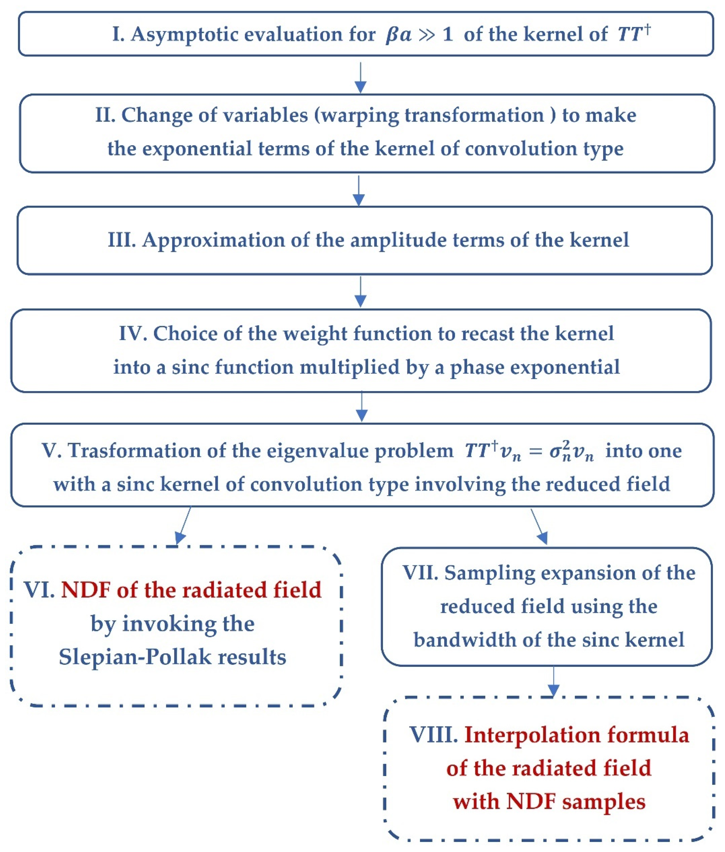
Figure 3.
Diagram in degrees of the function in terms of .
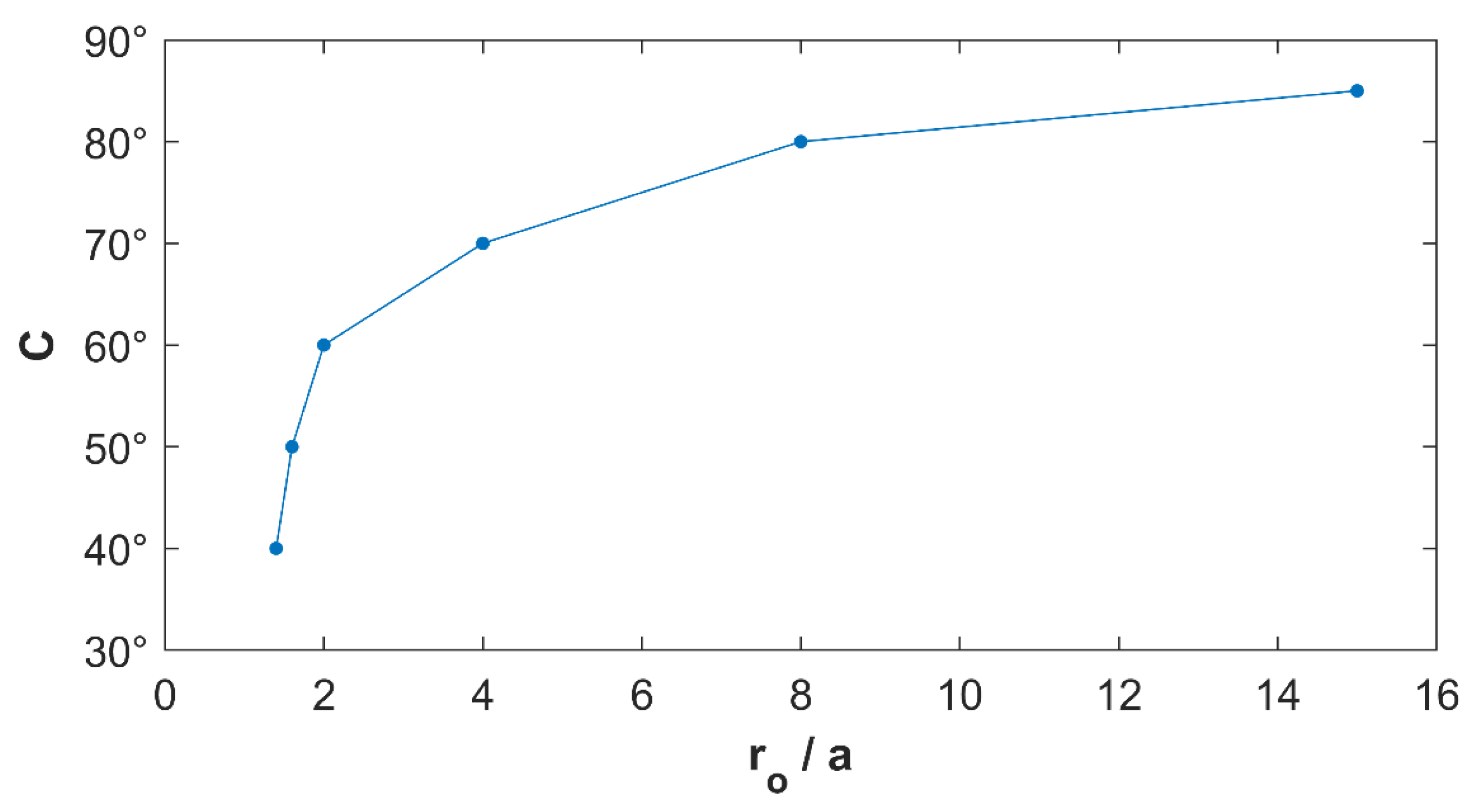
Figure 4.
Comparison between the singular values of the radiation operator and those obtained by introducing the weighted adjoint. The diagram refers to the configuration .
Figure 4.
Comparison between the singular values of the radiation operator and those obtained by introducing the weighted adjoint. The diagram refers to the configuration .
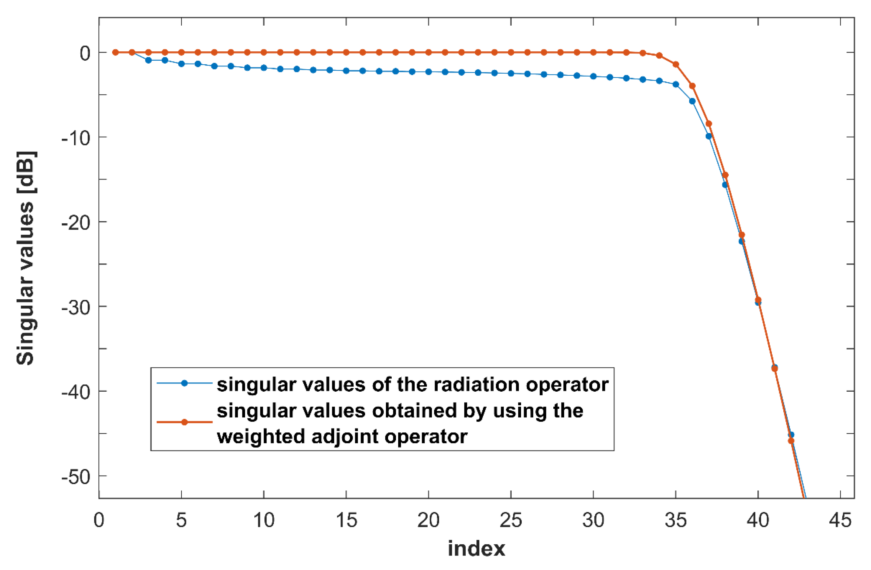
Figure 5.
Optimal position of the far-field samples in the variable . The diagram refers to the configuration .
Figure 5.
Optimal position of the far-field samples in the variable . The diagram refers to the configuration .
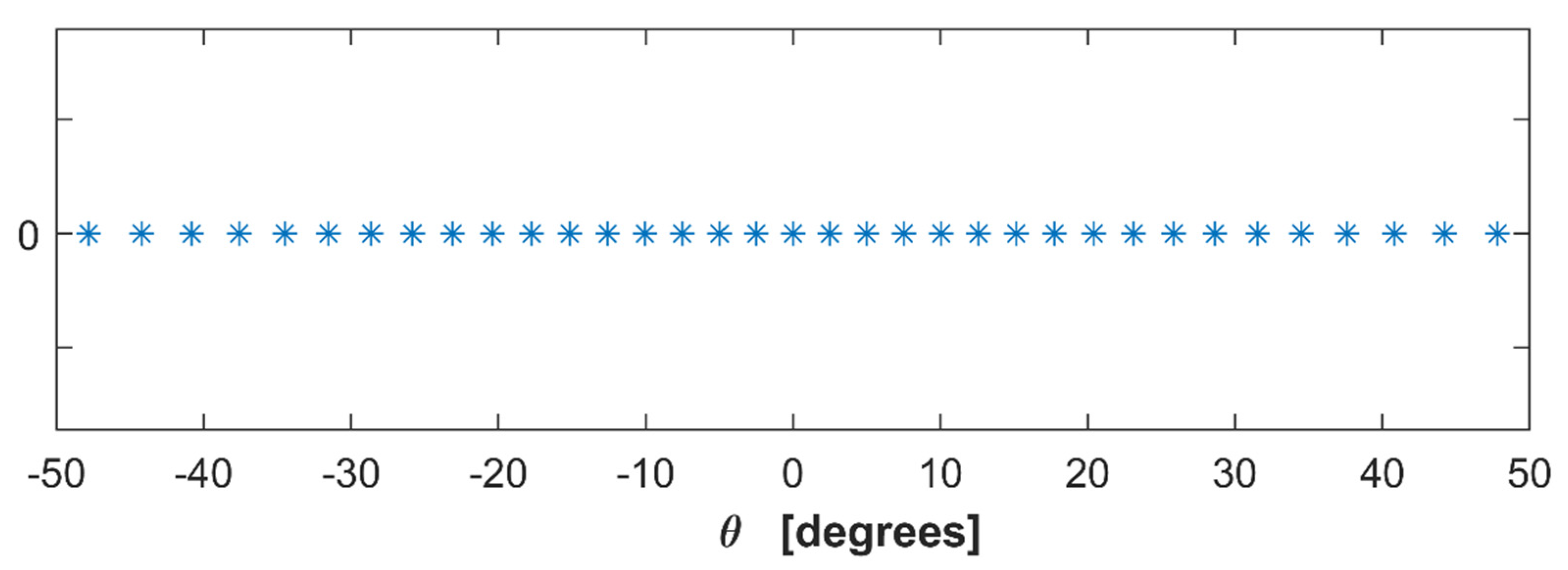
Figure 6.
Comparison between the far field computed by the radiation model in (2) and the far field returned by the interpolation Formula (32). The diagram refers to the configuration .
Figure 6.
Comparison between the far field computed by the radiation model in (2) and the far field returned by the interpolation Formula (32). The diagram refers to the configuration .

Figure 7.
Comparison between the exact far-field, the far-field obtained by the interpolation of uniform samples and the far field obtained by the interpolation of uniform samples. The diagram refers to the configuration .
Figure 7.
Comparison between the exact far-field, the far-field obtained by the interpolation of uniform samples and the far field obtained by the interpolation of uniform samples. The diagram refers to the configuration .

Figure 8.
Comparison between the singular values of the radiation operator and those obtained by introducing the weighted adjoint. The diagrams refer to the configuration , .
Figure 8.
Comparison between the singular values of the radiation operator and those obtained by introducing the weighted adjoint. The diagrams refer to the configuration , .
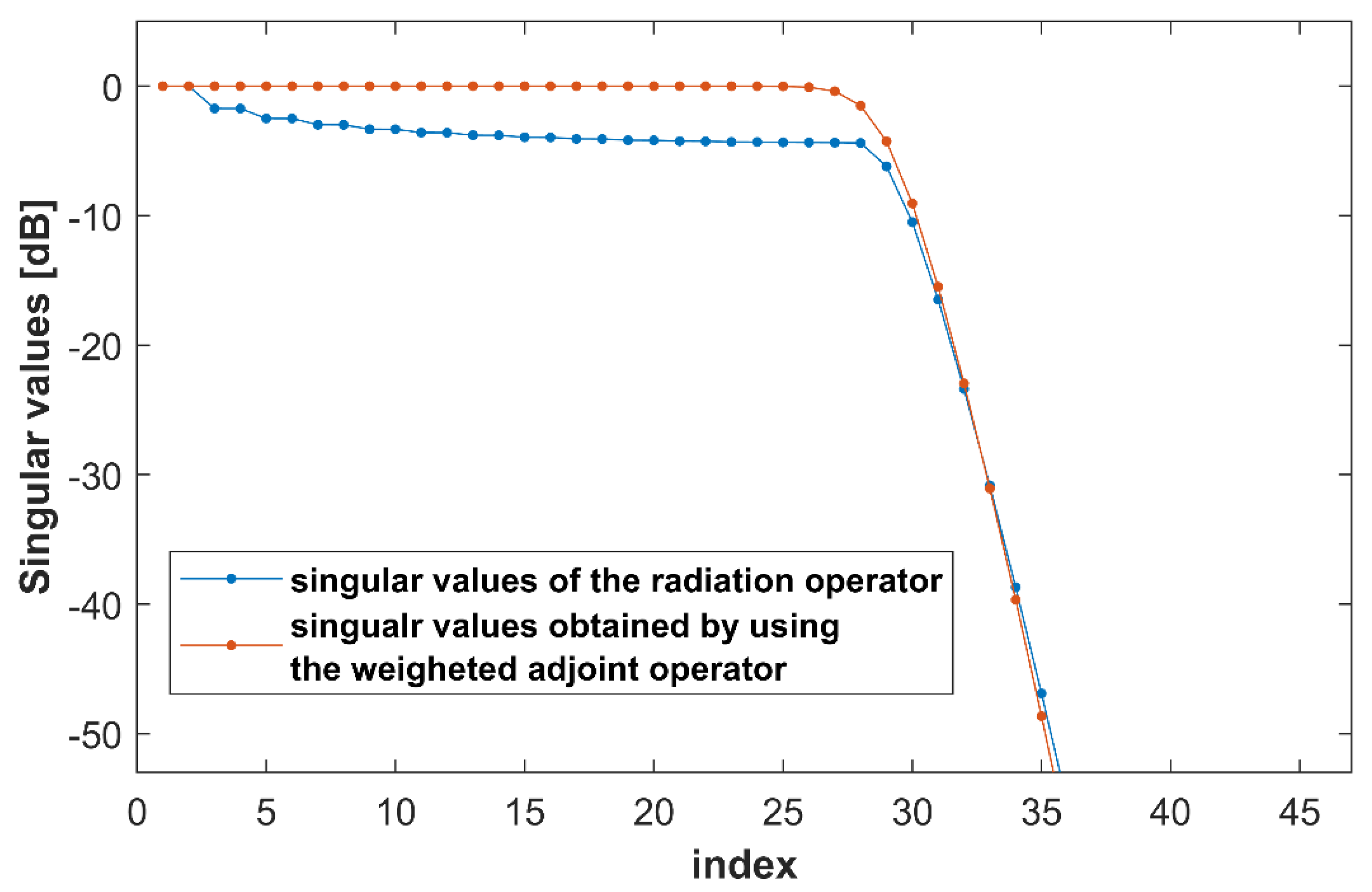
Figure 9.
Optimal position of the far-field samples in the variable . The diagram refers to the configuration .
Figure 9.
Optimal position of the far-field samples in the variable . The diagram refers to the configuration .

Figure 10.
Comparison between the far-field computed by the radiation model in (3) and the far-field returned by the interpolation Formula (57). The diagram refers to the configuration , .
Figure 10.
Comparison between the far-field computed by the radiation model in (3) and the far-field returned by the interpolation Formula (57). The diagram refers to the configuration , .

Figure 11.
Comparison between the exact near field, the near field obtained by the interpolation of uniform samples and the near field obtained by the interpolation of uniform samples. The diagram refers to the configuration .
Figure 11.
Comparison between the exact near field, the near field obtained by the interpolation of uniform samples and the near field obtained by the interpolation of uniform samples. The diagram refers to the configuration .

Table 1.
Values of C in terms of .
| 1.05 | |
| 1.22 | |
| 1.40 | |
| 1.48 |
Publisher’s Note: MDPI stays neutral with regard to jurisdictional claims in published maps and institutional affiliations. |
© 2022 by the authors. Licensee MDPI, Basel, Switzerland. This article is an open access article distributed under the terms and conditions of the Creative Commons Attribution (CC BY) license (https://creativecommons.org/licenses/by/4.0/).
Share and Cite
MDPI and ACS Style
Moretta, R.; Leone, G.; Munno, F.; Pierri, R. Optimal Field Sampling of Arc Sources via Asymptotic Study of the Radiation Operator. Electronics 2022, 11, 270. https://doi.org/10.3390/electronics11020270
AMA Style
Moretta R, Leone G, Munno F, Pierri R. Optimal Field Sampling of Arc Sources via Asymptotic Study of the Radiation Operator. Electronics. 2022; 11(2):270. https://doi.org/10.3390/electronics11020270
Chicago/Turabian StyleMoretta, Raffaele, Giovanni Leone, Fortuna Munno, and Rocco Pierri. 2022. "Optimal Field Sampling of Arc Sources via Asymptotic Study of the Radiation Operator" Electronics 11, no. 2: 270. https://doi.org/10.3390/electronics11020270
Note that from the first issue of 2016, this journal uses article numbers instead of page numbers. See further details here.