A Non-Local Tensor Completion Algorithm Based on Weighted Tensor Nuclear Norm

Abstract

In this paper, we proposed an image inpainting algorithm, including an interpolation step and a non-local tensor completion step based on a weighted tensor nuclear norm. Specifically, the proposed algorithm adopts the triangular based linear interpolation algorithm firstly to preform the observation image. Second, we extract the non-local similar patches in the image using the patch match algorithm and rearrange them to a similar tensor. Then, we use the tensor completion algorithm based on the weighted tensor nuclear norm to recover the similar tensors. Finally, we regroup all these recovered tensors to obtain the final recovered image. From the image inpainting experiments on color RGB images, we can see that the performance of the proposed algorithm on the peak signal-to-noise ratio (PSNR) and the relative standard error (RSE) are significantly better than other image inpainting methods.

1. Introduction

With the improvement of science and technology, more and more high-dimensional, data such as color images, videos and hyper-spectral images, are widely used. In practice, these high-dimensional data are usually stored as tensors [1]. For example, a color image can be represented as a third-order tensor, where the three dimensions are height, width and color channel. Unfortunately, it is unavoidable for images to be contaminated by noise during the process of storage and transmission. There are two main kinds of approaches to recover the incomplete image: the first kind is low-rank recovery, which mainly deals with small scratches or random missing pixels in incomplete images [2]; the second kind is based on deep learning, which is divided into convolutional neural network (CNNs)-based approaches and GAN-based approaches [3], where the goal is trying to use the known background of the image to fill in a big missing hole [4]. In this paper, we focus on the first kind of method that is recovering a degraded image with random missing pixels.

Recently, low-rank tensor recovery has been widely applied in image inpainting [2,5], background modeling [6], images and videos denoising [7,8], and other fields. Among the existing low-rank tensor recovery methods, tensor completion has been proposed to deal with the case of tensor data with missing entries. Tensor completion algorithm aims to recover a tensor from its incomplete or disturbed observations [2], formulated as follows.

$$arg\underset{\mathcal{X}}{min}\mathrm{rank}(\mathcal{X})s.t.{\mathrm{P}}_{\mathsf{\Omega }}\left(\mathcal{M}\right)={\mathrm{P}}_{\mathsf{\Omega }}\left(\mathcal{X}\right),$$

(1)

where $\mathcal{X}\in {\mathbb{R}}^{n_1\times n_2\times n_3}$, $\mathrm{rank}(·)$ denotes the tensor rank, and ${\mathrm{P}}_{\mathsf{\Omega }}\left(\mathcal{X}\right)$ denotes the projection of $\mathcal{X}$ on the observed set $\mathsf{\Omega }$.

Unlike the matrix rank, the definition of the tensor rank is still ambiguous and nonuniform. Depending on different tensor ranks, there are various tensor completion methods that can be derived. Traditionally, there are three types definitions of tensor rank, including the CP (CANDECOMP/PARAFAC) rank [9,10] based on the CP decomposition, the Tucker rank [10,11] based on Tucker decomposition, and the tensor tubal rank [12] based on tensor products. The CP rank is defined as the smallest number of the rank-one decomposition of the given tensor. Unfortunately, the minimization problem is NP-hard, which restricts the application of the CP rank [13]. The Tucker rank is a multi-linear rank formed by matrix rank, which is defined as a vector whose ith element equals the rank of the tensor’s mode-i unfolding matrix [14]. Since nuclear norm minimization is the most popular method for low-rank matrix completion. There are several notions of the tensor nuclear norm proposed. Liu et al. [15] proposed the sum of the unclear norm (SNN) as the convex surrogate of the Tucker rank. The proposal of SNN significantly improves the development of tensor recovery problems. Based on SNN, Zhang et al. [16,17] proposed a general framework merging the features of rectification and alignment for robust tensor recovery. Unfortunately, SNN is not a tight convex relaxation of the Tucker rank, and the balanced matricization strategy fails to exploit the structure information completely [18]. In recent years, Kilmer et al. [12] proposed the tensor tubal rank based on the tensor product, which is defined as the number of non-zero tensor singular tubes of the singular value tensor. As tensor tubal rank is discrete, Zhang et al. [2] proposed the tensor nuclear norm (TNN) as a convex relaxation of the tensor tube rank and applied it to the tensor completion algorithm.

However, since the singular values of natural images present a heavy-tailed distribution [19] in most cases, the tensor completion algorithm based on TNN minimization usually results in the over-penalty problem [20]. This problem will affect the effect of image recovery. To balance the effectiveness and solubility resulting from the algorithm based on TNN, Wang et al. [21] proposed a generalized non-convex approach for low-rank tensor recovery. This approach contains many non-convex relaxation strategies (such as $L_p$ norm [22], ETP [23], Geman [24], etc.) and converts the non-convex tubal rank minimization into the weighted tensor nuclear norm minimization. This method solved the over-penalty problem caused by the tensor nuclear norm, and achieved a stronger recovery capacity in recovery than TNN.

Unfortunately, the natural images usually do not satisfy the low-rank property. Since natural images have a high self-similarity property [25], the non-local means (NLM) algorithm [26] was proposed for solving the problem of natural image recovery. The NLM exploits the self-similarity inherent in images to estimate the pixels by weighted averaging all similar pixels, which can effectively improve the effect of the tensor completion algorithm. The self-similar property of the images has been widely used in the field of color images processing [27,28,29]. In addition, for medical images, such as MRI, the self-similarity also exists in each slices, and several studies [30] have utilized NLM to improve the effect of the medical image recovery. The recovered images or videos can be used in object detection [31] and object tracking [32].

Based on the above discussion, this paper proposed a non-local tensor completion algorithm based on weighted tensor nuclear norm (WNTC). Firstly, the WNTC algorithm pre-processes the images by interpolation to obtain better similar patches from a tensor and then stores these similar patches as tensors, called similar tensors. Then, we adopt the tensor completion algorithm based on the weighted tensor nuclear norm to recover all the similar tensors. Finally, regroup all completed tensors to obtain the image recovery result. Compared with other algorithms such as TNN [33], HaLRTC [15], FBCP [34] and Song [25], the proposed algorithm achieves better PSNR and RSE results and has better visual effects.

2. Notations and Preliminaries

2.1. Notations

In this paper, the fields of real numbers and complex numbers are denoted as $\mathbb{R}$ and $\mathbb{C}$, respectively, and we denote tensors by Euler script letters, e.g., $\mathcal{A}$; matrices are denoted by capital letters, e.g., A; sets are denoted by boldface capital letters, e.g., $\mathbf{A}$; vectors are denoted by boldface lowercase letters, e.g., $\mathbf{a}$, and scalars are denoted by lowercase letters e.g., a.

More definitions and symbols are given as follows: We denote a 3-order tensor as $\mathcal{A}\in {\mathbb{C}}^{n_1\times n_2\times n_3}$, where $n_k$$(k=1,2,3)$ is a positive integer. We denote Frobenius norm, $l_1$ norm, infinity norm and $l_0$ norm as ${\parallel \mathcal{A}\parallel }_F=\sqrt{{\sum }_{i_1,i_2,i_3}{\mathcal{A}}_{i_1{i}_2{i}_3}^2}$, ${\parallel \mathcal{A}\parallel }_1={\sum }_{i_1,i_2,i_3}\left|{\mathcal{A}}_{i_1{i}_2{i}_3}\right|$, ${\parallel \mathcal{A}\parallel }_{\infty }={max}_{i_1,i_2,i_3}\left|{\mathcal{A}}_{i_1{i}_2{i}_3}\right|$ and the number of nonzero entries of $\mathcal{A}$, respectively. For $\mathcal{A}$, $\mathcal{B}\in {\mathbb{C}}^{n_1\times n_2\times n_3}$, the inner product of $\mathcal{A}$ and $\mathcal{B}$ is denoted as $⟨\mathcal{A},\mathcal{B}⟩={\sum }_{i_1=1}^{n_1}{\sum }_{i_2=1}^{n_2}{\sum }_{i_3=1}^{n_3}$${\mathcal{A}}_{i_1{i}_2{i}_3}\mathrm{Conj}\left({\mathcal{B}}_{i_1{i}_2{i}_3}\right)$.

In addition, we follow the definitions in [35]: Use the Matlab notation $\mathcal{A}(i,:,:)$, $\mathcal{A}(:,i,:)$ and $\mathcal{A}(:,:,i)$ to denote, respectively, the i-th horizontal, lateral and frontal slice, and the frontal slice $\mathcal{A}(:,:,i)$ is denoted compactly as $A^{\left(i\right)}$. In addition, $\mathrm{bcirc}(·)$ and $\mathrm{bdiag}(·)$ are defined as

$\mathrm{bcirc}\left(\mathcal{A}\right)=\left(\begin{array}{cccc}{A}^{\left(1\right)}& A^{\left(n_3\right)}& \cdots & A^{\left(2\right)}\\ A^{\left(2\right)}& A^{\left(1\right)}& \cdots & A^{\left(3\right)}\\ ⋮& ⋮& \ddots & ⋮\\ A^{\left(n_3\right)}& A^{(n_3-1)}& \cdots & A^{\left(1\right)}\end{array}\right),$

$\mathrm{bdiag}\left(\mathcal{A}\right)=\left(\begin{array}{cccc}{A}^{\left(1\right)}& \mathbf{0}& \cdots & \mathbf{0}\\ \mathbf{0}& A^{\left(2\right)}& \cdots & \mathbf{0}\\ ⋮& ⋮& \ddots & ⋮\\ \mathbf{0}& \mathbf{0}& \cdots & A^{\left(n_3\right)}\end{array}\right).$

2.2. Preliminary Definitions and Results

Definition 1. 

(T-product) [36] Let $\mathcal{A}\in {\mathbb{R}}^{n_1\times n_2\times n_3}$ and $\mathcal{B}\in {\mathbb{R}}^{n_2\times l\times n_3}$. Then the $\mathrm{t}$-product $\mathcal{A}{\ast }_{\mathrm{t}}\mathcal{B}$ is defined to be a tensor of size $n_1\times l\times n_3$,

$$\mathcal{A}{\ast }_{\mathrm{t}}\mathcal{B}=\mathrm{fold}(\mathrm{bcirc}\left(\mathcal{A}\right)·\mathrm{unfold}\left(\mathcal{B}\right)).$$

(2)

Definition 2. 

(F-diagonal tensor) [36] Tensor $\mathcal{A}$ is called f-diagonal if each of its frontal slices is a diagonal matrix.

Definition 3. 

(Identity tensor) [36] The tensor $\mathcal{I}\in {\mathbb{R}}^{n\times n\times n_3}$ is the tensor with the first frontal slice being the identity matrix, and other frontal slices being all zeros.

Definition 4. 

(Conjugate transpose) [35] The conjugate transpose of a tensor $\mathcal{A}\in {\mathbb{C}}^{n_1\times n_2\times n_3}$ was the tensor ${\mathcal{A}}^{*}\in {\mathbb{C}}^{n_2\times n_1\times n_3}$ obtained by conjugate transposing each of the frontal slice and then reversing the order of transposed frontal slice from positions 2 through to $n_3$.

Definition 5. 

(Orthogonal tensor) [36] A tensor $\mathcal{Q}\in {\mathbb{C}}^{n\times n\times n_3}$ is orthogonal if it satisfies ${\mathcal{Q}}^{*}{\ast }_{\mathrm{t}}\mathcal{Q}=\mathcal{Q}{\ast }_{\mathrm{t}}{\mathcal{Q}}^{*}=\mathcal{I}$.

Theorem 1. 

(t-SVD) [35] Let $\mathcal{A}\in {\mathbb{R}}^{n_1\times n_2\times n_3}$. Then it can be factorized as $\mathcal{A}=\mathcal{U}{\ast }_{\mathrm{t}}\mathcal{S}{\ast }_{\mathrm{t}}{\mathcal{V}}^{*}$, where $\mathcal{U}\in {\mathbb{R}}^{n_1\times n_1\times n_3}$, $\mathcal{V}\in {\mathbb{R}}^{n_2\times n_2\times n_3}$ are orthogonal, and $\mathcal{S}\in {\mathbb{R}}^{n_1\times n_2\times n_3}$ is an f-diagonal tensor, see Algorithm 1 for details.

Definition 6. 

(Tensor tubal rank) [35] For $\mathcal{A}\in {\mathbb{R}}^{n_1\times n_2\times n_3}$, the tensor tubal rank, denoted by ${\mathrm{rank}}_{\mathrm{t}}\left(\mathcal{A}\right)$, is defined as the number of non-zero singular tubes of $\mathcal{S}$, where $\mathcal{S}$ is from the t-SVD of $\mathcal{A}=\mathcal{U}{\ast }_{\mathrm{t}}\mathcal{S}{\ast }_{\mathrm{t}}{\mathcal{V}}^{*}$. We can write ${\mathrm{rank}}_{\mathrm{t}}\left(\mathcal{A}\right)=\#\{i,\mathcal{S}(i,i,:)\ne \mathit{0}\}=\#\{i,\mathcal{S}(i,i,1)\ne 0\}$. Denote $\sigma \left(\mathcal{S}\right)={(\mathcal{S}(1,1,1),\mathcal{S}(2,2,1),...,\mathcal{S}(r,r,1))}^T$, in which $r={\mathrm{rank}}_t\left(\mathcal{A}\right)$.

Definition 7. 

(Tensor nuclear norm) [35] Let $\mathcal{A}=\mathcal{U}{\ast }_{\mathrm{t}}\mathcal{S}{\ast }_{\mathrm{t}}{\mathcal{V}}^{*}$ be the t-SVD of $\mathcal{A}\in {\mathbb{R}}^{n_1\times n_2\times n_3}$. Tensor nuclear norm of the tensor tubal rank, is defined as ${\parallel \mathcal{A}\parallel }_{*}=⟨\mathcal{S},\mathcal{I}⟩={\sum }_{i=1}^r\mathcal{S}(i,i,1)$, where $r={\mathrm{rank}}_t\left(\mathcal{A}\right)$.

Algorithm 1: t-SVD [35]

Input: $\mathcal{Y}\in {\mathbb{R}}^{n_1\times n_2\times n_3}$, $\lambda >0$. Output: $\mathcal{U}$, $\mathcal{S}$ and $\mathcal{V}$.  1. Compute $\overline{\mathcal{Y}}=\mathrm{fft}(\mathcal{Y},\left[\right],3)$.  2. Compute each frontal slice of $\overline{\mathcal{U}}$, $\overline{\mathcal{S}}$ and $\overline{\mathcal{V}}$ from $\overline{\mathcal{Y}}$ by    for $i=1,...,\lfloor \frac{n_3+1}{2}\rfloor$ do       $[{\overline{U}}^{\left(i\right)},{\overline{S}}^{\left(i\right)},{\overline{V}}^{\left(i\right)}]=\mathrm{SVD}\left({\overline{Y}}^{\left(i\right)}\right)$;    end for    for $i=\lfloor \frac{n_3+1}{2}\rfloor +1,\cdots ,n_3$ do       ${\overline{U}}^{\left(i\right)}=Conj\left({\overline{U}}^{(n_3-i+2)}\right)$;       ${\overline{S}}^{\left(i\right)}={\overline{S}}^{(n_3-i+2)}$;       ${\overline{V}}^{\left(i\right)}=Conj\left({\overline{V}}^{(n_3-i+2)}\right)$;    end for  3. $\mathcal{U}=\mathrm{ifft}(\overline{U},\left[\right],3)$, $\mathcal{S}=\mathrm{ifft}(\overline{S},\left[\right],3)$ and $\mathcal{V}=\mathrm{ifft}(\overline{V},\left[\right],3)$.

Tensor Completion Based on Weighted Tensor Nuclear Norm

To ensure the effectiveness of the tensor completion algorithm in image recovery, this paper uses the weighted tensor nuclear norm to approximate the tensor tubal rank, which is defined as:

Definition 8 

([21]). (Weighted tensor nuclear norm) For $\mathcal{X}\in {\mathbb{R}}^{n_1\times n_2\times n_3}$, its weighted tensor nuclear norm is defined as the weighted sum of all singular values of all frontal slices in the Fourier domain, that is ${∥\mathcal{X}∥}_{\mathbf{W},\ast }:=\frac{1}{n_3}{\displaystyle \sum _{i=1}^m}{\displaystyle \sum _{j=1}^{n_3}}{\omega }_{ij}{\sigma }_{ij},$ where the $m=min(n_1,n_2)$, the $\mathbf{W}=({\omega }_{ij}{)}_{m\times n_3}$ is a weighted matrix that denotes the weight of each singular values of the tensor, ${\sigma }_{ij}$ denotes the singular value of the tensor, ${\omega }_{ij}\in \partial \psi \left({\sigma }_{ij}\left(\mathcal{T}\right)\right)$ where the $\psi (·)$ is a non-convex surrogate function.

Using the weighted tensor nuclear norm denotes the tensor rank of $\mathcal{X}$ in Equation (1). Then the tensor completion model is written as:

$$arg\underset{\mathcal{X}}{min}{∥\mathcal{X}∥}_{\mathbf{W},\ast }s.t.{\mathrm{P}}_{\mathsf{\Omega }}\left(\mathcal{M}\right)={\mathrm{P}}_{\mathsf{\Omega }}\left(\mathcal{X}\right).$$

(3)

We call Equation (3) the weighted tensor nuclear norm-based tensor completion model, which is usually solved by the alternating direction method of multipliers (ADMM) [37]. To facilitate solving the model, we first rewrite Equation (3) into the following form:

$$arg\underset{\mathcal{X}}{min}{∥\mathcal{X}∥}_{\mathbf{W},\ast }+{\mathbf{1}}_{{\mathrm{P}}_{\mathsf{\Omega }}\left(\mathcal{X}\right)={\mathrm{P}}_{\mathsf{\Omega }}\left(\mathcal{M}\right)}\left(\mathcal{Z}\right)s.t.\mathcal{X}=\mathcal{Z},$$

(4)

where ${\mathbf{1}}_{{\mathrm{P}}_{\mathsf{\Omega }}\left(\mathcal{X}\right)={\mathrm{P}}_{\mathsf{\Omega }}\left(\mathcal{M}\right)}\left(\mathcal{Z}\right)$ denotes the indicator function (if the subscript condition of the $\mathbf{1}$ is satisfied, the indicator function denotes 0, and if it is non satisfied, it denotes 1). Based on Equation (4), an augmented Lagrangian function can be derived:

$$\begin{array}{c}{L}_{\rho }(\mathcal{X},\mathcal{Z},\mathcal{Q})={\left|\right|\mathcal{X}\left|\right|}_{\mathbf{W},\ast }+{\mathbf{1}}_{{\mathrm{P}}_{\mathsf{\Omega }}\left(\mathcal{X}\right)={\mathrm{P}}_{\mathsf{\Omega }}\left(\mathcal{M}\right)}\left(\mathcal{Z}\right)+\hfill \\ ⟨\mathcal{Q},\mathcal{X}-\mathcal{Z}⟩+\frac{1}{\rho }{\left|\right|\mathcal{X}-\mathcal{Z}+\mathcal{Q}\left|\right|}_F^2,\hfill \end{array}$$

(5)

where the $\rho$ is a parameter that controls the convergence, $\mathcal{Q}$ is the Lagrangian multiplier, and $⟨·,·⟩$ denotes the inner product. Equation (5) can be updated iteratively by the following steps. Step 1 Update ${\mathcal{X}}^{k+1}$ by

$$\begin{array}{c}{\mathcal{X}}^{k+1}=arg\underset{\mathcal{X}}{min}{∥\mathcal{X}∥}_{\mathbf{W},\ast }+⟨{\mathcal{Q}}^k,\mathcal{X}-{\mathcal{Z}}^k⟩+\frac{1}{{\rho }^k}{∥\mathcal{X}-{\mathcal{Z}}^k∥}_F^2\hfill \\ =arg\underset{\mathcal{X}}{min}{\rho }^k{\left|\right|\mathcal{X}\left|\right|}_{\mathbf{W},\ast }+\left|\right|\mathcal{X}-{\mathcal{Z}}^k+\frac{{\rho }^k}{2}{\mathcal{Q}}^k{\left|\right|}_F^2.\hfill \end{array}$$

(6)

The Equation (6) is calculated by the weighted tensor singular value threshold algorithm: ${\mathcal{X}}^{k+1}={\mathcal{D}}_{\mathbf{W},\tau }({\mathcal{Z}}^k-\frac{{\rho }^k}{2}{\mathcal{Q}}^k)$, where ${\mathcal{D}}_{\mathbf{W},\tau }(·)$ is the weighted tensor singular value shrinking operator.

Step 2 Update ${\mathcal{Z}}^{k+1}$ by

$${\mathcal{Z}}^{k+1}=arg\underset{\mathcal{Z}}{min}\left|\right|{\mathcal{X}}^{k+1}-(\mathcal{Z}+\frac{{\rho }^k}{2}{\mathcal{Q}}^k){\left|\right|}_F^2+{\mathbf{1}}_{{\mathrm{P}}_{\mathsf{\Omega }}\left(\mathcal{X}\right)={\mathrm{P}}_{\mathsf{\Omega }}\left(\mathcal{M}\right)}\left(\mathcal{Z}\right).$$

(7)

Calculate the above Equation (7) by the least squares projection with a constraint term.

Step 3 Update Lagrangian multiplier tensor ${\mathcal{Q}}^{k+1}$ by

$${\mathcal{Q}}^{k+1}={\mathcal{Q}}^k+{\rho }^k({\mathcal{X}}^{k+1}-{\mathcal{Z}}^{k+1})$$

(8)

Step 4 Update the weight matrix ${\mathbf{W}}^{k+1}$ by

$${\mathbf{W}}^{k+1}={({\omega }_{ij}^{k+1}\in \partial \psi \left({\sigma }_{ij}\left({\mathcal{X}}^{(k+1)}\right)\right))}_{m\times n_3}$$

(9)

where the k denotes the number of iterations. The overall algorithm is summarized in Algorithm 2.

Algorithm 2: Tensor completion based on weighted tensor nuclear norm

Input: Lagrangian multiplier tensor ${\mathcal{Q}}^0$, non-convex surrogate function $\psi (·)$. Initialize:${\mathcal{X}}^0=0$, ${\mathcal{Z}}^0=0$, ${\rho }^0=1E^{-4}$, $\epsilon =1E^{-5}$, $\mu =1.2$, $\tau >0$, maxIter = 200.       Output: The image ${\mathcal{X}}^{*}$ after completion. for$k=1:$ maxIter do    Update ${\mathcal{X}}^{k+1}$ by Equation (6);    Update ${\mathcal{Z}}^{k+1}$ by Equation (7);    Update Lagrangian multiplier ${\mathcal{Q}}^{k+1}$ by Equation (8);    Compute ${\rho }^{k+1}=\mu {\rho }^k$;    Update weight matrix ${\mathbf{W}}^{k+1}$ by Equation (9);    if ${∥{\mathcal{X}}^{k+1}-{\mathcal{X}}^k∥}_{\infty }\le \epsilon$ do       break;    end if end for

3. Proposed Algorithm Scheme

In this section, based on the self-similarity property of natural images and the weighted tensor nuclear norm, we establish the WNTC algorithm. This algorithm makes full use of the low-rank property of the similar tensor in the image and can obtain better image restoration results.

3.1. Image Pre-Processing

The result of the patch match algorithm will be affected by the missing elements of the observed image. Thus, the missing elements also lead to poor image recovery results. In this paper, we first pre-process [25] the observed image by channel, as shown in Figure 1. Denote the t-th channel in the observed tensor $\mathcal{X}\in {\mathbb{R}}^{n_1\times n_2\times n_3}$ as ${\mathbf{A}}_t^{n_1\times n_2}$, the set of observed elements position is denoted as $\mathsf{\Omega }$, and the set of unobserved elements position as $\overline{\mathsf{\Omega }}$. We use a triangular-based linear interpolation algorithm [38] to interpolate the missing positions in ${\mathbf{A}}_t$. Specifically, we know the coordinates of the three vertices $P^1,P^2,P^3$ of one triangle. There must exist u and v such that we can calculate the color at any point P inside the triangle. In our method, we extract three vertices from $\mathsf{\Omega }$ denoted as $P^1,P^2,P^3$. First compute $u,v$ by $\left\{\begin{array}{c}{P}_x=P_x^1+u{P}_x^2+v{P}_x^3\hfill \\ P_y=P_y^1+u{P}_y^2+v{P}_y^3\hfill \end{array}\right.$ where $P_x,P_y$ are coordinates of the point P. Then the color of P is determined by $P=P^1+u{P}^2+v{P}^3.$ Calculate the color of each point inside the $\overline{\mathsf{\Omega }}$ and replace the color in the missing position. We denote the image after interpolation as $\widehat{{\mathbf{A}}_t}$. Figure 1c is the result obtained after pre-processing.

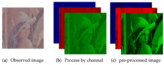
Figure 1. Pre-process observed image by channel.

3.2. Patch Match Algorithm

After the pre-processing, we apply the patch match algorithm to extract similar tensors from the $\widehat{\mathrm{A}}$. The main steps of the patch match algorithm are as follows. (1) For each point $P_i\in \overline{\mathsf{\Omega }}$, denote the ${\mathbf{M}}_{P_i}$ as the patch at the point $P_i$. If $P_i$ is so close to the edge of $\widehat{\mathrm{A}}$ that it can not obtain the $n\times n$ patch, then just use the patch near the edge. For example, if ${\left(P_i\right)}_x<n$, $n<{\left(P_i\right)}_y<n_2-n$, then use the patch centered at $(n,{\left(P_i\right)}_y)$. (2) Then traverse in a $N\times N$ search window with a step size of s pixel, and extract all candidate patches from the search window. (3) Then we find a set of similar patches of ${\mathbf{M}}_{P_i}$ in $\widehat{\mathrm{A}}$ by Euclidean distance (i.e., $\left|\right|{\mathbf{M}}_{P_i}-{\mathbf{M}}_Q{\left|\right|}_F$ where ${\mathbf{M}}_Q$ is a candidate patch). (4) We select the $T-1$ most similar candidate patches. After the steps above, we obtain a set of patches from $\widehat{\mathrm{A}}$. Let ${\mathbf{M}}_{P_i}$ be the first matrix in the group and we rearrange the matrices to a tensor ${\mathcal{M}}_i$, where ${\mathcal{M}}_i(:,:,k)(k=1,\cdots ,T)$ is the kth patch in the group. We call the tensor ${\mathcal{M}}_i$ similar tensor. We denote the set of observed elements position in the extracted similar tensor as ${\mathsf{\Omega }}_i^{\prime }$. Figure 2 shows the process of the patch match algorithm.

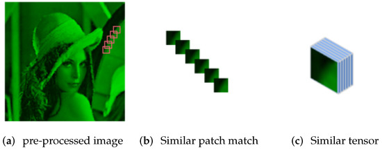
Figure 2. Process of patch matching.

3.3. Wntc Algorithm

For each ${\mathcal{M}}_i$, we recover it through the tensor completion algorithm based on the weighted tensor nuclear norm. The Equation (3) can be written as follows.

$${\widehat{\mathcal{X}}}_i=arg\underset{\mathcal{X}}{min}{∥\mathcal{X}∥}_{\mathbf{W},\ast }s.t.{\mathrm{P}}_{{{\mathsf{\Omega }}^{\prime }}_i}\left(\mathcal{X}\right)={\mathrm{P}}_{{{\mathsf{\Omega }}^{\prime }}_i}\left({\mathcal{M}}_i\right),$$

(10)

The tensor $\widehat{{\mathcal{X}}_i}$ is obtained by solving Equation (10) through Algorithm 2.

By regrouping the recovered tensor ${\widehat{\mathcal{X}}}_i$, we obtain the image recovery result ${\mathcal{A}}^{*}$. See Algorithm 3 for details of the WNTC algorithm.

Algorithm 3: WNTC Algorithm

Input: Color image $\mathcal{A}\in {\mathbb{R}}^{n_1\times n_2\times n_3}$, the set of observed element positions $\mathsf{\Omega }$, n, N, number of similar patch T and step s. Output: The color image ${\mathcal{X}}^{*}$ after completion. for$t=1:n_3$do    ${\mathbf{A}}_t=\mathcal{A}(:,:,\mathrm{t})$;    Pre-process the ${\mathbf{A}}_{\mathbf{t}}$ by triangular-based linear interpolation to obtain ${\widehat{\mathbf{A}}}_t$;    for each point $P_i$ of $\overline{\mathsf{\Omega }}$ do       Extract similar tensor $\mathcal{M}{}_i\in {\mathbb{R}}^{n\times n\times T}$ by patch match algorithm;       Complete ${\mathcal{M}}_i$ by Algorithm 2 to obtain $\widehat{{\mathcal{X}}_i}$;    end for    Regroup the tensor $\widehat{{\mathcal{X}}_i}$ to obtain the recovered tensor ${\mathcal{A}}^{*}$; end for

Experiments

In this section, we apply the WNTC algorithm to image inpainting applications and compare it with other methods, including three traditional low-rank tensor completion models: TNN [33], HaLRTC [15], FBCP [34], and three non-local tensor completion models: NL-HaLRTC, NL-FBCP, and Song [25]. In this paper, all the simulations were conducted on a PC with an Intel Xeon E5-2630v4@2.2GHz CPU and 128 G memory.

3.4. Parameter Setting

In this experiment, we set the non-convex surrogate function $\psi (·)$ as $L_p$ norm, where the parameter p is set to 0.4. Experiments show that the similar patch size n and similar patch number T have a significant impact on the performance of the WNTC algorithm. If n is set too large, it will be difficult to match a similar patch. A too large T will cause the similar tensor to contain too much redundant information, thus affecting the effectiveness of image recovery. Combining the accuracy of the results and time consumption, we set the similar patch size as $n=20$ and the number of similar patches as $T=5$ in this experiment. The image recovery performances are evaluated by the PSNR and RSE. Assuming $\mathcal{T}\in {\mathbb{R}}^{n_1\times n_2\times n_3}$ is the original image, $\widehat{\mathcal{T}}$ is the recovered image. The PSNR is defined as: $\mathrm{PSNR}=10{log}_{10}\left(\frac{n_1{n}_2{n}_3{∥\mathcal{T}∥}_{\infty }^2}{{∥\widehat{\mathcal{T}}-\mathcal{T}∥}_F^2}\right),$ The definition of RSE is: $\mathrm{RSE}=\left|\right|\mathcal{T}-\widehat{\mathcal{T}}{\left|\right|}_{\mathrm{F}}/{\left|\right|\mathcal{T}\left|\right|}_{\mathrm{F}}.$ Larger values of PSNR and lower values of RSE indicate better image recovery performance.

3.5. Color Image Inpainting

In this experiment, under different sampling rates, the WNTC algorithm and the other six tensor completion methods are, respectively, applied to recover the eight standard color images with a size of $256\times 256\times 3$. The eight color images are shown in Figure 3. The experimental results over selected eight color images under different sampling rates are shown in Table 1 (bold font indicates the best result). From this table, we can find that the WNTC algorithm achieved the best RSE result under different sampling rates; compared to the three non-local based methods, NL-HaLRTC, NL-FBCP, and Song, the WNTC algorithm significantly achieves higher PSNR in most cases. In addition, the PSNR of the WNTC algorithm is at least 4 db higher compared to the three methods that do not use the non-local strategy (TNN, HaLRTC and FBCP).

Figure 3. Eight color RGB pictures.

Table 1. PSNR and RSE results of different image recovery algorithm.

Sampling Rate	Image	FBCP		HaLRTC		TNN		NL-FBCP		NL-HaLRTC		Song		WNTC
		RSE	PSNR	RSE	PSNR	RSE	PSNR	RSE	PSNR	RSE	PSNR	RSE	PSNR	RSE	PSNR
0.2	Lena	0.200	19.26	0.396	13.86	0.131	23.04	0.099	25.29	0.115	24.42	0.077	27.43	0.076	27.55
	A.ort	0.136	19.33	0.208	15.79	0.100	22.00	0.085	23.44	0.099	22.40	0.070	25.01	0.069	25.18
	B.oon	0.232	18.29	0.369	14.66	0.198	19.81	0.167	20.49	0.186	20.69	0.145	22.27	0.145	22.23
	B.ara	0.249	18.57	0.405	14.80	0.162	22.36	0.116	25.01	0.149	23.43	0.102	26.18	0.099	26.38
	House	0.163	20.17	0.327	14.53	0.101	24.42	0.071	27.31	0.101	24.68	0.066	28.03	0.061	28.61
	P.ers	0.271	16.84	0.510	12.13	0.197	19.79	0.109	24.58	0.132	23.39	0.088	26.41	0.086	26.62
	S.oat	0.229	17.92	0.468	12.38	0.174	20.40	0.153	21.45	0.159	21.46	0.120	23.41	0.118	23.50
	Woman	0.172	21.24	0.406	14.40	0.121	24.43	0.100	25.98	0.140	23.63	0.062	30.04	0.055	31.13
	avg	0.207	18.95	0.386	14.07	0.148	22.03	0.112	24.19	0.135	23.01	0.091	26.10	0.089	26.40
0.3	Lena	0.195	19.49	0.365	14.48	0.094	25.82	0.075	27.70	0.086	26.80	0.063	29.24	0.061	29.40
	A.ort	0.135	19.36	0.192	16.41	0.074	24.65	0.078	24.10	0.076	24.53	0.057	26.85	0.055	27.08
	B.oon	0.223	18.60	0.340	15.27	0.160	21.54	0.150	21.95	0.158	21.96	0.128	23.33	0.128	23.28
	B.ara	0.247	18.64	0.373	15.42	0.114	25.26	0.100	26.32	0.113	25.59	0.085	27.75	0.081	28.05
	House	0.156	20.55	0.303	15.14	0.071	27.39	0.053	29.77	0.073	27.39	0.052	30.02	0.047	30.87
	P.ers	0.282	16.52	0.467	12.73	0.135	22.84	0.084	26.75	0.100	25.57	0.071	28.25	0.069	28.49
	S.oat	0.221	18.22	0.431	12.99	0.132	22.66	0.119	23.47	0.128	23.14	0.098	25.13	0.097	25.19
	Woman	0.179	20.96	0.374	15.00	0.087	27.17	0.058	30.61	0.098	26.48	0.050	31.90	0.042	33.47
	avg	0.205	19.04	0.356	14.68	0.108	24.67	0.090	26.33	0.104	25.18	0.075	27.81	0.073	28.23

To further illustrate the superiority of the WNTC algorithm, we take the color image ’house’ as an example. In Figure 4, we illustrate the comparison curves of PSNR obtained by the WNTC algorithm and other methods at different sampling rates. We can see from this figure that the WNTC algorithm achieves the best PSNR at five sampling rates from $0.1$ to $0.5$. In addition, the recovery performance of the non-local based tensor completion algorithm improves significantly with the increase in the sampling rate.

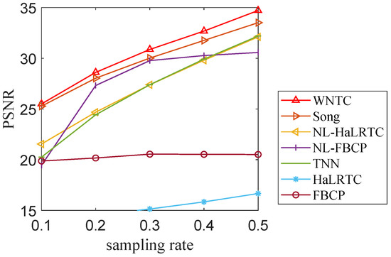
Figure 4. Curves of PSNR values of different algorithms.

In Figure 5, we present the visual results of image restoration for two images (Woman and House) with different algorithms at a sampling rate of 0.2. This figure shows that the WNTC algorithm can recover the edge and texture features of images well at a low sampling rate (e.g., the face of the person and the outline of the house). This is because the non-local similar tensor has better low-rank property, which makes the tensor completion algorithm more effective. Meanwhile, it is efficient to avoid the global distortion of an image by using the non-local strategy.

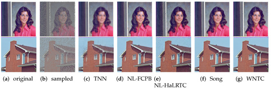
Figure 5. Recovery results of different algorithms on Woman and House images when sampling rate is 0.3.

4. Conclusions

This paper proposed a non-local tensor completion algorithm based on the weighted tensor nuclear norm and applied it to color image inpainting applications. This algorithm replaces the TNN with the weighted tensor nuclear norm to approximate the tensor tubal rank, which improves the efficiency of low-rank tensor recovery. Meanwhile, inspired by the non-local similarity of images, we have improved the patch match algorithm. Our WNTC algorithm pre-processes the observed image first in order to enhance the performance of the match. The experimental results show that our WNTC algorithm has good performance in color images inpainting at different sampling rates, with excellent PSNR and RSE results and good visual effects.

References

- Cichocki, A.; Mandic, D.; De Lathauwer, L.; Zhou, G.; Zhao, Q.; Caiafa, C.; Phan, H.A. Tensor decompositions for signal processing applications: From two-way to multiway component analysis. IEEE Signal Process. Mag. 2015, 32, 145–163. [Google Scholar] [CrossRef]
- Zhang, Z.; Ely, G.; Aeron, S.; Hao, N.; Kilmer, M. Novel methods for multilinear data completion and de-noising based on tensor-SVD. In Proceedings of the IEEE conference on Computer Vision and Pattern Recognition, Columbus, OH, USA, 23–28 June 2014; pp. 3842–3849. [Google Scholar]
- Elharrouss, O.; Almaadeed, N.; Al-Maadeed, S.; Akbari, Y. Image inpainting: A review. Neural Process. Lett. 2020, 51, 2007–2028. [Google Scholar] [CrossRef]
- Wang, Y.; Tao, X.; Qi, X.; Shen, X.; Jia, J. Image inpainting via generative multi-column convolutional neural networks. Adv. Neural Inf. Process. Syst. 2018, 31, 329–338. [Google Scholar]
- Heidel, G.; Schulz, V. A Riemannian trust-region method for low-rank tensor completion. Numer. Linear Algebra Appl. 2018, 25, e2175. [Google Scholar] [CrossRef]
- Zhang, X.; Zheng, J.; Zhao, L.; Zhou, Z.; Lin, Z. Tensor Recovery with Weighted Tensor Average Rank. IEEE Trans. Neural Netw. Learn. Syst. 2022, in press. [Google Scholar] [CrossRef] [PubMed]
- Zhang, X.; Zheng, J.; Wang, D.; Zhao, L. Exemplar-based denoising: A unified low-rank recovery framework. IEEE Trans. Circuits Syst. Video Technol. 2019, 30, 2538–2549. [Google Scholar] [CrossRef]
- Zheng, J.; Zhang, X.; Wang, W.; Jiang, X. Handling Slice Permutations Variability in Tensor Recovery. Proc. AAAI Conf. Artif. Intell. 2022, 36, 3499–3507. [Google Scholar] [CrossRef]
- Carroll, J.D.; Chang, J.J. Analysis of individual differences in multidimensional scaling via an N-way generalization of “Eckart-Young” decomposition. Psychometrika 1970, 35, 283–319. [Google Scholar] [CrossRef]
- Kolda, T.G.; Bader, B.W. Tensor decompositions and applications. SIAM Rev. 2009, 51, 455–500. [Google Scholar] [CrossRef]
- De Lathauwer, L.; De Moor, B.; Vandewalle, J. A multilinear singular value decomposition. SIAM J. Matrix Anal. Appl. 2000, 21, 1253–1278. [Google Scholar] [CrossRef]
- Kilmer, M.E.; Braman, K.; Hao, N.; Hoover, R.C. Third-order tensors as operators on matrices: A theoretical and computational framework with applications in imaging. SIAM J. Matrix Anal. Appl. 2013, 34, 148–172. [Google Scholar] [CrossRef]
- Hillar, C.J.; Lim, L.H. Most tensor problems are NP-hard. J. ACM (JACM) 2013, 60, 1–39. [Google Scholar] [CrossRef]
- Tucker, L.R. Some mathematical notes on three-mode factor analysis. Psychometrika 1966, 31, 279–311. [Google Scholar] [CrossRef]
- Liu, J.; Musialski, P.; Wonka, P.; Ye, J. Tensor completion for estimating missing values in visual data. IEEE Trans. Pattern Anal. Mach. Intell. 2012, 35, 208–220. [Google Scholar] [CrossRef] [PubMed]
- Zhang, X.; Wang, D.; Zhou, Z.; Ma, Y. Simultaneous rectification and alignment via robust recovery of low-rank tensors. Adv. Neural Inf. Process. Syst. 2013, 26, 1637–1645. [Google Scholar]
- Zhang, X.; Wang, D.; Zhou, Z.; Ma, Y. Robust low-rank tensor recovery with rectification and alignment. IEEE Trans. Pattern Anal. Mach. Intell. 2019, 43, 238–255. [Google Scholar] [CrossRef]
- Romera-Paredes, B.; Pontil, M. A new convex relaxation for tensor completion. Adv. Neural Inf. Process. Syst. 2013, 26, 2967–2975. [Google Scholar]
- Shang, F.; Cheng, J.; Liu, Y.; Luo, Z.Q.; Lin, Z. Bilinear factor matrix norm minimization for robust PCA: Algorithms and applications. IEEE Trans. Pattern Anal. Mach. Intell. 2017, 40, 2066–2080. [Google Scholar] [CrossRef]
- Sun, M.; Zhao, L.; Zheng, J.; Xu, J. A Nonlocal Denoising Framework Based on Tensor Robust Principal Component Analysis with lp norm. In Proceedings of the 2020 IEEE International Conference on Big Data (Big Data), Atlanta, GA, USA, 10–13 December 2020; pp. 3333–3340. [Google Scholar]
- Wang, H.; Zhang, F.; Wang, J.; Huang, T.; Huang, J.; Liu, X. Generalized nonconvex approach for low-tubal-rank tensor recovery. IEEE Trans. Neural Netw. Learn. Syst. 2021, 33, 3305–3319. [Google Scholar] [CrossRef]
- Frank, L.E.; Friedman, J.H. A statistical view of some chemometrics regression tools. Technometrics 1993, 35, 109–135. [Google Scholar] [CrossRef]
- Gao, C.; Wang, N.; Yu, Q.; Zhang, Z. A feasible nonconvex relaxation approach to feature selection. Proc. AAAI Conf. Artif. Intell. 2011, 25, 356–361. [Google Scholar] [CrossRef]
- Geman, D.; Reynolds, G. Constrained restoration and the recovery of discontinuities. IEEE Trans. Pattern Anal. Mach. Intell. 1992, 14, 367–383. [Google Scholar] [CrossRef]
- Song, L.; Du, B.; Zhang, L.; Zhang, L.; Wu, J.; Li, X. Nonlocal patch based t-svd for image inpainting: Algorithm and error analysis. Proc. AAAI Conf. Artif. Intell. 2018, 32, 2419–2426. [Google Scholar] [CrossRef]
- Buades, A.; Coll, B.; Morel, J.M. A review of image denoising algorithms, with a new one. Multiscale Model. Simul. 2005, 4, 490–530. [Google Scholar] [CrossRef]
- Xie, T.; Li, S.; Fang, L.; Liu, L. Tensor completion via nonlocal low-rank regularization. IEEE Trans. Cybern. 2018, 49, 2344–2354. [Google Scholar] [CrossRef]
- Zhao, X.L.; Yang, J.H.; Ma, T.H.; Jiang, T.X.; Ng, M.K.; Huang, T.Z. Tensor completion via complementary global, local, and nonlocal priors. IEEE Trans. Image Process. 2021, 31, 984–999. [Google Scholar] [CrossRef]
- Zhang, L.; Song, L.; Du, B.; Zhang, Y. Nonlocal low-rank tensor completion for visual data. IEEE Trans. Cybern. 2019, 51, 673–685. [Google Scholar] [CrossRef]
- Zhang, Y.; Wu, G.; Yap, P.T.; Feng, Q.; Lian, J.; Chen, W.; Shen, D. Hierarchical patch-based sparse representation—A new approach for resolution enhancement of 4D-CT lung data. IEEE Trans. Med. Imaging 2012, 31, 1993–2005. [Google Scholar] [CrossRef]
- Zhou, X.; Yang, C.; Yu, W. Moving Object Detection by Detecting Contiguous Outliers in the Low-Rank Representation. IEEE Trans. Pattern Anal. Mach. Intell. 2013, 35, 597–610. [Google Scholar] [CrossRef]
- Chan, S.; Jia, Y.; Zhou, X.; Bai, C.; Chen, S.; Zhang, X. Online Multiple Object Tracking Using Joint Detection and Embedding Network. Pattern Recognit. 2022, 130, 108793. [Google Scholar] [CrossRef]
- Lu, C.; Feng, J.; Lin, Z.; Yan, S. Exact low tubal rank tensor recovery from Gaussian measurements. arXiv 2018, arXiv:1806.02511. [Google Scholar]
- Zhao, Q.; Zhang, L.; Cichocki, A. Bayesian CP factorization of incomplete tensors with automatic rank determination. IEEE Trans. Pattern Anal. Mach. Intell. 2015, 37, 1751–1763. [Google Scholar] [CrossRef] [PubMed]
- Lu, C.; Feng, J.; Chen, Y.; Liu, W.; Lin, Z.; Yan, S. Tensor robust principal component analysis with a new tensor nuclear norm. IEEE Trans. Pattern Anal. Mach. Intell. 2019, 42, 925–938. [Google Scholar] [CrossRef] [PubMed]
- Kilmer, M.E.; Martin, C.D. Factorization strategies for third-order tensors. Linear Algebra Its Appl. 2011, 435, 641–658. [Google Scholar] [CrossRef]
- Zhang, Z.; Aeron, S. Exact tensor completion using t-SVD. IEEE Trans. Signal Process. 2016, 65, 1511–1526. [Google Scholar] [CrossRef]
- Watson, D.; Philip, G. Triangle based interpolation. J. Int. Assoc. Math. Geol. 1984, 16, 779–795. [Google Scholar] [CrossRef]
Publisher’s Note: MDPI stays neutral with regard to jurisdictional claims in published maps and institutional affiliations. |
© 2022 by the authors. Licensee MDPI, Basel, Switzerland. This article is an open access article distributed under the terms and conditions of the Creative Commons Attribution (CC BY) license (https://creativecommons.org/licenses/by/4.0/).