
Depth Image Denoising Algorithm Based on Fractional Calculus


1
School of Electronics and Information Engineering, Changchun University of Science and Technology, Changchun 130022, China
2
Xi’an Key Laboratory of Active Photoelectric Imaging Detection Technology, Xi’an Technological University, Xi’an 710021, China
*
Authors to whom correspondence should be addressed.
Electronics 2022, 11(12), 1910; https://doi.org/10.3390/electronics11121910
Submission received: 24 May 2022
/
Revised: 15 June 2022
/
Accepted: 16 June 2022
/
Published: 19 June 2022
(This article belongs to the Special Issue Edge Computing for Urban Internet of Things)
Abstract
:Depth images are often accompanied by unavoidable and unpredictable noise. Depth image denoising algorithms mainly attempt to fill hole data and optimise edges. In this paper, we study in detail the problem of effectively filtering the data of depth images under noise interference. The classical filtering algorithm tends to blur edge and texture information, whereas the fractional integral operator can retain more edge and texture information. In this paper, the Grünwald–Letnikov-type fractional integral denoising operator is introduced into the depth image denoising process, and the convolution template of this operator is studied and improved upon to build a fractional integral denoising model and algorithm for depth image denoising. Depth images from the Redwood dataset were used to add noise, and the mask constructed by the fractional integral denoising operator was used to denoise the images by convolution. The experimental results show that the fractional integration order with the best denoising effect was −0.4 ≤ ν ≤ −0.3 and that the peak signal-to-noise ratio was improved by +3 to +6 dB. Under the same environment, median filter denoising had −15 to −30 dB distortion. The filtered depth image was converted to a point cloud image, from which the denoising effect was subjectively evaluated. Overall, the results prove that the fractional integral denoising operator can effectively handle noise in depth images while preserving their edge and texture information and thus has an excellent denoising effect.
1. Introduction
The current, rapidly developing era of artificial intelligence, intelligent driving, and 3D reconstruction research is founded on the availability of high-precision, high-quality depth data. Depth data are represented in depth images, which are acquired through methods such as stereo matching, lidar, and depth camera-based imaging. Although depth cameras can acquire images in real time, most depth camera images are highly sensitive to environmental factors that introduce noise, producing images with low resolution and quality. Removing the noise in these images can greatly improve super-resolution reconstruction. Research has imitated the degradation process of Kinect to generate depth images for testing [1]. For prospective applications in depth image super-resolution reconstruction and 3D reconstruction [2,3], depth image noise processing forms a crucial pre-link [4,5,6,7,8,9,10,11] and has been the focus of research on effective depth image noise processing algorithms.
Currently, depth image denoising algorithms mainly have two modes: non-colour image auxiliary filtering and colour image auxiliary filtering. References [4,5,6,7] proposed the use of the ordinary image filter method to denoise depth images, an approach that repairs the depth map image but with the loss of much edge information. References [8,9,10,11,12] reported on a denoising method that uses the image median filter to filter the pixel values in the depth image and then superimposes the image enhancement. Reference [12] proposed depth image denoising by combining the colour image auxiliary guide filter to smooth the depth image; unfortunately, this restoration approach destroys part of the original depth values. Reference [13] proposed a denoising method that uses deep learning to improve the quality of depth images. However, in this approach, the denoising effect is evaluated solely visually, as the focus is on filling in holes in the depth image to improve target recognition and detection based on depth images. Detection and denoising algorithms can also blur the texture information of depth images. In summary, no optimal depth image processing method has yet been developed, as the numerous available methods are each lacking in some aspect(s). In particular, in the depth image filtering algorithms guided by achromatic images, the edge smoothing process destroys some valid and useful data. The algorithms can remove noise to varying degrees, but they often also remove information such as edge and texture details, which are critical components of depth images. The root cause of this problem is that the denoising operator constructed using the integer-order integral severely reduces the high-frequency information in the image, resulting in the loss of much of this critical information in the denoised image. The application of fractional calculus to image processing has been studied for several years [13,14,15,16,17]. For example, reference [18] successfully applied fractional calculus to the shadow detection of depth images, demonstrating how fractional calculus can be applied to depth images. Although the integer-order filtering algorithm has limitations, it can be optimised by introducing a fractional-order integral model, which is a significant development in the field of depth image denoising algorithms.
Based on the characteristics of fractional calculus, Section 2 deduces the fractional-order integral operator suitable for image processing and constructs a fractional-order integral denoising operator.
Section 3 compares the processing effects of the fractional integral filtering algorithm and median filtering. Simulations show that fractional integral filtering has a stronger noise filtering effect and that it retains more texture information than does median filtering. Comparisons of the proposed algorithm with the classical image denoising algorithms (median filtering and Gaussian filtering) show that the classical algorithms have a relatively high distortion degree. The algorithms are also compared with respect to the distortion of the original noise image, focusing on the distortion of the data point cloud image after Gaussian filtering; the results show that after Gaussian filtering, the degree of distortion is larger by approximately 15–30 dB. Therefore, only the median filter is used as a reference comparison.
2. Fractional Calculus Operator Denoising Theory and Method
Integer-order calculus can describe phenomena very well, whereas fractional-order calculus can observe the world from another perspective and obtain information that integer-order calculus cannot. Integer-order calculus has a clear physical meaning and geometric interpretation, whereas attributing clear physical and geometric meanings to fractional-order calculus has been difficult. Scientists have comprehensively examined this problem from different perspectives and have obtained a diverse set of results. Most of these results are from special cases of fractional calculus, which limits their wider applicability. Podlubny [19] first proposed a physical explanation of fractional calculus in 2001. In physics, personal time τ and cosmic time T are two distinct concepts. Universal time is uniform and equally spaced elapsed time (absolute time), whereas personal time is non-uniform time (relative time). Podlubny asserted that fractional differentiation corresponds to the physical phenomenon of τ observed from the perspective of T.
Fractional calculus is suitable for describing some physical phenomena that cannot be fully described by integer calculus. The description of fractional calculus covers a wide range of physical fields—for example, anomalous diffusion, random walks, viscoelastic dynamics, automatic control PID, signal processing, neural networks, chaotic systems, and image processing.
2.1. Effect of Fractional Integration on Signal and Model Construction
For the energy signal of any square area, the Fourier transform is derived from the basic theory of signal processing as
Assuming the fractional ν-th order derivative of the signal , according to the Fourier transform, we get
In
In Figure 1, the fractional differential operator is an amplitude–frequency curve in the range of [−2, 2]. Order v = 0 means that the signal does not change. When the order is less than zero (−2 < v < 0), the signal represents an integral operation. The figure shows that the signal can be nonlinearly attenuated, and the amplitude of this attenuation is related to the differential order. When the order is greater than zero (0 < v < 2), the signal represents a differential operation with enhanced nonlinearity: the greater the differential order, the greater the enhancement amplitude. This feature of fractional-order calculus is applied in the image field. To achieve more prominent image edges and retain the texture information of the smooth area of the image, the fractional derivative can be used to improve the high-frequency components while also nonlinearly retaining the special characteristics of the low-frequency components of the signal. When it is instead necessary to denoise the image while retaining much of the edge and texture information, the opposing characteristics of fractional integration and differentiation can be used to nonlinearly retain the highest frequency components while attenuating the low-frequency component of the signal. Integral image denoising can thus achieve image denoising while preserving as much image edge and texture information as possible, as shown in Figure 1.
2.2. Construction Based on Fractional Integral Operator
The Grünwald–Letnikov (G-L) definition of fractional calculus is
where is the fractional order, h is the calculus step size, is the integer part of the variable , a is the lower limit of the fractional calculus, is the upper limit of the fractional calculus, and is the Gamma function.
The duration interval of the unary signal is , divided equally according to the unit , and . Therefore, the expression of the first-order calculus of the unary signal is
As the fractional calculus becomes larger, it uses the separability of the Fourier transform to define the extension of the fractional calculus from one dimension to two. By dividing the signal into equal parts according to the unit time , the fractional differential formula of the x-axis and y-axis can be obtained. From Equation (5), the approximation of the partial fractional differential defined by Grünwald–Letnikov can be obtained, so the numerical calculation expression of the fractional integral operator must be solved along both the x- and y-directions. These are defined as
From Equations (6) and (7), the fractional integral mask coefficients can be obtained for , namely,
Setting means that the size of the convolution template is
To make the integral convolution template of the image have rotation invariance, Equations (8) and (9) are extended to the remaining six directions, and the fractional-order integral operator filter for eight directions can be obtained.
In Figure 2, the mask coefficients are
Define the positive and negative directions of the x-axis to have and , respectively, and the positive and negative directions of the y-axis to have and , respectively. In the anti-clockwise direction, there exist , , , and . Then, use the masks in eight directions for the non-linear filtering of image points of size for convolution with computation.
Linear weighting can be obtained according to the proportion of the convolution sums
where
In the iterative process of the denoising algorithm, the initial condition with noise is used, and the maximum peak signal-to-noise ratio (PSNR) of the image after iterative calculation is used as the termination condition for the iteration.
2.3. Fractional Integral Denoising Operator and Convolution Template for Constructing Depth Images
In the process of collecting depth images, the physical attributes of the equipment and the adaptability of algorithms can make depth images noisy. Depth images typically contain single-point noise, and the data values represent the depth of field data; therefore, the noise data cannot be directly observed in the depth image and need to be converted into a point cloud image for observation.
After noise is added to the acquired depth image, the image signal can be expressed as
where is the signal value of the noisy image, is the original image signal value, and is the image signal value with added noise.
The Gaussian algorithm is used to randomly add noise, allowing the image with noise to be compared against point cloud images, as shown in Figure 3.
From the characteristics of the depth image, the noise image is represented by , where = 0. In the depth images, adjacent pixels share a certain level of similarity. For processing the noise, the feature information of in the local neighbourhood of the target pixel can be used such that the reasonable depth value of the noise can be recovered using and the depth value of the surrounding pixels. From Table 1 and Equation (11), the fractional-order mask of the order can be obtained (see in Figure 4).
To reduce unnecessary space and time complexity, the feature information of the local neighbourhood of the target pixel should be fully utilised, as pixels closer to the central target have a higher level of similarity with the target. Therefore, the surrounding depth image values can be used for filtering, and the fractional integral normalisation factor q can be constructed from Figure 5 as
By importing q into Equation (9), a new after ν-order fractional integral filtering with a mask is obtained as
2.4. Fractional Integral Operator Denoising Algorithm Flow for Depth Images
Depth images are ordered data; hence, parallel computing can be used for computational convolution, thus ensuring efficient computation. The depth image has data orderliness and surrounding correlation, so the noise data can be processed using the surrounding valid data. The fractional integral de-noising algorithm is verified as follows (see Figure 5 for the flow chart):
First, the depth image is obtained from the Redwood dataset [20].
Second, random Gaussian noise is added to the depth image for iterative denoising processing.
Finally, the maximum PSNR of each denoising iteration is determined after the iterative algorithm has been run and terminated.
3. Experimental Results and Analysis
3.1. Evaluation Method of Depth Image Denoising Effect
The proposed depth map filtering algorithm is tested using images from an open-source dataset. Specifically, random noise is added to a depth image, and the results of the denoising algorithm are then evaluated using the PSNR. Considering the characteristics of the depth image and its point distance information, an objective evaluation standard can be used as an intuitive scheme for evaluating the denoising performance of the algorithm; however, in many cases, this approach cannot reflect the actual denoising effect. Therefore, PSNR values are used as the objective evaluation criteria for evaluating the depth image denoising effect.
Assuming that the original depth image without noise is the ground truth, the depth image to be evaluated is , where (0 < x < M, 0 < y < N)
Here, the M and N sub-tables are both the same width and height as the image.
3.2. Simulated Experiment and Analysis of Depth Image
Depth images obtained from the Redwood dataset [20] were used to verify the denoising effect of the proposed algorithm, following the process in Figure 5. The denoising effect of the proposed algorithm was also compared with that of the median filter algorithm. The simulated experimental results show that although the median filter algorithm performed well in terms of edge problems and the denoising ability, it resulted in the loss of key image information. The PSNR results also show that key information was lost, with the PSNR distorted by approximately −15 to −30 dB. These experimental results verify the effectiveness of the algorithm. In addition, we conclude that the effect of depth image denoising can be evaluated via two approaches: (1) visually aided subjective evaluation through 3D point cloud images, and (2) uploading data for objective PSNR evaluation, as shown in Figure 6.
Figure 5 presents the algorithm verification process using data from the Redwood dataset [20] (dataset number 00033) with Gaussian noise added to the depth image, before using either the median filtering or fractional denoising algorithms. The fractional integral operator denoising algorithm also used different orders to verify the optimal order, and it used the PSNR to evaluate the optimal fractional denoising order, as shown in Figure 7 and Figure 8; the simulated experiments yielded the best results when .
The algorithm was further verified using more images and the optimal fractional integration order obtained from the experimental data. The six graph datasets of the Redwood dataset [20] were each used for fractional filter denoising. The filter order range was , as shown in Figure 9; the best denoising effect of the fractional order was achieved when .
For these six datasets, either fractional integral operator denoising or median filter denoising were performed. The filtering effects are shown in Table 1.
The filtering effects for the best filtering order for all six datasets are shown in Figure 9, Figure 10, Figure 11, Figure 12, Figure 13 and Figure 14, on the basis of which the effectiveness of the denoising algorithms can be evaluated.
These six experiments show that fractional integral denoising achieved a 3–6 dB improvement in the PSNR, with each experiment demonstrating a significant denoising effect. The denoised depth images were then converted into point cloud images for comparative analysis. The analysis revealed that a large amount of noise was effectively removed and that the remaining noise could be removed as invalid points. Overall, the results show that the fractional integral denoising operator performs well in filtering noise from depth images and can find significant applications in future research.
4. Laboratory Field Depth Image Denoising Effect
Our experiments were performed in a Python environment, with the Pyrealsense2 and OpenCV2 plugins, using a depth camera (Intel Realsense2 Depth Camera D435) to obtain depth images for verification. The operating system environment was Windows 10, and the CPU was AMD Ryzen 7 4800H. The experimental results prove the effectiveness of the proposed fractional-order denoising algorithm. In the experiment, was set to for the fractional-order integral denoising operator to filter the acquired depth image, and five iterations were performed, as shown in Figure 15.
The denoising experiment results are shown in Table 2. The results show that the use of fractional integral denoising resulted in lower effective information loss and that the PSNR (55.734 dB) after fractional integral denoising was higher than that after median filtering. The PSNR (34.708 dB) of the classical filtering algorithm shows that the texture information and edges were well preserved. Table 2 shows that the proposed approach yielded more valid data than median filtering. Thus, the experimental results verify that the denoising effect of the fractional-order integral denoising algorithm is better than that of the integer-order classical filtering algorithm.
5. Conclusions
In this paper, fractional calculus is introduced into the field of depth image processing, and a fractional integral denoising operator mask suitable for depth image processing is derived and constructed. The proposed depth image denoising algorithm implemented using fractional integral denoising was validated via simulation experiments on the Redwood dataset [20]. The experimental results show that the algorithm fully exploited the characteristics of the fractional integral denoising algorithm to preserve texture information and edges and that it performed successively minor adjustments to noisy images through multiple iterations. Regarding the denoising effect, the fractional integral denoising operator clearly outperformed the integral denoising operator. However, a subjective evaluation of the denoising effect of the proposed approach after converting the denoised depth image into a point cloud revealed that some noises, especially noises with small amplitude, were not effectively removed and were preserved as texture information. Much remains to be explored and achieved in depth image denoising by fractional integral denoising. Further improving the proposed fractional order-based denoising algorithm is a future research direction, as is introducing the fractional integral to point cloud denoising. Moreover, to realise self-adaptive order fractional integral denoising, it is necessary to further study the relationship between different orders of the fractional integral and the surface texture.
Depth image processing is also a research hotspot in computer vision and image processing, where such processing not only has theoretical significance but also major practical applications. For example, in computer gaming, to capture a player’s gestures and actions and realise human–computer interaction through somatosensory peripheral devices, the acquired depth images must be processed to enhance the quality of the depth data. Similarly, in 3D reconstruction, depth camera-derived depth images can be enhanced by the algorithm proposed in this paper. Furthermore, super-resolution reconstruction of depth images has applications in visual fields such as interactive gaming, biomedicine, and augmented reality, and these applications can benefit from highly accurate depth image data. For instance, high-accuracy super-resolution reconstruction can yield highly realistic 3D object surface models. In addition, both artificial intelligence and autonomous driving require highly accurate depth image data. The foregoing applications are all expected to make the exploration of highly effective processing algorithms a research hotspot.
Author Contributions
Methodology, T.H.; software, T.H.; validation, T.H., C.W. and X.L. All authors have read and agreed to the published version of the manuscript.
Funding
This research received no external funding.
Institutional Review Board Statement
Not applicable.
Informed Consent Statement
Not applicable.
Data Availability Statement
Not applicable.
Acknowledgments
We thank Wenqian Qiu, Da Xie, Zishuo Wang and Yuanhao Wu for their constructive comments during the review process. Thanks also go to Wenqian Qiu and Da Xie for their help in the field.
Conflicts of Interest
The authors declare no conflict of interest.
References
- Zou, Y.; Wu, Q.; Zhang, J.; An, P. Explicit Edge Inconsistency Evaluation Model for Color-Guided Depth Map Enhancement. IEEE Trans. Circuits Syst. Video Technol. 2016, 28, 439–453. [Google Scholar]
- Truong, A.M.; Vealer, P.; Philips, W. Depth Map Inpainting and Super-Resolution with Arbitrary Scale Factors. In Proceedings of the 2020 IEEE International Conference on Image Processing (ICIP), Abu Dhabi, United Arab Emirates, 25–28 October 2020; pp. 488–492. [Google Scholar]
- Zhu, F.; Li, S.; Guo, X. A 3D reconstruction method based on RGB-D camera. J. Phys. Conf. Ser. 2021, 1802, 42–48. [Google Scholar] [CrossRef]
- Kui, W.; Ping, A.; Zhaoyang, Z.; Hao, C.; Hejian, L. Fast Inpainting Algorithm for Kinect Depth Map. J. Shanghai Univ. 2012, 18, 454–458. [Google Scholar]
- Li, P.; Pei, Y.; Zhong, Y.; Guo, Y.; Zha, H. Robust 3D face reconstruction from single noisy depth image through semantic consistency. IET Comput. Vis. 2021, 15, 393–404. [Google Scholar] [CrossRef]
- Li, Z.; Chen, Y. Kinect depth image filtering algorithm based on joint bilateral filter. J. Comput. Appl. 2014, 34, 2231–2234. [Google Scholar]
- Liu, J.; Wu, W.; Chen, C.; Wang, G.; Zeng, C. Depth image inpainting method based on pixel filtering and median filtering. J. Optoelectron. Laser 2018, 29, 539–544. [Google Scholar]
- Tan, Z.; Ou, J.; Zhang, J.; He, J. A Laminar Denoising Algorithm for Depth Image. Acta Opt. Sin. 2017, 37, 0510002. [Google Scholar]
- Min, D.; Lu, J.; Do, M.N. Depth Video Enhancement Based on Weighted Mode Filtering. IEEE Trans. Image Process. 2012, 21, 1176–1190. [Google Scholar] [PubMed] [Green Version]
- Liu, J.; Gong, X. Guided Depth Enhancement via Anisotropic Diffusion. Pac. Rim Conf. Multimed. 2013, 8294, 408–417. [Google Scholar]
- Liang, J.; Chen, P.; Wu, M. Research on an Image Denoising Algorithm based on Deep Network Learning. J. Phys. Conf. Ser. 2021, 1802, 032112. [Google Scholar] [CrossRef]
- Xu, L.; Huang, G.; Chen, Q.; Qin, H.; Men, T.; Pu, Y. An improved method for image denoising based on fractional-order integration. Front. Inf. Technol. Electron. Eng. 2020, 21, 1485–1493. [Google Scholar] [CrossRef]
- Wang, Q.; Ma, J.; Yu, S.; Tan, L. Noise detection and image denoising based on fractional calculus. Chaos Solitons Fractals 2020, 131, 109463. [Google Scholar] [CrossRef]
- Wei, Y.; Liu, D.; Boutat, D.; Chen, Y. An improved pseudo-state estimator for a class of commensurate fractional order linear systems based on fractional order modulating functions. Syst. Control Lett. 2018, 118, 29–34. [Google Scholar] [CrossRef]
- Pu, Y.; Zhou, J.; Xiao, Y. Fractional Differential Mask: A Fractional Differential-Based Approach for Multiscale Texture Enhancement. IEEE Trans. Image Process. 2010, 19, 491–511. [Google Scholar] [PubMed]
- Hu, J.; Pu, Y.; Zhou, J. Fractional Integral Denoising Algorithm. J. Univ. Electron. Sci. Technol. China 2012, 41, 706–711. [Google Scholar]
- Guo, H.; Li, X.; Li, C.; Wang, M. Image denoising using fractional integral. IEEE Int. Conf. Comput. Sci. Autom. Eng. 2012, 2, 107–112. [Google Scholar]
- Zhou, C.; Yan, T.; Tao, W.; Liu, S. A Study of Images Denoising Based on Two Improved Fractional Integral Marks. Int. Conf. Intell. Comput. 2012, 7389, 386–392. [Google Scholar]
- Podlubny, I.; Chechkin, A.; Skovranek, T.; Chen, Y.; Jara, B.M.V. Matrix approach to discrete fractional calculus II: Partial fractional differential equations. J. Comput. Phys. 2009, 228, 3137–3152. [Google Scholar] [CrossRef] [Green Version]
- Choi, S.; Zhou, Q.; Miller, S.; Koltun, V. A Large Dataset of Object Scans. Comput. Vis. Pattern Recognit. 2016, 1602, 02481. [Google Scholar]
Figure 1.
Amplitude−frequency characteristic curve of fractional calculus. (a) Fractional differential amplitude−frequency characteristic curve and (b) fractional-order integral amplitude-frequency characteristic curve.
Figure 1.
Amplitude−frequency characteristic curve of fractional calculus. (a) Fractional differential amplitude−frequency characteristic curve and (b) fractional-order integral amplitude-frequency characteristic curve.

Figure 2.
Fractional integral operator.

Figure 3.
Effect of adding noise to the depth image. The point cloud image corresponding to the depth image (a) without and (b) with noise added.
Figure 3.
Effect of adding noise to the depth image. The point cloud image corresponding to the depth image (a) without and (b) with noise added.

Figure 4.
Fractional integral denoising operator.

Figure 5.
Fractional integral operator denoising flow chart.

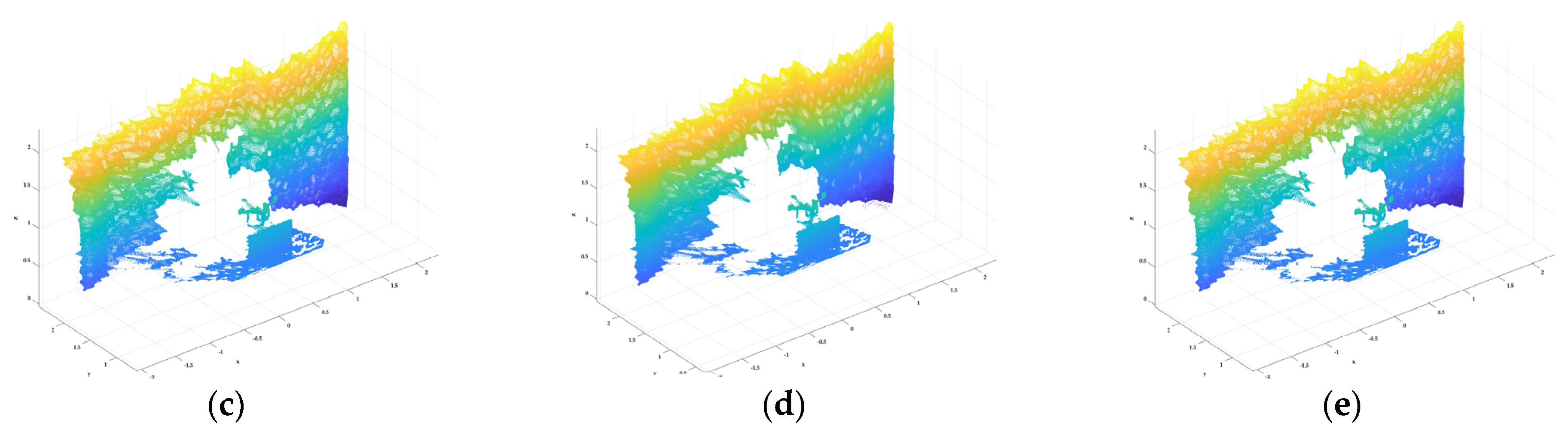
Figure 6.
Denoising effect of fractional integral denoising and median filtering. (a) RGB image (dataset number 00033); (b) deep pseudo-colour map (dataset number 00033); (c) noise-free point cloud image; (d) point cloud image with added noise, PSNR = 46.58 dB; (e) point cloud image filtered by fractional integral denoising (ν = −0.3, PSNR = 52.509 dB); and (f) point cloud of the depth image after median filtering and denoising (PSNR = 39.141 dB).

Figure 7.
Fractional denoising effect with different orders of the fractional integral (PSNR, dB).

Figure 8.
Optimal fractional integral filter denoising order.

Figure 9.
Denoising effects of fractional integral denoising and median filtering. (a) RGB image (dataset number 05959); (b) deep pseudo-colour map (dataset number 05989); (c) noise-free point cloud image; (d) point cloud image with added noise, PSNR = 47.307 dB; (e) point cloud image filtered by fractional integral denoising (ν = −0.3, PSNR = 52.992 dB); and (f) point cloud of the depth image after median filtering and denoising (PSNR = 37.480 dB).


Figure 10.
Denoising effects of fractional integral denoising and median filtering. (a) RGB image (dataset number 03236); (b) deep pseudo-colour map (dataset number 03236); (c) no noise point cloud image added; (d) point cloud image with added noise, PSNR = 47.599 dB; (e) point cloud image filtered by the fractional integral denoising (ν = −0.3, PSNR = 52.070 dB); (f) point cloud of the depth image after median filtering and denoising (PSNR = 36.107 dB).

Figure 11.
Denoising effects of fractional integral denoising and median filtering. (a) RGB image (dataset number 03528); (b) deep pseudo-colour map (dataset number 03528); (c) noise-free point cloud image; (d) point cloud image with added noise, PSNR = 50.094 dB; (e) point cloud image filtered by fractional integral denoising (ν = −0.4, PSNR = 53.847 dB); and (f) point cloud of the depth image after median filtering and denoising (PSNR = 37.855 dB).

Figure 12.
Denoising effects of fractional integral denoising and median filtering. (a) RGB image (dataset number 02350); (b) deep pseudo-colour map (dataset number 02350); (c) noise-free point cloud image; (d) point cloud image with added noise, PSNR = 54.611 dB; (e) point cloud image filtered by fractional integral denoising (ν = −0.3, PSNR = 57.391 dB); and (f) point cloud of the depth image after median filtering and denoising (PSNR = 36.309 dB).

Figure 13.
Denoising effects of fractional integral denoising and median filtering. (a) RGB image (dataset number 09860); (b) deep pseudo-colour map (dataset number 09860); (c) noise-free point cloud image; (d) point cloud image with added noise, PSNR = 43.457 dB; (e) point cloud image filtered by fractional integral denoising (ν = −0.4, PSNR = 51.289 dB); and (f) point cloud of the depth image after median filtering and denoising (PSNR = 37.326 dB).

Figure 14.
Denoising effects of the fractional integral denoising and median filtering. (a) RGB image (dataset number 08343); (b) deep pseudo-colour map (dataset number 08343); (c) noise-free point cloud image; (d) point cloud image with added noise, PSNR = 46.934 dB; (e) point cloud image filtered by fractional integral denoising (ν = −0.3, PSNR = 50.870 dB); and (f) point cloud of the depth image after median filtering and denoising (PSNR = 32.112 dB).

Figure 15.
Denoising effects of fractional integral denoising and median filtering. (a) RGB image; (b) deep pseudo-colour map; (c) noise-free point cloud image; (d) point cloud image of the depth image filtered by the fractional integral denoising (ν = −0.3, PSNR = 53.764 dB); and (e) point cloud of the depth image after median filtering and denoising (PSNR = 34.708 dB).


Table 1.
Fractional integral filter denoising results.
| Dataset Number | V(Best) | PSNR(Best) | PSNR | PSNR |
|---|---|---|---|---|
| Fractional Integral Denoising (dB) | Noise (dB) | Median Filter Denoising (dB) | ||
| 05989 | −0.3 | 52.992 | 47.307 | 37.480 |
| 03236 | −0.3 | 52.070 | 47.599 | 36.107 |
| 03528 | −0.4 | 53.847 | 50.094 | 37.855 |
| 02350 | −0.3 | 57.391 | 54.611 | 36.309 |
| 09860 | −0.4 | 51.289 | 43.457 | 37.326 |
| 08343 | −0.3 | 50.870 | 46.934 | 32.112 |
Table 2.
Fractional integral denoising operator filtering results.
| Data Set | PSNR (dB) | Valid Point (Normal) | Valid Point (After Statistical Outlier Removal) |
|---|---|---|---|
| Original depth image | 100.00 | 854,500 | 831,126 |
| Median filter denoising | 34.708 | 855,799 | 831,126 |
| Fractional integral ) | 53.764 | 854,575 | 841,309 |
Publisher’s Note: MDPI stays neutral with regard to jurisdictional claims in published maps and institutional affiliations. |
© 2022 by the authors. Licensee MDPI, Basel, Switzerland. This article is an open access article distributed under the terms and conditions of the Creative Commons Attribution (CC BY) license (https://creativecommons.org/licenses/by/4.0/).
Share and Cite
MDPI and ACS Style
Huang, T.; Wang, C.; Liu, X. Depth Image Denoising Algorithm Based on Fractional Calculus. Electronics 2022, 11, 1910. https://doi.org/10.3390/electronics11121910
AMA Style
Huang T, Wang C, Liu X. Depth Image Denoising Algorithm Based on Fractional Calculus. Electronics. 2022; 11(12):1910. https://doi.org/10.3390/electronics11121910
Chicago/Turabian StyleHuang, Tingsheng, Chunyang Wang, and Xuelian Liu. 2022. "Depth Image Denoising Algorithm Based on Fractional Calculus" Electronics 11, no. 12: 1910. https://doi.org/10.3390/electronics11121910
Note that from the first issue of 2016, this journal uses article numbers instead of page numbers. See further details here.