
Routing Algorithms Simulation for Self-Aware SDN


Institute of Theoretical and Applied Informatics, Polish Academy of Sciences (ITAI PAS), Baltycka 5, 44-100 Gliwice, Poland
*
Author to whom correspondence should be addressed.
Electronics 2022, 11(1), 104; https://doi.org/10.3390/electronics11010104
Submission received: 30 November 2021
/
Revised: 23 December 2021
/
Accepted: 27 December 2021
/
Published: 29 December 2021
(This article belongs to the Special Issue Artificial Intelligence Driven Software-Defined Networking (SDN) Technologies for Next Generation Networks)
Abstract
:This paper presents a self-aware network approach with cognitive packets, with a routing engine based on random neural networks. The simulation study, performed using a custom simulator extension of OmNeT++, compares RNN routing with other routing methods. The performance results of RNN-based routing, combined with the distributed nature of its operation inaccessible to other presented methods, demonstrate the advantages of introducing neural networks as a decision-making mechanism in selecting network paths. This work also confirms the usefulness of the simulator for SDN networks with cognitive packets and various routing algorithms, including RNN-based routing engines.
1. Introduction
Modern computer networks are used to transmit increasing amounts of data. Optimal routing in backbone networks is a constant challenge due to the tension between the increasingly ubiquitous IoT, with more and more devices being connected to the network via high-bandwidth 5G protocols, and users’ demands for higher bandwidth and low latency. The goal is to provide not only high quality of service—high bandwidth and low latency—but also security, privacy, and low power consumption.
Developers of new hardware and algorithmic solutions are working to meet the needs of network users. New network architectures include software-defined networks (SDNs) [1,2]. SDNs significantly extend the available network management capabilities. A central controller enables the collection of data on the state of the entire network and making decisions about its configuration, particularly about paths for particular network flows, on a basis broader than that available to a single node. It is also much easier to collect data external to the network, for example, the energy consumption of individual nodes or the state of network security monitored by specialized anomaly-detection units.
In particular, SDNs allow all previously known routing methods to be used, although they require new implementation. Meanwhile, the knowledge of the state of the entire network allows us to think about implementing new routing methods that use aggregated data in a way that was previously unavailable in order to search for optimal packet routes in the network.
These advantages were exploited during the construction of the prototype SerIoT network [3]. The basic criterion during its design was the introduction of security-by-design mechanisms for Internet of Things networks. To realize this, random neural networks (RNNs), proposed by Gelenbe [4], were employed to make routing path decisions. The input data for the neural network was collected by cognitive packets (also an invention of Gelenbe) [5]. The effectiveness of these networks was confirmed in multi-criteria routing, where the most important issue was to increase the security level of the network. Other criteria included QoS, energy efficiency and user-defined rules used to construct privacy policies [6,7].
The research and development work required the involvement of specific hardware resources. The use of a specific configuration of laboratory network nodes gave sufficient possibilities at the stage of testing the prototype, however—as is usual in such cases—the flexibility of network configuration, modification and extension of its topology, etc. are limited by the laboratory’s capabilities. Therefore, we decided to create a CPN-over-SDN network simulator.
The simulation study we performed was aimed at proving the usability of the simulator for research on routing in SDN networks and at verification of the conditions under which RNN-based routing proves its value. The SDN environment, providing a central controller, allows the implementation of both routing based on distributed algorithms as well as methods using whole network data. The study compared distributed, random neural networks (RNNs)-based routing with graph-based methods which are typical for SDNs. Both approaches are enhanced with cognitive packets—the mechanism used for gathering QoS data, missing in the standard SDN. Despite the number of publications concerning the various applications of RNNs in routing (in addition to those mentioned above, the following may be referenced [8,9] and others), a decision engine based on this class of neural networks is not often compared to other routing methods. Shortest path search algorithms in a graph seem to be the optimal solution for SDNs with a central controller. It is to be expected that a distributed solution would perform less well, but as a fair comparison has never been made, the level of difference between these two different approaches to the network pathfinding problem remained unknown. A relatively simple simulation study on a network larger than the configurations available in the laboratory was expected to give at least an approximate answer.
An additional motivation was the possibility of creating a research tool—a discrete event simulator—which will be useful not only for this study but will also make it possible to explore further solutions for networks controlled by neural-network-based engines.
The content of the article is as follows. In Section 2, after a brief overview of different approaches to routing issues in IoT, we describe the theoretical basis of the mechanisms and methods used in the simulator. In Section 2.1 we describe the RNN and the decision engine based on it; in Section 2.2 we present the mechanism of cognitive packets, complementing the data needed by the routing engine and missing in the SDN controller; in Section 2.3 we describe the learning process based on the available (also thanks to CPN) data; while in Section 2.4 we refer to the methods that we take as a reference in the centralized network architecture. Section 3 is devoted to basic information related to the construction of the simulator. Section 4 describes the experiments performed, while their results are presented synthetically in Section 5. Section 6 presents a brief summary and conclusions.
2. Routing Methods for SDN
Routing in the modern Internet is based on the BGP protocol [10], which bases its operation on information exchanged between routers. It reacts very well and quickly to changes in the connection topology, but it is difficult to naturally incorporate parameters for optimization, such as QoS or energy efficiency. While it is unlikely that significant changes will occur in the traditional Internet due to well-established standards, new segments of the network services market—mobile networks and Internet of Things (IoT)—are developing rapidly, and with their development, a number of different solutions in the area of routing are also being proposed.
There are many proposals to develop mobile networks—one of many is the architecture proposed by the 4WARD project [11], which allows for a high degree of flexibility by covering both existing and new protocol paradigms. Specific solutions of their own are also proposed by developers of the Internet of Things. These include adaptations of existing solutions, such as 6LoWPAN standardized by IETF [12] and its extension RPL [13]. Some routing protocol proposals, such as TRAIL [14], take into account various security threats. Fully distributed examples include LOADng [15] and CORLP. The former follows a reactive approach—it establishes routes only if there are packets to transport. However, it suffers from control traffic overhead. The latter is in turn a protocol dedicated to Advanced Metering Infrastructure (AMI) networks, wireless but not mobile. A completely different approach based on game theory, taking into account both security elements and energy consumption in IoT, is shown in turn in [16]. The work [17] is also of interest, and presents a heuristic search for an optimal solution considering two metrics: energy consumption and traffic delay.
This short overview by no means exhausts the subject of new routing techniques in networks. However, it shows that the authors approached the problem in different ways, proposing solutions which are both universal and dedicated to specific technologies, with these solutions being an extension of existing algorithms or completely new proposals. It is interesting that many of the works cited used event-driven simulation (EDS) techniques for their research, often using the OmNeT++ simulator (ns is also used very often). This paper is in turn a simulation evaluation of a method that is rather typical for machine learning (ML).
2.1. Software Defined Networks
A software-defined network (SDN) is a network architecture in which the control layer is separate from the packet transmission devices (routers, switches). An SDN involves a separate device—the controller—that decides how individual packets travel through the network. SDN switches (also called forwarders) do not implement any decision-making mechanism. They receive rules from the controller, according to which they should treat incoming packets. The rules state that packets meeting certain conditions—related to source and destination addresses, protocol, etc.—are forwarded to the appropriate forwarder output port. The packet can also be broadcast (copied to all output ports) or forwarded to the controller. Usually, the default rule for unknown packets is to send the packet to the controller so that the controller can decide how to forward the packet. The decision is propagated to the forwarders in the form of subsequent rules, so that subsequent packets are forwarded without involving the controller.
This architecture offers a wide range of configuration possibilities. It is possible to apply various criteria for deciding which paths to take in the network, appropriate to the current situation. It is possible to migrate previously used routing algorithms to the controller, as they are easier to implement and test in the central controller. It is also possible to use completely new algorithms, taking advantage of the fact that the state of the entire network is known to the controller. A typical SDN controller (e.g., [18,19,20]) implements some basic routing method that ensures that a connection is established, but does not in any way guarantee the quality of the connection. On the other hand, SDN controllers are equipped with an API that allows them to implement their own arbitrary routing decision methods. Implementing new routing algorithms is thus relatively easy, and SDN is an excellent tool for experimenting with routing.
RNN were first used to control routing in a computer network some twenty years ago [5,21]. However, the approach used in the computer network, using cognitive packets to collect quality-of-service data, and the presence of neural networks at each node was incompatible with the standard TCP/IP protocol stack. Only later implementations of cognitive packets encapsulated in UDP frames circumvented this limitation.
Continuing the work described in [6], carried out on physical nodes in the laboratory of IITiS PAN, we decided to create an event-driven simulator that allows the modification of the applied algorithms more freely and which will give much more flexibility in creating network topologies. Studies of topologies larger than a few nodes will become possible.
2.2. Decision Engine
The RNN module follows the idea of distributed control, originally presented by Gelenbe in [5], where every node was accompanied by an instance of RNN. In the SDN implementations, the RNNs are moved to the single location of the SDN controller, still preserving the distributed logical architecture of RNNs interconnected in a way reflecting the physical topology.
Computer networks transport data in packets. In SDN, a collection of packets with the same source and destination address is referred to as a flow. The goal of the decision engine for each flow is to find a path having lowest latency, which means the best quality of service (QoS). Latency is calculated by summing up the delays d on particular links l belonging to the path. Thus, for given flow f going along path P, the latency is:
The value of represents the goal function necessary for the training and operation of the RNN. As the aim of the decision engine is to lower the value of , we need a reward function which increases as the quality of the answer improves. We introduce the reward function R:
We assume that all the values which influence the value of , and hence the value of , are taken with measurements made by cognitive packets. Every cognitive packet contains data that allows the cognitive network map to update the latency on each link visited by the given CP. The decision engine after the application of RL algorithms is able to answer which output port the user packet should take in every subsequent node to reach its destination in the shortest time possible.
2.3. Cognitive Packets
Cognitive packets (CPs, sometimes referred to as smart packets) are control packets or frames designed to carry network parameters and other management information. Their original use was to carry timestamps of visits to each node along the path to provide RNN-based routers with QoS (link delay) data. The CP wandered from one node to another, both following the paths defined for the user data packets and wandering completely or partially at random in search of new paths with better parameters, unknown to the neural network [22]. The flow of packets via the node is presented in Figure 1. The packet, incoming from another node, follows the rules stored in a switching table stored in the node. If the node address is different from the CP destination, the current timestamp is added to the CP payload, and the packet is passed to the next node, according to the rules set by the controller and stored in the switching table. If the node address is equal to the CP destination, the packet (after the timestamp is added) goes to the controller, passing the link delays data to the routing engine in the controller and enabling it to update its outcome.
The rule set in the switching table has its timeout or living time. After this time has elapsed, the rule is removed. This, when the next packet arrives, gives the opportunity for the node to ask the controller for a new rule, updated according to the current state of the CNM.
2.4. Learning Process
The RL algorithm first updates the value of the threshold . In the k-th step, represents the value of in step .
The larger the value of , the better the network is doing.
The RNN for a given node is “recursive”, as shown in Figure 2. This means that each neuron is connected to all others. In this way, we allow competition between neurons representing different output ports from a given node. The RL algorithm [23] then calculates a set of RNN connection weights as follows.
The single RNN, corresponding to a single network node , consists of N neurons, where N is the number of out ports for the node . Each out port is associated with a neuron i, and its state is “the probability of excitation” . The weights of the connections between neurons are and , where . The theory of RNN [23] says that:
where represents the total firing rate of neuron i, and the values and are respectively:
The view of neuron i and its neighbors is depicted in Figure 3. is the arrival rate of the excitatory spikes to neuron i, and is the arrival rate of the inhibitory spikes. In the initial state the rate parameters are set making the all weight values equal and all the neurons an excitation probability of . The state represents the situation of equal choice among all out ports in the node.
RL, depending of the value of threshold , updates the weights following the rules:
After the calculation of new weights, they are normalized, dividing every by the sum of all weights in the RNN. The final step is to compute all the values from Equation (4).
The RNN answers are now translated into the SDN rules and sent to every network node to create a switching table. As mentioned above, every output of every node has a neuron corresponding to it. The output i of choice is the one having the highest of all output neurons in the node. Starting from the first node, the controller goes to the next node linked to the output, and by repeating this procedure in every node it is able to complete the path and set appropriate rules in the SDN switches.
To avoid unnecessary “flickering” of paths, or very frequent changes thanks to minimal differences in goal function value between the alternative paths for a given flow, the controller changes the path for the flow f only if the “new” path is better than the “old” path —at least by path change threshold, , in terms of the value of . The path change is effective if or , and the typical value of in experiments varied between 1% and 10%.
This way, all the computations remain in the controller machine, and the SDN switches do not need to have any significant computing power. This is another advantage of the SDN approach compared to the “classic” RNN algorithm.
For the purposes of this study, the decision engine takes into account latency only. The implementation, however, enables the introduction of a more complex goal function . The architecture of the SDN-with-RNN solution, reflected in simulation, is depicted in Figure 4.
2.5. Other Methods
The data gathered with cognitive packets can be used by an alternative decision method. The centralized architecture of the SDN allows for comparison of the RNN decision engine with the classic graph approach. However, we must bear in mind that while the neural network method can also be successfully applied in a distributed architecture, and SDN is only a platform that facilitates its implementation, graph methods require a central point where data from the entire network are collected, and their distribution is impossible. This simulator uses a graph representation in the form of neighborhood lists. The simple approach is to use only the unweighted network graph. A more reasonable method assumes that the weights of individual branches come from cognitive packets informing about the delay in individual links—branches of the graph (the average of the last three measurements on each link). For the data collected in this way, the classical Dijkstra’s shortest path algorithm [25] is applied.
3. SDN-SAN Simulator
The OMNeT++ 4.2 [26] simulator, the Inet 2.0 library (implementation of network elements and protocols) and the OpenFlow protocol SDN library [27] were used as a basis for in-simulator RNN-based routing engine implementation.
To create the SDN-SAN simulator we extended the source code of the OMNeT++ OpenFlow library with the required mechanisms. First, we added cognitive packets generation and handling to simulate the behavior of a real SAN with cognitive packets. Every network node simulated SDN forwarder was accompanied by a cognitive packet agent. The construction of CPs was similar to the real CPs implemented in [28] or [29]. Every CP contained timestamps gathered in the visited nodes, which—along with nodes’ id—gave a clear image of network delays on each particular link. The CP at the end of its road along the SDN network was sent to the SDN controller, filling the cognitive network map with latency data. The Figure 5, Figure 6 and Figure 7 present some of OmNET++ model views.
A server named SD was connected to each switch, and two processes were running on it (udpApp[0] and udpApp[1]). The first one sent cognitive packets (collecting information about the delay on links), the second one was a source of user data packets, transferring data between servers. Thus, the second process corresponded to a simple client connected to the node. We assumed that all links had comparable bandwidth (150 Mbps was assumed in the models).
In the prototype implementation of the real system, we used Open vSwitch as packet for-warder according to SDN rules and CP agent process to handle incoming and generate new cognitive packets. The CP agent was connected to the internal (local) port of Open vSwitch. The simulator architecture described above maintained exactly the same logic.
4. Parameters of RNN Routing Algorithm
The RNN algorithm (implemented in Java due to the ONOS controller) has parameters that can be tuned to improve its performance. To improve the simulation results in the RNN algorithm, the following changes were made:
- 1
- The parameter responsible for taking into account historical values when calculating the reward/penalty for the neural network was reduced from 0.1 to 0.00001 in order to speed up the response to rapidly changing conditions in the network.
- 2
- Threshold of a delay change, after which flow changes occur—this parameter was changed from 10% of the average evaluation (or timeout) of paths in networks to 1%. This means that much less gain in delay caused the change of the path (and the changes were more frequent).
- 3
- The depth of propagation of change information in the graph was increased from 1 (only the best paths were informed and rewarded) to −1, that is, all interesting paths (i.e., containing an updated link) were rewarded/punished. This also increased the speed of response to a change in the network.
- 4
- The buffer of the number of stored previous paths (found by RNN earlier) was reduced from all to a limited size of 10 per source–target pair.
The RNN algorithm with these parameters is henceforth referenced to as RNN+.
5. Simulation Experiments
This report presents the results of simulation studies of SDN-type networks described above, aimed at comparison of three routing algorithms:
- Dijkstra’s simple shortest path algorithm.
- Dijkstra’s algorithm, with edges of the graph weighted with the delays found by CP on the particular links.
- RNN with RL distributed algorithm.
The experiment concerned a hypothetical IoT network, covering a certain area with sensors. The node of the network was represented by an IoT sensor hub, collecting data from a number of sensors, connected to the hub by wire or wirelessly (the connectivity between the sensors and the hub was not simulated). The amount of data from the sensors could change over time. An example to illustrate this model is a network of seismographic sensors distributed over a certain area. They send heartbeat signals at regular intervals and additional data when they detect shocks. Sensor hubs are connected to each other by a cable network. Each hub also acts as an SDN switch—in practice, this means that two separate devices—hub and SDN switch—are contained in one housing, and this is how it was modeled in the experiment. SDN switches were connected via Ethernet.
The topology used for tests is presented in Figure 8. The results are the packet delay times for the specified paths using the above algorithms.
5.1. Cognitive Packets
We consideredfour algorithms (methods) for sending cognitive packets:
- 1
- Each node (SD) sends a cognitive packet to every other node.
- 2
- Each node sends a packet to one node drawn according to a uniform distribution.
- 3
- Each node sends a packet to its neighbor nodes (nodes to which a direct link exists).
- 4
- Node i sends a packet to node i + k, with an initial delay equal to dT/n where n is the number of initial nodes, with a constant delay dT depending on the load k increasing by 1 in each dT cycle.
In order to avoid the situation that all packets are sent simultaneously which could severely overload the network, Lists 1 and 2 assume that the time between consecutive sent COG packets is random with an exponential distribution and a mean value dT.
5.2. Experiment Parameters
All models used the topology form Figure 8. Each sender (sensor hub) sent UDP packets of size 1000 B as user packets. All nodes had a fixed packet processing time, giving them the throughput at the level of 32 Mb/s, which can be considered typical for low-performance, battery-operated devices of the Raspberry Pi class.
The cognitive packets were sent at a fixed interval to the node (List 4 above, ). These assumptions translate to the following OmNeT++ simulation parameters:
udpApp[*].messageLength = 1000B
open_flow_switch*.serviceTime = 0.00025s
sd*.udpApp[0].sendInterval = 0.1s;*.ofa_switch.flow_timeout = 0.33s;
6. Comparison of Routing Algorithms
The algorithms examined were as follows:
- 1
- Simple shortest path (Dijkstra) algorithm with no weights of the graph edges, referred to as DA.
- 2
- Shortest path with weights, where the weight of the graph edge was equal to delay on the corresponding link, referred to as DW.
- 3
- Basic RNN decision engine, referred to as RNN.
- 4
- RNN decision engine with tuned parameters, referred to as RNN+.
The DA (List 1) corresponds to basic standard solutions included in some SDN controllers (e.g., ONOS [18]). This method is topology-based, and uses no QoS data, as they are not present in the controller as standard.
The DW (List 2) utilizes link latency data gathered by cognitive packets. It is still the shortest path method but applied to a graph with weighted edges. The latency is used directly as the weight of the graph edge, and the algorithms looks for the lowest value.
The RNN (List 3) engine used was the same as in previous real testbed experiments (e.g., [6,30]). The experiments denoted as RNN used the same parameter set as in the lab experiment.
The RNN+ experiments (List 4) were performed with RNN with another set of parameters, namely:
- 1
- The value of in Formula (3) was decreased from 0.1 to 0.00001.
- 2
- The path change threshold was changed from 10% to 1%.
These changes accelerated the response of the neural network to changes in network conditions. As it turned out during the tests, parameters suitable under the conditions of the laboratory real network were sub-optimal in the simulated network.
The experiment performed to show the differences between algorithms as well as simulator features was performed in the topology presented in Figure 9. The experiment scenario assumed that the background traffic would flow between pairs of nodes, so that all nodes were involved in sending and receiving packets. Packets were sent at an average rate of 1 packet/0.0025 s (0.4 Mbps) and exponential distribution of inter-sending time. The traffic from node 2 to node 11 was observed. Additionally, after 2 s of simulated time, the traffic between nodes 4 and 9 was started with an average rate of 1 packet/0.000625 s (1.6 Mbps), and from 3 to 10 with 1 packet/0.00125 s (0.8 Mbps), also having exponential distribution of inter-sending time. This traffic resulted in increased delays for packets traveling from 2 to 11 and the need for the routing engine to search for new paths.
6.1. Measurements
Figure 10, Figure 11, Figure 12 and Figure 13 present latency on the path 2–11 with different routing methods.
The table in Figure 14 lists the path changes when the most active RNN+ routing engine was employed look for the path. Please note that the average delays shown in the right-hand column were measured when the path was changed to the next one, and they were not the basis for the change decision, but the times measured by the cognitive packets. However, the heuristic nature of the method based on neural networks is evident—you can see the frequent changes of paths caused by the fact that each change of path modified the conditions in the whole network, affecting other flows, which in turn had a feedback effect on the delays in the path of the observed flow from 2 to 11.
Average delay times for all the flows during the whole experiment for particular methods were as follows:
- 1
- DA: 0.00231 s.
- 2
- DW: 0.00284 s.
- 3
- RNN: 0.20006 s.
- 4
- RNN+: 0.00595 s.
The graph in Figure 15 presents the latency for each flow.
6.2. Overview of the Results
In the graphs of packet delay in the network we see a different behavior of the graph methods, the RNN-based engine without tuned parameters and the routing version RNN+, with improved parameters. Both the delay graph for a specific path from node 2 to node 11 and the averaged packet delay in the network indicate that the use of the data we obtained using a centralized network architecture yielded very good results. In the tested scenario, despite some expectations, the introduction of cognitive packets did not significantly improve the results when switching from DA to DW method. A comparison of the graph as well as the total average delay times indicates that RNN was clearly inferior to the other methods. However, the engine parameters affected the performance significantly. In the RNN version, the response was later and weaker than in RNN+, and although the maximum delays were lower, the average delay was significantly higher for RNN than RNN+. This is due to the fast and efficient response of the routing engine in the RNN+ version.
7. Conclusions
This paper compared the performance of routing based on Gelenbe’s neural network RNN with routing based on graph approaches. Such a comparison is possible in SDN networks, where a central controller is able to collect data about the state of the entire network.
As expected, the simulation results confirmed that graph algorithms are fast and efficient because the representation of a computational network using a graph is natural. Reflecting the cost of choosing a given network path in the form of a graph branch weights allows optimal solutions to be found, and the speed of the algorithms allows them to be used almost continuously.
However, the method based on RNNs has an undeniable advantage—it can operate in a distributed manner. The results of the routing algorithm (i.e., path selection decisions obtained using RNNs) would be the same (and of similar order of performance) if we abandoned the central data collection point and each network was placed in a node whose decisions it is responsible for.
The results of these simulation studies show that RNNs, with an appropriate choice of parameters for their operation, can produce results of comparable quality to graph algorithms, but the questions on how to select these parameters remain unanswered in the general case. However, this should be considered as an important premise for conducting further research on the application of artificial intelligence methods in the control of computer networks.
This report also demonstrates the usefulness of simulation methods (e.g., discrete event simulator) for testing algorithms controlling traffic in computer networks, including neural networks.
Author Contributions
Conceptualization, methodology and experiment design, M.P.N.; software, P.P. All authors have read and agreed to the published version of the manuscript.
Funding
This research was funded by European Commission Horizon 2020 research and innovation programme within “IoTAC” project, grant agreement No. 952684.
Conflicts of Interest
The authors declare no conflict of interest.
References
- McKeown, N.; Anderson, T.; Balakrishnan, H.; Parulkar, G.; Peterson, L.; Rexford, J.; Shenker, S.; Turner, J. OpenFlow: Enabling innovation in campus networks. ACM SIGCOMM Comput. Commun. Rev. 2008, 38, 69–74. [Google Scholar] [CrossRef]
- Gude, N.; Koponen, T.; Pettit, J.; Pfaff, B.; Casado, M.; McKeown, N.; Shenker, S. NOX: Towards an operating system for networks. ACM SIGCOMM Comput. Commun. Rev. 2008, 38, 105–110. [Google Scholar] [CrossRef]
- Domańska, J.; Gelenbe, E.; Czachórski, T.; Drosou, A.; Tzovaras, D. Research and innovation action for the security of the internet of things: The SerIoT project. Commun. Comput. Inf. Sci. 2018, 821, 101–118. [Google Scholar] [CrossRef] [Green Version]
- Gelenbe, E. Random neural networks with negative and positive signals and product form solution. Neural Comput. 1989, 1, 502–510. [Google Scholar] [CrossRef]
- Gelenbe, E.; Xu, Z.; Seref, E. Cognitive Packet Networks. In Proceedings of the ICTAI ’99—11th IEEE International Conference on Tools with Artificial Intelligence, Chicago, IL, USA, 9–11 November 1999; IEEE Computer Society: Washington, DC, USA, 1999; p. 47. [Google Scholar]
- Gelenbe, E.; Domańska, J.; Fröhlich, P.; Nowak, M.P.; Nowak, S. Self-Aware Networks That Optimize Security, QoS, and Energy. Proc. IEEE 2020, 108, 1150–1167. [Google Scholar] [CrossRef]
- Gelenbe, E.; Fröhlich, P.; Nowak, M.; Papadopoulos, S.; Protogerou, A.; Drosou, A.; Tzovaras, D. IoT Network Attack Detection and Mitigation. In Proceedings of the 9th Mediterranean Conference on Embedded Computing, MECO 2020, Budva, Montenegro, 8–11 June 2020; IEEE: Piscataway, NJ, USA, 2020; pp. 1–6. [Google Scholar] [CrossRef]
- Wang, L. Online Work Distribution to Clouds. In Proceedings of the 2016 IEEE 24th International Symposium on Modeling, Analysis and Simulation of Computer and Telecommunication Systems (MASCOTS), London, UK, 19–21 September 2016; pp. 295–300. [Google Scholar] [CrossRef] [Green Version]
- Francois, F.; Gelenbe, E. Optimizing Secure SDN-Enabled Inter-Data Centre Overlay Networks through Cognitive Routing. In Proceedings of the 2016 IEEE 24th International Symposium on Modeling, Analysis and Simulation of Computer and Telecommunication Systems (MASCOTS), London, UK, 19–21 September 2016; pp. 283–288. [Google Scholar] [CrossRef]
- Rekhter, Y.; Hares, S.; Li, T. A Border Gateway Protocol 4 (BGP-4) (RFC 4271); IETF: Fremont, CA, USA, 2006. [Google Scholar]
- Singh, A.; Nass, C.; Timm-Giel, A.; Schefczik, P.; Roessler, H.; Scharf, M. Generic Connectivity Architecture for Mobility and Multipath Flow Management in the Future Internet. In Mobile Networks and Management, Second International ICST Conference, MONAMI 2010, Santander, Spain, 22–24 September 2010; Springer: Berlin/Heidelberg, Germany, 2010. [Google Scholar] [CrossRef]
- Alexander, R.; Brandt, A.; Vasseur, J.; Hui, J.; Pister, K.; Thubert, P.; Levis, P.; Struik, R.; Kelsey, R.; Winter, T. RPL: IPv6 Routing Protocol for Low-Power and Lossy Networks (RFC 6550); IETF: Fremont, CA, USA, 2012. [Google Scholar]
- Le, A.; Loo, J.; Lasebae, A.; Vinel, A.; Chen, Y.; Chai, M. The Impact of Rank Attack on Network Topology of Routing Protocol for Low-Power and Lossy Networks. IEEE Sens. J. 2013, 13, 3685–3692. [Google Scholar] [CrossRef]
- Perrey, H.; Landsmann, M.; Ugus, O.; Schmidt, T.C.; Wählisch, M. TRAIL: Topology authentication in RPL. arXiv 2013, arXiv:1312.0984. [Google Scholar]
- Clausen, T.; Yi, J.; Herberg, U. Lightweight On-demand Ad hoc Distance-vector Routing—Next Generation (LOADng): Protocol, extension, and applicability. Comput. Netw. 2017, 126, 125–140. [Google Scholar] [CrossRef]
- Duan, J.; Gao, D.; Yang, D.; Foh, C.H.; Chen, H.H. An Energy-Aware Trust Derivation Scheme With Game Theoretic Approach in Wireless Sensor Networks for IoT Applications. IEEE Internet Things J. 2014, 1, 58–69. [Google Scholar] [CrossRef]
- Zhou, B.; Zhang, F.; Wang, L.; Hou, C.; Anta, A.F.; Vasilakos, A.V.; Wang, Y.; Wu, J.; Liu, Z. HDEER: A Distributed Routing Scheme for Energy-Efficient Networking. IEEE J. Sel. Areas Commun. 2016, 34, 1713–1727. [Google Scholar] [CrossRef]
- Open Network Operating System (ONOS®). The Open Networking Foundation. Available online: https://opennetworking.org/onos/ (accessed on 15 April 2021).
- RYU Project Team. RYU SDN Framework. Using OpenFlow 1.3; Ryu SDN Framework Community, 2014. Available online: https://book.ryu-sdn.org/en/Ryubook.pdf (accessed on 20 September 2021).
- The Linux Foundation. OpenDaylight Project; 2021. Available online: https://www.opendaylight.org/ (accessed on 10 November 2021).
- Gelenbe, E.; Lent, R.; Xu, Z. Design and performance of cognitive packet networks. Perform. Eval. 2001, 46, 155–176. [Google Scholar] [CrossRef]
- Gelenbe, E. Cognitive Packet Network. U.S. Patent 6804201 B1, 12 October 2004. [Google Scholar]
- Gelenbe, E. Learning in the Recurrent Random Neural Network. Neural Comput. 1993, 5, 154–164. [Google Scholar] [CrossRef]
- Gelenbe, E. The Random Neural Network and Its Application to Cognitive Packet Networks. The Lecture at IARAI, Vienna. 18 February 2021. Available online: https://www.iarai.ac.at/events/the-random-neural-network-and-its-application-to-cognitive-packet-networks/ (accessed on 8 December 2021).
- Dijkstra, E.W. A note on two problems in connexion with graphs. Numer. Math. 1959, 1, 269–271. [Google Scholar] [CrossRef] [Green Version]
- Varga, A.; Hornig, R. An overview of the OMNeT++ simulation environment. In Proceedings of the SimuTools, Marseille, France, 3–7 March 2008. [Google Scholar]
- Klein, D.; Jarsche, M. An OpenFlow Extension for the OMNeT++ INET Framework. In Proceedings of the 6th International ICST Conference on Simulation Tools and Techniques, Cannes, France, 5–7 March 2013. [Google Scholar]
- Nowak, M.; Nowak, S.; Domanska, J. Cognitive Routing for Improvement of IoT Security. In Proceedings of the IEEE International Conference on Fog Computing ICFC, Prague, Czech Republic, 24–26 June 2019. [Google Scholar] [CrossRef]
- Fröhlich, P.; Gelenbe, E. Optimal fog services placement in SDN IoT network using Random Neural Networks and Cognitive Network Map. In Artificial Intelligence and Soft Computing, Proceedings of the ICAISC, Zakopane, Poland, 12–14 October 2020; Lecture Notes in Computer Science; Springer: Cham, Switzerland, 2020; Volume 12415, pp. 78–89. [Google Scholar] [CrossRef]
- Fröhlich, P.; Gelenbe, E.; Nowak, M.P. Smart SDN management of fog services. In Proceedings of the 2020 Global Internet of Things Summit (GIoTS), Dublin, Ireland, 3 June 2020; IEEE: Piscataway, NJ, USA, 2020; pp. 1–6. [Google Scholar]
Figure 1.
The flow of user and cognitive packets in the networks.

Figure 2.
Architecture of an RNN for single flow in a six-output node [24].
Figure 2.
Architecture of an RNN for single flow in a six-output node [24].
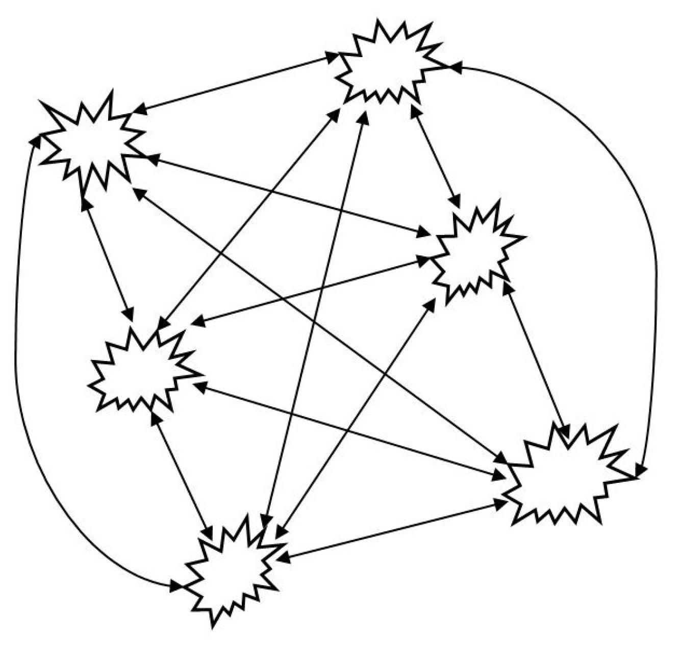
Figure 3.
An RNN neuron and its neighbors.

Figure 4.
Internal architecture of the SDN solution with RNN.

Figure 5.
Main module: network Scenario14nodes.

Figure 6.
Module of class standardHost.

Figure 7.
Module of class ofSwitch.

Figure 8.
Topology of the experimental network.

Figure 9.
Configuration of the experiment.

Figure 10.
Delays on the path 2–11: DA method.

Figure 11.
Delays on the path 2–11: DW method.

Figure 12.
Delays on the path 2–11: RNN method.

Figure 13.
Delays on the path 2–11: RNN+ method.

Figure 14.
Switching of the paths during the experiment presented in Figure 13.
Figure 14.
Switching of the paths during the experiment presented in Figure 13.

Figure 15.
Delays on particular paths (ending node shown on the X axis).

Publisher’s Note: MDPI stays neutral with regard to jurisdictional claims in published maps and institutional affiliations. |
© 2021 by the authors. Licensee MDPI, Basel, Switzerland. This article is an open access article distributed under the terms and conditions of the Creative Commons Attribution (CC BY) license (https://creativecommons.org/licenses/by/4.0/).
Share and Cite
MDPI and ACS Style
Nowak, M.P.; Pecka, P. Routing Algorithms Simulation for Self-Aware SDN. Electronics 2022, 11, 104. https://doi.org/10.3390/electronics11010104
AMA Style
Nowak MP, Pecka P. Routing Algorithms Simulation for Self-Aware SDN. Electronics. 2022; 11(1):104. https://doi.org/10.3390/electronics11010104
Chicago/Turabian StyleNowak, Mateusz P., and Piotr Pecka. 2022. "Routing Algorithms Simulation for Self-Aware SDN" Electronics 11, no. 1: 104. https://doi.org/10.3390/electronics11010104
Note that from the first issue of 2016, this journal uses article numbers instead of page numbers. See further details here.