Machine Learning (ML) Based Thermal Management for Cooling of Electronics Chips by Utilizing Thermal Energy Storage (TES) in Packaging That Leverages Phase Change Materials (PCM)

Abstract

Miniaturization of electronics devices is often limited by the concomitant high heat fluxes (cooling load) and maldistribution of temperature profiles (hot spots). Thermal energy storage (TES) platforms providing supplemental cooling can be a cost-effective solution, that often leverages phase change materials (PCM). Although salt hydrates provide higher storage capacities and power ratings (as compared to that of the organic PCMs), they suffer from reliability issues (e.g., supercooling). “Cold Finger Technique (CFT)” can obviate supercooling by maintaining a small mass fraction of the PCM in a solid state for enabling spontaneous nucleation. Optimization of CFT necessitates real-time forecasting of the transient values of the melt-fraction. In this study, the artificial neural network (ANN) is explored for real-time prediction of the time remaining to reach a target value of melt-fraction based on the prior history of the spatial distribution of the surface temperature transients. Two different approaches were explored for training the ANN model, using: (1) transient PCM-temperature data; or (2) transient surface-temperature data. When deployed in a heat sink that leverages PCM-based passive thermal management systems for cooling electronic chips and packages, this maverick approach (using the second method) affords cheaper costs, better sustainability, higher reliability, and resilience. The error in prediction varies during the melting process. During the final stages of the melting cycle, the errors in the predicted values are ~5% of the total time-scale of the PCM melting experiments.

1. Introduction

Rapid miniaturization of electronics device elements has accelerated their performance and efficacy in commercial products. This has led to higher rates of heat dissipation, which is a limiting factor in maximizing their performance. Semiconductor reliability, product lifetime, and performance diminish at elevated operating temperatures. Maldistribution of temperature (“hot spots”) can lead to early and catastrophic failures also. Higher junction temperatures due to the hot spots result in a shortened lifespan of a semiconductor device. In fact, the chances of failure increase exponentially, if a local area on a chip heats up beyond the specified temperature [1]. This result is based on the widely known Black’s equation [2]. Moreover, integration—a direct consequence of miniaturization—has resulted in non-uniform heat flux generation. The progression of the state of the art of semiconductor technologies has largely followed the famous Moore’s law [3]—which simply states that the number of transistors on a microchip will double every two years or so. However, the doubling rate has started to falter in recent times, primarily due to the failure of the packaging industries in meeting the heat dissipation requirements [4]. Removal of high heat flux at appropriate temperatures is a constant challenge faced by the electronics industry. Researchers have considered varied approaches for electronics cooling over the years [5,6]. Hence, to extract maximum efficacy from these innovations —which are accruing from progressive miniaturization of electronics devices and packages into increasingly smaller form factors—better thermal management strategies and paradigms are needed to address the higher cooling loads (and for mitigating the localized transient hot spots).

1.1. PCMs for Electronics Cooling

Traditional cooling techniques typically consist of external air-cooled heat sinks and are inadequate for satisfying the cooling loads from modern electronics. Emerging technologies include (i) Heat pipes; (ii) Heat pumps; (iii) Microchannels; (iv) Spray cooling; (v) Phase change material (PCM) based cooling; (vi) Free cooling; and (vii) Thermoelectric cooling [7]. A number of studies on these techniques have enabled the rank ordering of their efficacies [8,9,10]. Among these, passive cooling (e.g., leveraging PCMs) have garnered significant attention in recent times due to their cost-effectiveness and simplicity. Desirable properties of these PCMs (e.g., high latent heat, narrow operating temperature envelope, high specific heat, and small volume expansion on melting) translate into compact form factors of the electronics chips and packages. A numerical study exploring the novel design of a heat sink utilizing hollow aluminum pin fins filled with PCM showed that a small mass of PCM could effectively stabilize the microprocessor temperatures [11]. An experimental study on the cooling of a personal digital assistant (PDA) using n-eicosane as a PCM for thermal energy storage (TES) showed that this architecture stabilized the junction temperatures and the effectiveness of such a heat storage unit depends on the amount of PCM used [12]. PCMs can be used for thermal control of electronics devices that have intermittent duty cycles, such as for mobile phones, digital video cameras, wearable computers, and video-gaming chips. The thermal resistance of the device and the power rating of the PCM mass (for charging and discharging cycles) are the critical design parameters in this type of passive system [13]. A PCM based heat sink (where the PCM is deposited in the cavities of the sink) placed on a plastic quad flat package mounted on a printed circuit board was shown to have improved cooling performance as compared to that of the case without PCM, especially at high power levels (q), that is, q exceeding 2 W [14]. Another study reported that for a fixed volume of PCM in the heat sink: the operation time (time required for the heat sink to achieve a target temperature) was enhanced significantly, where the degree of enhancement was elevated at progressively higher power levels [15]. It has been established that combining a PCM-based heat sink with forced air convection provides a superior strategy in reducing (or damping) the peak temperatures than that of a traditional air-cooled heat sink without PCM. Moreover, the higher TES capacity of the PCM (due to higher latent heat values) increases the time needed to reach the peak temperature. For effective thermal management of electronics, it is desirable that PCMs should possess the following characteristics and properties—(i) appropriate and narrow band of the phase transition temperature, (ii) low volume expansion coefficients (and during phase change), (iii) elevated thermo-physical properties (e.g., thermal conductivity, latent heat, and specific heat capacity values), (iv) material compatibility (non-corrosive) and chemical stability (especially for repeated melting and freezing), (v) low/no supercooling during freezing, (vi) low cost and (vii) minimal environmental footprint [16]. All of these criteria can be seldom met in one candidate PCM exclusively, and therefore, often a trade-off must be made for choosing the appropriate PCM for a given application.

1.2. Supercooling in PCMs

PCMs can be categorized as: (1) organic, (2) inorganic, and (3) eutectics. Examples of organic PCMs include paraffin, fats, and fatty acid-based derivatives. Popular inorganic PCMs include-salt hydrates such as (LiNO₃ · 3(H₂O)) and metallics such as Gallium. Eutectics are often realized by utilizing a mixture of two or more PCMs that provide congruent melting and freezing points. Salt hydrates have a higher volumetric energy storage capacity (40–125 (kWh/m³)) than paraffins (40–60 (kWh/m³)) due to their high densities [17]. Higher thermal conductivity and thermal diffusivity values of inorganic PCMs also enable higher power ratings of the TES platforms. So, in systems where volume is a constraint, salt hydrates can be a better option. However, salt hydrates undergo incongruent melting and often require large supercooling to initiate nucleation. Supercooling is the phenomenon where solidification is achieved only when the PCM temperature is significantly lower than the thermodynamic phase transition temperature. At the fusion temperature, the rate of nucleation is very low. This limits the efficacy of a PCM heat sink—as the latent heat is not released.

Methods to address supercooling can be categorized into passive and dynamic techniques. The addition of nucleating agents is a widely studied passive technique to mitigate supercooling. Using Borax (e.g., at a mass fraction of 1.9%) as a nucleating agent reduced the degree of supercooling for thickened Glauber’s salt from 15 °C to 3~4 °C [18]. Supercooling in sodium acetate trihydrate (SAT) was entirely obviated upon the addition of aluminum nitride (AlN) nanoparticles at a mass fraction of 5% along with carboxyl methyl cellulose (CMC) as a thickening agent at a mass fraction of 4% [19]. Supercooling in SAT can also be reduced by adding silver nanoparticles and was reported to vary as a function of the concentration of the nanoparticles [20]. Similarly, copper hydroxyl nitrate hydrate (CHNH) catalyst enhances nucleation in lithium nitrate trihydrate (LNT). Models suggest that the similarity of the lattice structures of both the salt and the catalyst (or nucleators) determine their effectiveness at mitigating supercooling [21]. Zinc hydroxyl nitrate and zinc oxide nucleators were observed to reduce the supercooling in zinc nitrate trihydrate by 8.8 °C to 8.2 °C, respectively [22]. The effect of various nucleating agents on the degree of supercooling in salt hydrates has been extensively reviewed in multiple reports in the literature [23,24].

In contrast to the heterogeneous seeding techniques, the “cold finger technique” (CFT) is an example of a homogenous nucleation technique where a small mass fraction of the salt hydrate crystals are maintained in a solid phase (un-melted) in contact with the liquid phase, thus aiding spontaneous nucleation when freezing is initiated. A localized spot (or tiny mass fraction) can be maintained in the solid phase by adding extra insulation or exerting localized pressure. Another way to implement the cold finger technique is to halt the melting process of the PCM just prior to complete melting. For instance, the heat source could be removed when the PCM is 85% melted, leaving 15% un-melted (in order to promote spontaneous nucleation during the freezing cycle). However, the enhanced reliability in CFT is achieved at the expense of reduced energy storage capacity.

Combining CFT with a forecasting technique (for predicting the time required to reach a target melt-fraction) can successfully mitigate reliability issues by obviating supercooling while maximizing the energy storage capacity (and to some extent the power rating) of the TES platform utilizing inorganic PCMs. For a TES application requiring repeated thermocycling (i.e., repeated consecutive cycles of melting and freezing), CFT was demonstrated to be effective in reducing the degree of supercooling in LNT (from ~10 °C) to less than 1 °C (e.g., in the range of 0.5–1 °C). The authors demonstrated that using the CFT technique the LNT samples survived thermocycling tests that exceeded 800 cycles of repeated incomplete melting and complete solidification [25].

Motivated by the goal of improving the effectiveness of inorganic PCMs incorporated into TES platforms that can be deployed for electronics chip cooling applications, in this study, the efficacy of deep learning is explored for enhancing the energy storage capacity for CFT by forecasting the time required to reach a target melt-fraction (say, 85% or 99%). In this study, a graduated measuring cylinder was filled with PCM and an electrically powered heater was mounted at the bottom of the cylinder to melt the PCM. Thermocouples were mounted within the body of the PCM as well as on the surface of the measuring cylinder at specific locations. A digital data acquisition system was used to record the temperature transients from the thermocouples. The temperature data were fed to an ANN model with the goal of performing real-time predictions for the time required to reach a target melt-fraction (e.g., 85%). Hence, artificial neural network (ANN) models were developed in this study for real-time prediction of the time remaining to reach a predefined (or target) melt-fraction at any instant during the experiments as the PCM melts. This study was performed to contrast the efficacy of two different approaches utilizing the same ANN model:

(1)

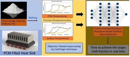
Using temperature data from sensors immersed within the body of the PCM at locations corresponding to meniscus levels of the liquid coinciding with specific values of melt-fraction of the PCM (i.e., transient PCM-temperature data for training of the ANN model); and

(2)

Using temperature data from sensors mounted on the surface of the cylindrical container at locations corresponding to meniscus levels of the liquid coinciding with specific values of melt-fraction of the PCM (i.e., transient surface-temperature data for training of the ANN model).

The efficacy of these two approaches is compared for different values of the electrical power input to the heater (that is mounted at the bottom of the cylindrical container). The errors in the predictions from the ANN model (compared to the actual values recorded in the experiments) are explored for different sets of training data obtained from these experiments.

2. Artificial Neural Network Principles

Artificial neural networks are capable of fitting complex, non-linear mappings between inputs and outputs [26]. An ANN can be defined as a parallel distributed processing system capable of learning from experiences [27]. ANNs are built to construct relationships between parameters without detailed knowledge about the system. The most basic kind of ANN is the fully connected multilayer perceptron (MLP) model. In such networks, the neuron is the fundamental processor of information. These neurons (also referred to as “nodes”) are arranged in progressive layers. In the case of a fully connected MLP, a neuron receives and processes the input from the neurons in the previous layer into an output. A neuron can be mathematically characterized by: (i) bias (b); and (ii) activation function (f). Each synaptic connection is associated with a weight (w). Inside every node, the activation function acts on the weighted inputs from the previous layer. Let the subscript n denote the serial number of the layer. The input vector to the layer can be represented by a_n. The relationship between the output (the input to a_n+1) is depicted in Equation (1) below:

$$a_{n+1}=f\left(w^T{a}_n+b\right)$$

(1)

Developing an ANN model involves training, validation, and testing stages. The input data and the output (predictions) can be divided into three sets, one for each stage. The weights and biases are randomly initialized. The output (i.e., the set of predicted value(s) from the ANN model) is obtained using these random parameters. A cost function then quantifies the degree of disagreement (or error) between the generated (predicted) output and the actual (true) output, thus going through the validation step. This obtained error is propagated backward from the output to the input layer by adjusting the weights and biases. A gradient descent algorithm is applied to modify the biases and weights to optimize (minimize) the cost function. This feedforward and backpropagation process continues until the target error (or target gradient) is achieved or the number of passes (epochs) reaches a specified value. A typical example of the cost function is the “sum of squared errors” (SSE) on the validation dataset depicted in (2) where p is the true value and p’ is the value predicted by the ANN model. Also, N denotes the size of the test set. The third stage involves testing the efficacy of the ANN on the test dataset, which was not encountered by the ANN during the training or the validation stage.

$$\mathrm{SSE}={\displaystyle \sum }_{i=1}^N{\left(p-p^{\prime }\right)}^2$$

(2)

The efficacy of a neural network for improving the reliability of a TES platform has been previously studied by the authors of this paper [28]. For electronics cooling applications, PCM heat sinks are an emerging solution. During intermittent operation of electronic devices–a heat sink filled with PCM can limit the peak value of the local temperature transients by rapid melting (faster discharging cycle) and release the heat when the device is idle (slow period of freezing, i.e., slower charging cycle). During thermocycling of PCM, the power rating is typically higher during the charging cycle (i.e., during melting, since it is dominated by free-convection heat transfer) and the power rating is lower during the discharging cycle (i.e., during freezing, since it is dominated by conduction heat transfer and convection is almost negligible) [25]. Thus, this strategy helps with extending the time required to reach the peak temperature of the heat sink, especially under critical load conditions [29].

As mentioned before, in this study, the prediction errors from the ANN model that is trained using transient surface-temperature data are compared with the same ANN model that is trained using temperature transients recorded by thermocouples immersed within the volume of the PCM. Measurements of surface temperature transients are preferable for electronics packages (filled with PCMs) due to their simplicity, low cost, enhanced reliability, as well as ease of manufacturing and fabrication. Such a capability can facilitate lower failure rates while also providing ease of access for maintenance operations and repair jobs. Forecasting strategies based on transient surface-temperature data also enable retrofitting of existing electronics devices with capabilities for real-time predictions using ANN models (e.g., the time remaining for reaching a target melt-fraction of PCMs that are filled inside the electronics package). These capabilities do not typically accrue from strategies involving measurement of temperature transients from sensors that are immersed within the volume of PCM, that is, from temperature sensors mounted inside the electronics package (instead of the surface-mounted temperature sensors). Hence, this study demonstrates the efficacy of ANN models for electronics chip cooling applications and can be used in conjunction with PCM-filled heat sinks to improve their reliability for thermal management applications (e.g., in data centers).

3. Experimental Apparatus and Procedure

Thermocycling experiments were conducted in this study to obtain a dataset consisting of temperature transients and the corresponding values of melt-fraction. PureTemp 29^TM is chosen as the candidate PCM in these experiments. The salient properties of Pure Temp29^TM are listed in

Table 1. Salient Properties of PureTemp29 [30].

Property	Value
Enthalpy of Phase Change	202 (J/g)
Heat Capacity of Solid	1.77 (J/(g °C))
Heat Capacity of Liquid	1.94 (J/(g °C))
Density of Solid	0.94 (g/mL)
Density of Liquid	0.85 (g/mL)
Conductivity of liquid	0.15 (W/(m °C))
Conductivity of solid	0.25 (W/(m °C))

. The data from these experiments were used for training an ANN model. The goals of these experiments and numerical simulations were focused on deploying the ANN model for real-time prediction of the time required to reach a target value of melt-fraction (e.g., 85%). The errors in the predictions (compared to experimental data) were obtained from this study with the goal of identifying the ANN model that yields the best performance.

A solid sample of PCM was heated in a graduated measuring cylinder (with a total volume of 50 mL) and with a least count of 1 mL. The experiments were performed until the PCM was melted completely. Broadly, the apparatus consists of four components: (i) the graduated measuring cylinder; (ii) K-type thermocouples; (iii) heater coil; and (iv) Data acquisition system.

The thermocouples were mounted at specific locations—both within the volume of the cylinder, as well as on the outside surface of the cylinder. These locations were determined strategically in order to measure the temperatures at particular heights (from the bottom) and along the axis of the cylinder. The vertical heights were chosen strategically to correspond to the level of the liquid meniscus of the melted PCM for a pre-determined value of melt-fraction.

The heater assembly is composed of a Nichrome wire (coil) connected to a DC power supply. The coil is placed at the bottom of the cylinder for melting the PCM for a fixed value of input power. The ends of the coil are connected to a DC supply by means of insulted connecting wires. Such a configuration means that when the liquid meniscus is at 0 mL marking (i.e., there is no melting), the PCM is at a 0% melt-fraction. Whereas, when the liquid meniscus is at the 50 mL marking, the PCM is at a 100% melt-fraction. The thermocouples are placed at particular locations (within the volume of the PCM) and along the axis of the cylinder corresponding to 30%, 60%, 85%, 90%, 95%, and 99% melt-fraction. On the outer surface of the measuring cylinder, the surface-mounted thermocouples are located at heights corresponding to 30%, 60%, 90%, and 99% melt-fraction. In addition to these sets, another thermocouple is located at a distance of 1 cm above the 50 mL mark on the outside surface of the measuring cylinder, that is, at a distance of 1 cm above the height of the meniscus corresponding to a 100% melt-fraction. Thermal paste (Omegabond^TM) is used as a glue to mount the thermocouples on the outside surface of the measuring cylinder. The thermocouples are calibrated in the temperature range of 20 °C to 40 °C. The calibration step involves the measurement of the steady-state temperature of each thermocouple when placed in a water bath and the temperature measurements were recorded by an automated digital data acquisition system for a period of 1 min. The calibration was performed for fixed temperature values (of the water bath) corresponding to 20 °C, 25 °C, 30 °C, 35 °C, and 40 °C. The calibration was performed using a NIST calibrated mercury thermometer with a least count of 0.1 °C. The resultant calibration error (instrument/ bias error and statistical error) was estimated to be less than ±0.1 °C with a 68% statistical confidence (i.e., within one standard deviation of the average value).

3.1. Volume Calibration Experiments

The location of the thermocouples along the axis of the cylinder and its outer surface is based on the particular location of the liquid meniscus of the PCM (as it melts progressively) corresponding to chosen and specific values of melt-fraction of the PCM. A series of volume-calibration experiments were performed in the measuring cylinder (before performing the PCM experiments) in order to determine the height corresponding to a particular value of the volume of the liquid phase. This was performed by filling the measuring cylinder with a fixed quantity of water and noting the level of the liquid meniscus in the measuring cylinder. With the heater assembly and the thermocouple positioning apparatus inside the cylinder, water is poured in 5 mL aliquots. The water level rise is recorded until the water reaches the 50 mL mark. Due to the volume occupied by the apparatus inside, the volume level shown by the cylinder is higher than the actual volume of water in it. Using the densities of the solid and liquid PCM phases, the cylinder markings corresponding to the chosen melt-fractions are determined. Interestingly, there exists a maximum value of the melt-fraction (less than 100%) such that the thermocouple at that point remains inside the PCM mass throughout the experiment. This occurs due to PCM volume shrinkage. Upon solidification of the PCM, the thermocouples mounted at locations corresponding to higher values of melt-fraction (which are initially submerged in the liquid PCM) are then exposed to air (instead of being submerged in the solidified mass of PCM) since the air-PCM interface recedes upon complete solidification of the PCM. In this experiment, thermocouples were mounted at locations corresponding to melt-fraction exceeding 95% and therefore, would not be immersed in the PCM during the entirety of the experiments. Hence, initially at the beginning of the melt-cycle, these thermocouples would be exposed to air (and will record the temperature of the surrounding air). However, towards the final stages of the melt-cycle (when the melt-fraction exceeds 95%), these thermocouples will be submerged in the liquid PCM and would record the temperature of the liquid phase of the PCM.

3.2. Data Acquisition (DAQ) System

A digital data acquisition system (NI SCXI 1303 board with the NI SCXI 1000 chassis, from National Instruments Inc., Austin, TX, USA) was used for recording the transient temperature data from the thermocouples. The data acquisition process was automated using Labview^TM software (from National Instruments Inc.). The photograph of the experimental setup is shown in Figure 1. Figure 2 schematically depicts the different components of the experimental apparatus. A plastic tube was inserted into the measuring cylinder (prior to filling it with PCM). The plastic tube was used for mounting the thermocouples and for the purpose of placing the beaded ends of the thermocouples at specific locations precisely along the vertical direction. The lower end of the plastic tube was sealed to prevent PCM from seeping in, and the thermocouple wires emerged out of the upper end of the plastic tube. The cylinder is filled with liquid PCM up to the 50 mL mark and allowed to solidify under ambient conditions.

Digital images of the whole volume of PCM within the measuring cylinder were captured every 60 s during the melting experiments in order to monitor the rise of the liquid-solid interface along the vertical direction. An infra-red (I.R.) camera was used to capture I.R. images intermittently at specific intervals of time. The I.R. images were used to monitor the temperature distribution and ascertain temperature uniformity within different parts of the experimental apparatus. Representative I.R. images are shown in Figure 3 at different points in time. Using the apparatus, melting experiments were performed by setting the heater voltage at a constant value. The thermocouple and the visual data (digital images and IR images) were recorded until complete melting of the PCM was achieved.

Experiments were performed for three sets of heater input voltages—2.8 V (1.6 W), 2.6 V (1.4 W), and 2.3 V (1.08 W). Each experiment was conducted twice to verify the repeatability of the experimental data. The transient temperature data recorded by the thermocouples are plotted using a line graph. Figure 4 shows the transient temperature profile recorded by the thermocouples that were mounted within the mass of PCM (“transient PCM-temperature data”). Figure 5 shows the transient temperature profile recorded by thermocouples mounted on the surface of the measuring cylinder (“transient surface-temperature data”). In these plots, the abscissa denotes the elapsed time in seconds [s].

The goal of this study was to predict in real-time (i.e., at any instant during the melting process)—the time remaining to attain an 85% melt-fraction. In deep learning terms, the “time to reach 85% melt-fraction” is the label. This label is obtained by subtracting the time recorded corresponding to each temperature measurement (consisting of the following set: [T₃₀, T₆₀, T₈₅, T₉₀, T₉₅, T₉₉, T’₃₀, T’₆₀, T’₉₀, T’₉₉, T_ambient]) from the time when melt-fraction of 85% is attained. The target value of an 85% melt-fraction is achieved when the melt front hits the particular thermocouple inside the PCM mass (indicated by the sudden rise in temperature recorded by that particular thermocouple). This point is indicated by the temperature profile of that thermocouple (Figure 4). The temperature curve begins to plateau after a sharp increase. The time stamp on this point serves our purpose for generating the labels.

A Multilayer Perceptron (MLP) Network is devised with three input nodes. Figure 6 shows the topology of the neural network. The PCM temperatures, marked as: T₃₀, T₆₀, and T₉₀; constitute the three inputs. A non-dimensional quantity, referred to as reduced time, is formulated. Nondimensionalizing the time parameter allows us to train the ANN using one experimental dataset and predict for another case. This reduced time, τ, is obtained by taking the ratio of the elapsed time to the time when the target value (85% melt-fraction) is achieved. It follows that the nondimensional form of the label is then the complementary value of τ (i.e., obtained by subtracting τ from unity and is denoted by τ’). Figure 7 depicts the plot of temperatures as a function of nondimensional time (τ) and was obtained after implementing the aforementioned steps (summarized in this paragraph). The three inputs to the ANN are (as mentioned before): T₃₀, T₆₀, and T₉₀. The output of the ANN is τ’. When exploring the performance of an ANN trained on surface temperatures, T₃₀, T₆₀, T₉₀ get replaced by surface temperatures T’₃₀, T’₆₀, and T’₉₀, respectively.

The MLP model (i.e., the artificial neural network/ANN model) is trained using τ’ as the label and the three temperature inputs (recorded by the experiment for a particular power input). The training process is based on the well-known back-propagation algorithm which modifies the weights and biases of a node as it iterates through the dataset. The training process is stopped by using the “early stopping” approach. In other words, when the MSE does not improve substantially upon further iterations, the training process is halted. The neural network in this study is composed of three hidden layers and each layer has 512 nodes. The Rectified Linear Unit (ReLU) activation function is used in the network nodes. The cost function for training purposes is the Mean Squared Error (MSE). ADAM optimizer is deployed as the gradient descent algorithm. The predictions are generated for all six combinations of training/prediction by utilizing the three datasets.

4. Results and Discussion

Table 2. Time to reach specific values of melt-fraction for different values of power input to the heater.

Heater Voltage (V)	Time to Reach 85% Melt-Fraction (s)	Time to Reach 90% Melt-Fraction (s)	Time to Reach 100% Melt-Fraction (s)
2.3 V	12,017	13,670	15,658
2.6 V	11,817	12,729	13,157
2.8 V	8768	9888	10,518

lists the time taken to reach various melt-fractions for the three datasets. The experiments performed for 2.3 V input to the heater correspond to a current of 0.47 A and a power input of 1.08 W. When the heater input voltage is 2.6 V, the heater draws a current of 0.54 A and a power input of 1.4 W. For 2.8 V input, the current and power inputs are 0.58 A and 1.6 W, respectively. We observe that the times needed to attain an 85% melt-fraction for the 2.3 V and 2.6 V experiments are quite similar. This is attributed to the ambient temperature effects. For the 2.3 V experiment, the average ambient temperature is observed to be 22.8 °C (standard deviation = 0.2 °C) whereas, for the 2.6 V experiment, the average recorded ambient temperature is 22.3 °C (standard deviation = 0.2 °C). The repeatability of the experiments can be established by plotting temperature transients recorded by a thermocouple, for example, T₃₀ against non-dimensional time (where the total time spans from 0 to 100% melt). As an example, Figure 8, Figure 9 and Figure 10 show, the repeatability of the 2.8 V experiment. The initial temperatures of the solid PCM at the beginning of the two instances of the 2.8 V experiment are different (due to different ambient conditions) causing the deviations observed in Figure 8, Figure 9 and Figure 10. The heat lost from the apparatus (due to free convection and radiation phenomena) is also influenced by the ambient temperature. Additional plots of the experimental data for the different power inputs are provided in Appendix A.

4.1. Performance of the ANN Trained on PCM Temperatures

The three datasets (2.3 V, 2.6 V, and 2.8 V input) are used in all possible permutations of training and prediction sets. For instance, the temperature transients obtained from the thermocouples immersed in the PCM for 2.6 V input are used to train the neural network. This ANN is then used to predict the time remaining to reach 85% melting for the 2.8 V input condition (and the errors in the predicted values are calculated from the experimental data for the 2.8 V input condition). For a graphical representation, the predictions are depicted on a scatter plot for any combination of the training and prediction datasets. For instance, using the 2.6 V dataset for training and deploying the ANN (to obtain the predictions on the 2.8 V input condition) then yields the scatter plot in Figure 11. The non-dimensional plot can be dimensionalized by multiplying the predicted τ’ values by the time-duration to attain 85% melting (from Table 2) and is depicted in Figure 12. The solid red line (y = x curve) serves as a reference for deviations of the predictions from the actual (“true” experimental) values. The dotted lines mark the point when the PCM reaches 30% and 60% melt-fractions (which are registered by individual thermocouples mounted at each of those specific locations). On the non-dimensional scatter plot (e.g., Figure 11), the green dotted line represents the point when the melt front reaches the respective thermocouple on the training set whereas the blue dotted line denotes the same on the prediction set. The prediction error is formulated as the difference between the predicted value and the actual value of time (in seconds). A low error is desired particularly at the final stages, that is, when the PCM is about to reach a melt-fraction of 85% so that the melting cycle can be halted in time in a real-life application of this method. For a training/prediction combination of 2.6 V/2.8 V, the average absolute error in the final 1800 s (0.5 h) before reaching an 85% melt-fraction is about 3 min (167 s), which is a minute fraction (~2%) of the total cycle time (8768 s).

As another combination, the ANN model is trained on the 2.3 V set and deployed to predict on the 2.8 V dataset. The results for the predictions from the ANN model are plotted in Figure 13. At approximately 3000 s prior to reaching an 85% melt-fraction, the prediction error is observed to peak to a value of ~1000 s. However, the average absolute error in the last 1800 s (before reaching an 85% melt-fraction) is 331 s, which corresponds to a minute fraction (~4%) also. With the training/prediction combination of 2.8 V/2.3 V, the same metric is 653 s which amounts to ~5% of the total time to reach an 85% melt-fraction (of the 2.3 V set).

Table 3. Average absolute error in the final 1800 s (prior to attaining a melt-fraction of 85%) for different training/prediction data-set combinations using transient PCM-temperature data.

	Prediction Set
		2.3 V	2.6 V	2.8 V
Training Set	2.3 V		190 s	331 s
	2.6 V	423 s		167 s
	2.8 V	653 s	233 s

summarizes the prediction errors for all combinations of training/prediction datasets. This ANN method, applied on a simple experimental apparatus, yields prediction errors that are less than 10 min., for a forecasting point that is 3 h ahead of reaching the target melt-fraction of 85%. Hence, the efficacy of the method is established, and this demonstrated the feasibility of the ANN model (or MLP model), as well as the computational and experimental techniques that were deployed in this study.

4.2. Performance of the ANN Trained on Surface Temperatures

The profiles of transient surface-temperature data recorded in these experiments were similar to that of the temperature transients recorded within the mass of PCM (as shown in Figure 5). Another ANN model is trained using the transient surface-temperature data recorded in the same experiments: and are denoted as T’₃₀, T’₆₀, and T’₉₀ (as the inputs) instead of the PCM temperatures. The topology of the neural network and the τ’ labels are the same. Scatter plots and errors are obtained as outlined in the previous section. Figure 14 shows the scatter plot for 2.6 V and 2.8 V datasets for training and prediction respectively. The surface thermocouples are exposed to higher levels of noise from the ambient environment (as compared to that of the thermocouples immersed in the mass of PCM). As a result, the profile of the transient surface-temperature data is not as smooth (as compared to that of the transient PCM-temperature data). Hence, the fluctuations in the predicted values are observed to be higher for the ANN models trained using the transient surface-temperature data. Despite this impediment, the average error in the last 1800 s is 502 s (~6% of the total cycle time).

The ANN model that was trained using the transient surface-temperature data obtained from the experiments performed for 2.3 V input was then deployed to obtain predictions for the experiments using 2.8 V input. The results are plotted in Figure 15. In this case, the deviation is minimized as compared to that of Figure 13. A summary of the average absolute errors is listed in

Table 4. Average absolute error in the final 1800 s (prior to attaining a melt-fraction of 85%) for different training/prediction data-set combinations using transient surface-temperature data.

	Prediction Set
		2.3 V	2.6 V	2.8 V
Training Set	2.3 V		201 s	206 s
	2.6 V	589 s		502 s
	2.8 V	279 s	447 s

. Despite being higher (compared to the magnitude of the errors listed in Table 3), the magnitudes of the errors listed in Table 4 are still less than 600 s (10 min.), when the real-time forecasting is performed 1800 s (30 min.) prior to reaching the target melt-fraction of 85%. Comparison of the tabulated errors (between Table 3 and Table 4), shows that the transient surface-temperature data do not conclusively provide a better strategy for training the ANN models (instead of leveraging the transient PCM-temperature data), specifically for improving the accuracy of the predictions during the final stages of melt-cycle and close to the target values of the melt-fraction. However, the errors are still appreciably low. From a functional standpoint, we can feed surface temperatures to an ANN to predict the time to reach a predefined melt-fraction. It may be noted that underprediction of the time is desirable (it is more reliable)—since over-prediction of the time can cause complete melting of the PCM in the TES, which is a catastrophic failure (since the PCM would then need to be supercooled to achieve nucleation and freezing). For electronics with intermittent operating cycles (i.e., fluctuating duty cycles), this method can be used to leverage the benefits accrued for deploying salt hydrates as PCMs in TES platforms (higher reliability and energy storage capacities with augmented power ratings) while also obviating supercooling.

At lower melt-fractions, the prediction errors are lower for the ANN model trained using transient surface-temperature data than that of the ANN model trained using PCM temperature data (for target melt-fraction of 85%). Line graphs are utilized to compare the error in prediction for the two input categories—transient surface-temperature data and transient PCM-temperature data. For instance, as shown in Figure 16 (training set: 2.3 V, prediction set: 2.6 V), for abscissa values in the range of 6000 s to 10,000 s; lower values of absolute error are obtained for the predictions from the ANN model trained using transient surface-temperature data, compared to that of the ANN model trained using PCM temperature data. This trend is again evident in Figure 17 (training set: 2.8 V, prediction set: 2.6 V) for abscissa values ranging between 6500 s and 9000 s. For yet another case, as shown in Figure 18 (training set: 2.6 V, prediction set: 2.3 V) for abscissa values ranging from 7000 s to 12,000 s; the predictions from the ANN model (that was trained using transient surface-temperature data) yield lower magnitudes of the absolute error than those of the ANN model trained using the PCM temperature data. Similar trends are evident in the plots shown in Figure 19, Figure 20 and Figure 21.

Also, it may be noted that for ANN model predictions using transient PCM-temperature data, the errors in the predictions are lower when the input power (or input voltage) for the training data is closer to the input voltage of the prediction set. In other words, when 2.6 V data are used for training, the error in the predictions is lower for 2.8 V input conditions than that of the 2.3 V input conditions. Similarly, when the 2.8 V data are used for training, the error in the predictions is lower for 2.6 V input conditions than that of the 2.3 V input conditions.

In contrast, it may be noted that for ANN model predictions using transient surface-temperature data, the error in the predictions is lower when the input power (or input voltage) for the training data is starkly different compared to the input voltage of the prediction set. In other words, when 2.8 V data are used for training, the error in the predictions is lower for 2.3 V input conditions than that of the 2.6 V input conditions. Similarly, when the 2.3 V data are used for training, the error in the predictions is lower for 2.8 V input conditions than that of the 2.6 V input conditions. This contrast in the prediction capabilities of the ANN model can be attributed to the nature of the training data set itself. On closer observation, it may be noticed that the transient surface-temperature data have more acute levels of fluctuations (owing to exposure to free convection to the ambient air) than that of the transient PCM temperature data (owing to the high thermal energy storage capacity locally within the PCM-that tends to damp out any acute temperature fluctuations due to their higher thermal-inertia/thermal-inductance and thermal-capacitance).

Also, it is worth noting that for ANN model predictions using transient surface-temperature data, the error in the predictions is lower when the input power (or input voltage) for the training data is 2.3 V. In contrast, for ANN model predictions using transient surface-temperature data, the error in the predictions is highest when the input power (or input voltage) for the training data is 2.6 V. Whereas, for ANN model predictions using transient surface-temperature data, the error in the predictions is moderately high when the input power (or input voltage) for the training data is 2.8 V. This anomalous trend can be explained by exploring the nuances of the experimental observations. During the later stages of the melting cycle, especially at higher power input conditions (2.6 V and 2.8 V experiments)–it was observed that the rate of propagation of the melt front was fast enough that it partially lifted the solid mass of PCM above it by a minute amount. This was akin to a hydraulic ram actuation caused by the volumetric expansion due to solid-to-liquid phase change as the liquid PCM has a lower density than that of the solid phase (and the solid mass of PCM above the melted liquid-phase acts like a hermetically sealed piston preventing the liquid PCM from leaking up). At which point the plastic tube embedded in the solid mass of PCM caused an opposing reaction force resulting in restoration of the solid mass of PCM back towards the original position. This caused a ripple effect in the temperature transients that were recorded by both the thermocouples embedded in the PCM and by the thermocouples mounted on the surface of the measuring cylinder (this occurred typically towards the end of the melt-cycle and at high values of melt-fraction when the melt-fraction exceeded ~80%). As a result, the training data set for these cases cause distortions in the parameters defining each neuron in the ANN model (i.e., the weight function, the activation function, and the bias). Consequently, the predictions from these ANN models display high magnitudes of error and are also less reliable (i.e., often cause over-predictions).

In contrast, at lower power input conditions (2.3 V experiments), the melt front propagated very slowly (since the power input was barely in excess of the heat loss from the measuring cylinder by free convection). As a result, the solid mass of PCM was virtually undisturbed in these experiments. As a result, there is less distortion in the parameters defining individual neurons. Consequently, the predictions from the ANN model trained using transient temperature data from the 2.3 V experiments (either for the surface temperature data set or the PCM temperature data set) have better fidelity. Consequently, the magnitude of the error is lower, and the predictions are more reliable (i.e., the results tend to underpredict the time required to reach the target value of 85% melt-fraction) for a major proportion of the melt-cycles.

5. Conclusions

Motivated by the need to improve the performance and reliability of Thermal Energy Storage (TES) platforms utilizing Phase Change Materials (PCMs) this study is aimed at leveraging Machine Learning (ML) techniques for augmenting the efficacy of the Cold-Finger-Technique (CFT) by obviating supercooling phenomena of PCMs. Experiments were performed using digital data acquisition apparatus (including flow visualization by a digital camera, I.R. thermography measurements for verification of temperature uniformity in different segments of the experimental apparatus and measurement of temperature transients using thermocouples that were mounted strategically at specific locations corresponding to the location of the liquid meniscus of the PCM for chosen values of melt-fractions). The experiments were performed for power input values of 1.08 W, 1.4 W, and 1.6 W. This study proves the feasibility of obtaining real-time predictions using Multi-Layer Perceptron (MLP)/Artificial Neural Network (ANN) models for improving the reliability and efficacy of TES platforms that leverage PCMs. This approach, therefore, enables the successful deployment of the “Cold Finger Technique” (CFT) to obviate supercooling. Thus, the storage capacity of the TES is maximized while also enhancing the reliability and resilience of the cooling strategy. This is achieved by deploying the MLP/ANN models for real-time prediction of the time remaining to attain a target (predefined) melt-fraction during the melting cycle. The target value of melt-fraction chosen in this study is 85%. Data sets obtained for a chosen power input condition are used for predicting (and validating) the values for another set of power input conditions.

Two different approaches were explored for training the ANN models: (1) by using transient PCM temperature data; and (2) by using transient surface-temperature data. Lower magnitudes of error in the predicted values were obtained for ANN models trained using transient surface-temperature data corresponding to lower power input conditions (since anomalous temperature transients were minimized at lower power input conditions due to the gradual progression of the PCM upwards into the mass of solid PCM). The predictions were also found to be reliable for a major proportion of the melt-cycle (i.e., the values were underpredicted). On the other hand, anomalous decreases in temperature trends were observed for the temperature transients recorded at higher power input conditions (both for surface temperature and PCM temperature data). This was due to the volumetric expansion of the trapped liquid phase (upon melting from the solid phase), which caused the solid mass of PCM above to be displaced up (followed subsequently by a downward motion of the solid PCM caused by the restoring force of the plastic tube adhering to the solid mass of PCM at the top)—resulting in a sharp decrease in the temperature values recorded by thermocouples that were already submerged in the liquid PCM (and for the surface thermocouples that were mounted at similar heights from the base of the measuring cylinder). Consequently, the parameters for each neuron (e.g., weight function, bias, etc.) in the ANN model were likely to be distorted, thus causing a higher magnitude of errors in the predicted values and the predictions were unreliable (i.e., due to over-predictions) for a major proportion of the melt-cycle.

In contrast, for ANN models trained using transient PCM-temperature data, lower magnitudes of error in the predicted values were obtained when the input power of the training data set was similar to that of the predicted data set. For example, lower magnitudes of error were obtained when the training data set from the 2.6 V experiments were utilized for predicting the temporal values for the 2.8 V experiments. Similarly, lower magnitudes in error were obtained when the training data set from the 2.8 V experiments were utilized for predicting the temporal values for the 2.6 V experiments. In contrast, the magnitudes of error were higher (and the values were over-predicted, i.e., the predictions were unreliable for a major proportion of the melt-cycle) for the 2.3 V experiments when either the data set from 2.6 V or from 2.8 V were utilized for training the ANN model. In general, the accuracy of predictions afforded by ANN models that were trained using transient surface-temperature data was higher in the initial stages of the cycle (however, higher levels of error are observed for these cases in the final stages of the melting cycle). Future directions of this study include implementing these experimental studies and ANN model development on actual (e.g., “commercially off-the-shelf” or “COTS”) electronics chips that leverage PCM-filled heat sinks. Optimization of the neural network parameters also needs to be explored.

Motivated by the potential application of inorganic PCMs in TES (that can be deployed for enhancing the reliability and resilience of thermal management devices), especially in electronics chip cooling platforms, in this study, the efficacy of deploying deep learning is explored for enhancing the energy storage capacity for CFT (without compromising the power rating) by forecasting the time required to reach a target melt-fraction. In these applications, the direct measurement of PCM temperature is often not possible due to packaging-related issues. Measurement of surface-temperature transients is preferable for electronics packages (especially for those that are filled with PCMs) due to their simplicity, low cost, better reliability, as well as ease of manufacturing and fabrication. This strategy can yield lower failure rates while also providing ease of access for maintenance and repair operations. Forecasting strategies based on transient surface-temperature data also enable retrofitting of existing thermal-management platforms in electronics devices thus rendering additional capabilities for real-time predictions using ANN models (e.g., the time remaining for reaching a target melt-fraction of PCMs that are filled inside the electronics package). These capabilities do not typically accrue from strategies involving measurement of temperature transients from sensors that are immersed within the volume of PCM, that is, from temperature sensors mounted inside the electronics package (instead of the surface-mounted temperature sensors). Hence, this study demonstrates the efficacy of ANN models for electronics chip cooling applications and can be used in conjunction with PCM filled heat sinks to improve their reliability for thermal management applications (e.g., in data centers) while also impacting the sustainability of these data-centers by reducing the usage of water (e.g., reducing the demand for chilled water and, in turn, the evaporative losses from the cooling towers), as well as the net power consumption by the data centers. Secondary benefits that accrue from such endeavors include augmented cooling capabilities and enhanced performance of the thermal management platforms, better durability and increased longevity of the computing platforms; since more effective deployment of the thermal management platforms that leverage such real-time predictions capabilities from the ANN models result in better temperature uniformity (i.e., mitigating the hot-spots in the packages of the electronics chips and within the chips themselves).

References

1. Pedram, M.; Nazarian, S. Thermal Modeling, Analysis, and Management in VLSI Circuits: Principles and Methods. Proc. IEEE 2006, 94, 1487–1501. [Google Scholar] [CrossRef] [Green Version]
2. Black, J.R. Electromigration—A brief survey and some recent results. IEEE Trans. Electron Devices 1969, 16, 338–347. [Google Scholar] [CrossRef] [Green Version]
3. Moore, G.E. Cramming More Components Onto Integrated Circuits. Proc. IEEE 1998, 86, 82–85. [Google Scholar] [CrossRef]
4. Waldrop, M. The chips are down for Moore’s law. Nat. News 2016, 530, 144. [Google Scholar] [CrossRef] [Green Version]
5. Markowski, P.M.; Gierczak, M.; Dziedzic, A. Temperature Difference Sensor to Monitor the Temperature Difference in Processor Active Heat Sink Based on Thermopile. Electronics 2021, 10, 1410. [Google Scholar] [CrossRef]
6. Kang, T.; Ye, Y.; Jia, Y.; Kong, Y.; Jiao, B. Enhanced Thermal Management of GaN Power Amplifier Electronics with Micro-Pin Fin Heat Sinks. Electronics 2020, 9, 1778. [Google Scholar] [CrossRef]
7. Murshed, S.M.S.; de Castro, C.N. A critical review of traditional and emerging techniques and fluids for electronics cooling. Renew. Sustain. Energy Rev. 2017, 78, 821–833. [Google Scholar] [CrossRef]
8. Maydanik, Y.; Vershinin, S.; Korukov, M.; Ochterbeck, J. Miniature loop heat pipes-a promising means for cooling electronics. IEEE Trans. Compon. Packag. Technol. 2005, 28, 290–296. [Google Scholar] [CrossRef]
9. Wei, X.; Joshi, Y. Stacked Microchannel Heat Sinks for Liquid Cooling of Microelectronic Components. J. Electron. Packag. 2004, 126, 60–66. [Google Scholar] [CrossRef]
10. Garimella, S.V.; Singhal, V.; Dong, L. On-Chip Thermal Management With Microchannel Heat Sinks and Integrated Micropumps. Proc. IEEE 2006, 94, 1534–1548. [Google Scholar] [CrossRef]
11. Jaworski, M.; Domański, R. A novel design of heat sink with PCM for electronics cooling. In Proceedings of the 10th International Conference on Thermal Energy Storage, Stockton, CA, USA, 31 May–2 June 2006; Volume 31. [Google Scholar]
12. Tan, F.L.; Tso, C.P. Cooling of mobile electronic devices using phase change materials. Appl. Therm. Eng. 2004, 24, 159–169. [Google Scholar] [CrossRef]
13. Kandasamy, R.; Wang, X.-Q.; Mujumdar, A.S. Application of phase change materials in thermal management of electronics. Appl. Therm. Eng. 2007, 27, 2822–2832. [Google Scholar] [CrossRef]
14. Kandasamy, R.; Wang, X.-Q.; Mujumdar, A.S. Transient cooling of electronics using phase change material (PCM)-based heat sinks. Appl. Therm. Eng. 2008, 28, 1047–1057. [Google Scholar] [CrossRef]
15. Baby, R.; Balaji, C. Thermal management of electronics using phase change material based pin fin heat sinks. J. Phys. Conf. Ser. 2012, 395, 012134. [Google Scholar] [CrossRef]
16. Ling, Z.; Zhang, Z.; Shi, G.; Fang, X.; Wang, L.; Gao, X.; Fang, Y.; Xu, T.; Wang, S.; Liu, X. Review on thermal management systems using phase change materials for electronic components, Li-ion batteries and photovoltaic modules. Renew. Sustain. Energy Rev. 2014, 31, 427–438. [Google Scholar] [CrossRef] [Green Version]
17. Hirschey, J.; Gluesenkamp, K.R.; Mallow, A.; Graham, S. Review of Inorganic Salt Hydrates with Phase Change Temperature in Range of 5 to 60 °C and Material Cost Comparison with Common Waxes. In Proceedings of the 5th International High Performance Buildings Conference, Purdue, Indiana, 9–12 July 2018. [Google Scholar]
18. Chul, S.B.; Done, K.S.; Won-Hoon, P. Phase separation and supercooling of a latent heat-storage material. Energy 1989, 14, 921–930. [Google Scholar] [CrossRef]
19. Hu, P.; Lu, D.-J.; Fan, X.-Y.; Zhou, X.; Chen, Z.-S. Phase change performance of sodium acetate trihydrate with AlN nanoparticles and CMC. Sol. Energy Mater. Sol. Cells 2011, 95, 2645–2649. [Google Scholar] [CrossRef]
20. Ramirez, B.M.L.G.; Glorieux, C.; Martinez, E.S.M.; Cuautle, J.J.A.F. Tuning of thermal properties of sodium acetate trihydrate by blending with polymer and silver nanoparticles. Appl. Therm. Eng. 2014, 62, 838–844. [Google Scholar] [CrossRef]
21. Shamberger, P.J.; O’Malley, M.J. Heterogeneous nucleation of thermal storage material LiNO3·3H2O from stable lattice-matched nucleation catalysts. Acta Mater. 2015, 84, 265–274. [Google Scholar] [CrossRef]
22. Kumar, N.; Banerjee, D.; Chavez, R. Exploring additives for improving the reliability of zinc nitrate hexahydrate as a phase change material (PCM). J. Energy Storage 2018, 20, 153–162. [Google Scholar] [CrossRef]
23. Kumar, N.; Hirschey, J.; LaClair, T.J.; Gluesenkamp, K.R.; Graham, S. Review of stability and thermal conductivity enhancements for salt hydrates. J. Energy Storage 2019, 24, 100794. [Google Scholar] [CrossRef]
24. Kumar, N.; Banerjee, D. A Comprehensive Review of Salt Hydrates as Phase Change Materials (PCMs). Int. J. Transp. Phenom. 2018, 15, 65–89. [Google Scholar]
25. Kumar, N.; Ness, R.V.; Chavez, R., Jr.; Banerjee, D.; Muley, A.; Stoia, M. Experimental Analysis of Salt Hydrate Latent Heat Thermal Energy Storage System With Porous Aluminum Fabric and Salt Hydrate as Phase Change Material With Enhanced Stability and Supercooling. J. Energy Resour. Technol. 2020, 143, 042001. [Google Scholar] [CrossRef]
26. Haykin, S.S. Neural Networks and Learning Machines/Simon Haykin; Prentice Hall: New York, NY, USA, 2009. [Google Scholar]
27. Haykin, S. Neural networks: A comprehensive foundation. Knowl. Eng. Rev. 1999, 13, 409–412. [Google Scholar]
28. Chuttar, A.; Thyagarajan, A.; Banerjee, D. Leveraging Machine Learning (Artificial Neural Networks) for Enhancing Performance and Reliability of Thermal Energy Storage Platforms Utilizing Phase Change Materials. ASME J. Energy Resour. Technol. 2021, 144, 022001. [Google Scholar] [CrossRef]
29. Gharbi, S.; Harmand, S.; Jabrallah, S.B. Experimental comparison between different configurations of PCM based heat sinks for cooling electronic components. Appl. Therm. Eng. 2015, 87, 454–462. [Google Scholar] [CrossRef]
30. PureTemp. PureTemp29 Technical Data Sheet. Available online: https://www.puretemp.com/stories/puretemp-29-tds (accessed on 15 September 2021).
Figure 1. Photograph of the experimental apparatus used in this study.
Electronics 10 02785 g001
Figure 2. Schematic of the experimental apparatus used in this study.
Electronics 10 02785 g002
Figure 3. Images of the PCM undergoing melting in the cylinder for heater input power of 1.6 W (2.8 V input condition).
Electronics 10 02785 g003
Figure 4. Plot of transient PCM-temperature data for heater input voltage of 2.6 V (1.4 W power input).
Electronics 10 02785 g004
Figure 5. Plot of transient surface-temperature data for heater input voltage of 2.6 V (1.4 W power input).
Electronics 10 02785 g005
Figure 6. Topology of the MLP network used in this study.
Electronics 10 02785 g006
Figure 7. Temperature transients from the three thermocouples mounted within the mass of PCM in the experimental apparatus for a heater input of 2.6 V, plotted as a function of the non-dimensional time (τ).
Electronics 10 02785 g007
Figure 8. Comparison of temperature profiles in two different experiments for verifying the repeatability of the experiments: for the thermocouples mounted at the location corresponding to the height of the liquid meniscus for PCM melt-fraction of 30% and for heater input power of 1.6 W (2.8 V input).
Electronics 10 02785 g008
Figure 9. Comparison of temperature profiles in two different experiments for verifying the repeatability of the experiments: for the thermocouples mounted at the location corresponding to the height of the liquid meniscus for PCM melt-fraction of 60% and for heater input power of 1.6 W (2.8 V input).
Electronics 10 02785 g009
Figure 10. Comparison of temperature profiles in two different experiments for verifying the repeatability of the experiments: for the thermocouples mounted at the location corresponding to the height of the liquid meniscus for PCM melt-fraction of 85% and for heater input power of 1.6 W (2.8 V input).
Electronics 10 02785 g010
Figure 11. Scatter plot comparing the ANN predictions with experimental data (the actual values for τ’) for test data set of 2.8 V (training data set of 2.6 V).
Electronics 10 02785 g011
Figure 12. Scatter plot comparing the ANN predictions with experimental data for test data set of 2.8 V (training data set of 2.6 V).
Electronics 10 02785 g012
Figure 13. Scatter plot comparing the ANN predictions with experimental data (the actual values for τ’) for test data set of 2.8 V (and training data set of 2.3 V).
Electronics 10 02785 g013
Figure 14. Scatter plot comparing the predictions of the ANN trained on surface temperatures with experimental data for test data set of 2.8 V (training data set of 2.6 V).
Electronics 10 02785 g014
Figure 15. Scatter plot comparing the predictions of the ANN trained on surface temperatures with experimental data for test data set of 2.8 V (training data set of 2.6 V).
Electronics 10 02785 g015
Figure 16. Comparison of error in predictions from the ANN model trained using transient surface-temperature data and transient PCM-temperature data (for test data set of 2.6 V and training data set of 2.3 V).
Electronics 10 02785 g016
Figure 17. Comparison of error in predictions from the ANN model trained using transient surface-temperature data and transient PCM-temperature data (for test data set of 2.6 V and training data set of 2.8 V).
Electronics 10 02785 g017
Figure 18. Comparison of error in predictions from the ANN model trained using transient surface-temperature data and transient PCM-temperature data (for test data set of 2.3 V and training data set of 2.6 V).
Electronics 10 02785 g018
Figure 19. Comparison of error in predictions from the ANN model trained using transient surface-temperature data and transient PCM-temperature data (for test data set of 2.8 V and training data set of 2.6 V).
Electronics 10 02785 g019
Figure 20. Comparison of error in predictions from the ANN model trained using transient surface-temperature data and transient PCM-temperature data (for test data set of 2.8 V and training data set of 2.3 V).
Electronics 10 02785 g020
Figure 21. Comparison of error in predictions from the ANN model trained using transient surface-temperature data and transient PCM-temperature data (for test data set of 2.3 V and training data set of 2.8 V).
Electronics 10 02785 g021