Abstract
As transportation becomes more convenient and efficient, users move faster and faster. When a user leaves the service range of the original edge server, the original edge server needs to migrate the tasks offloaded by the user to other edge servers. An effective task migration strategy needs to fully consider the location of users, the load status of edge servers, and energy consumption, which make designing an effective task migration strategy a challenge. In this paper, we innovatively proposed a mobile edge computing (MEC) system architecture consisting of multiple smart mobile devices (SMDs), multiple unmanned aerial vehicle (UAV), and a base station (BS). Moreover, we establish the model of the Markov decision process with unknown rewards (MDPUR) based on the traditional Markov decision process (MDP), which comprehensively considers the three aspects of the migration distance, the residual energy status of the UAVs, and the load status of the UAVs. Based on the MDPUR model, we propose a advantage-based value iteration (ABVI) algorithm to obtain the effective task migration strategy, which can help the UAV group to achieve load balancing and reduce the total energy consumption of the UAV group under the premise of ensuring user service quality. Finally, the results of simulation experiments show that the ABVI algorithm is effective. In particular, the ABVI algorithm has better performance than the traditional value iterative algorithm. And in a dynamic environment, the ABVI algorithm is also very robust.
1. Introduction
Nowadays, with the rapid development of smart mobile devices (SMDs) and online applications, users’ requirements for services is increasing. In the real scene, while SMDs are portable, and with limited computation and storage capability. To solve this problem, mobile edge computing (MEC) is proposed, in which users can offload their task to the nearby devices which have strong computation and storage capability, thereby reducing the delay and energy consumption of SMDs [1]. However, the service scope of a single edge server is limited . When a SMD deviates from the service range of its original edge server, it is hard to feedback the results to the SMD [2].
To guarantee the service quality of users, task migration has become a very promising method. Specifically, task migration means that the original edge server migrates the tasks offloaded by users to other edge servers to ensure the service quality of users and reduce the energy consumption of SMDs. However, task migration may cause service interruption or additional network overhead . Therefore, the quality of the task migration strategy will directly affect the service quality of users, the load status of the edge servers, and the energy consumption generated by the task migration. At present, some researchers focus on the cost of task migration [3], or only on the service quality of users [4]. But few people consider the load of edge servers. As far as we know, the load of the edge servers will affect the operating efficiency of the program and the service life of the edge servers. Therefore, the research direction of this paper is not limited to one aspect, but considers the following three aspects comprehensively, namely the cost of task migration, the load status of the edge servers and the quality service of the users. The purpose of this paper is to design an efficient task migration strategy to achieve load balancing and reduce the total energy consumption of the unmanned aerial vehicle (UAV) group under the premise of ensuring user service quality.
In the process of designing an efficient task migration strategy, it is necessary to consider a three-layer MEC system composed of SMDs, a UAV group, and a base station (BS). In such a three-layer MEC system, the UAVs in the UAV group act as dynamic edge servers [5], while the BS acts as a static edge server [6]. The advantages of the UAVs as dynamic edge servers are twofold. First, compared with the traditional cellular infrastructure communication MEC, the communication technology between UAVs has received more attention, and new research hotspots are constantly emerging [7]; second, UAVs have the advantages of high maneuverability, fast mobility, and unrestricted geographic location, which make up for the shortcomings of static edge servers with a fixed geographic location and no flexibility. At the same time, the BS as the static edge server can greatly alleviate the limited computing and storage capabilities of the UAVs. Therefore, the UAV group and the BS can provide users with more stable and flexible services [8]. In addition, the task migration strategy focuses on the migration decision. When a UAV in the UAV group receives the computing task offloaded by a SMD, the UAV will first decide on whether to migrate based on the computing resources required by the task. When the computing resources required for the task are too large and the current UAV is unable to handle it, the current UAV will directly migrate the task to other UAVs or the BS for processing. It also needs to be considered that in real scenes, the energy of the UAV is limited. When the energy of the UAV is too low, it will withdraw from the UAV group and cannot provide services to users. Therefore, in this paper, an efficient task migration strategy is designed in a three-layer MEC system composed of SMDs, a UAV group, and a BS. Moreover, the task migration strategy can help the UAV group achieve load balancing and reduce the total energy consumption of the UAV group on the premise of ensuring user service quality.In general, we select multiple migration targets and then calculate the migration strategy. From these alternative migration strategies, we select the optimal migration strategy.
In previous studies, it has been proved that Markov decision process (MDP) can be used to solve the task migration problem [9]. Based on Markov decision process (MDP), we established the Markov decision process with unknown rewards (MDPUR) model, in which the return function fully considers the load state and residual energy state of the UAVs. In addition, we also designed the advantage-based value iteration (ABVI) algorithm combining the parent-generation crossover (PC) algorithm to get the optimal migration strategy. Compared with the traditional value iteration algorithm, the ABVI algorithm has better performance, which not only ensures the service quality of users but also helps the UAV group to achieve load balancing, improve the flight time of the UAV group and reduce the total energy consumption of the UAV group. The main contributions of this paper are as follows.
- This paper combines dynamic edge servers (i.e., UAVs) with a static edge server (a BS) for the first time and establishes a three-layer MEC system consisting of SMDs, a UAV group, and a BS. Meanwhile, the communication model, delay model, and energy consumption model based on the MEC system are established.
- We designed the ABVI algorithm combining the PC algorithm, which can reduce the total number of value iterations, improve the efficiency of obtaining the optimal migration strategy, and further ensure the service quality of users.
- We establish the MDPUR model, in which the return function r is very innovative and dynamically adjusted according to the load state and residual energy state of the UAVs, which makes the ABVI algorithm very robust. In addition, each UAV in the MDPUR model is equivalent to a node on the migration path, and the state of the node is defined as dynamically changing, which is more in line with the UAV-enabled MEC scene. Meanwhile, the validity of the ABVI algorithm and its feasibility in actual scenes are proved.
- In the process of solving the optimal task migration strategy, we consider advantage vector. In a given initial state, each migration action will change the state of the UAVs. At the same time, in the iteration process of the ABVI algorithm, we will classify the value function vectors, which is beneficial to improve the accuracy of solving the optimal migration strategy. In particular, we are not limited to a single target node, but solve multiple migration strategies through the ABVI algorithm, which greatly enhanced the reliability of task migration.
The rest of this paper is shown below. Section 2 introduces the related work in this research field. In Section 3, the system model, MDPUR model and problem formulation are described. Then, in Section 4, the ABVI algorithm and the PC algorithm are proposed. Also, we analyze the results of the simulation experiment in Section 5. Finally, Section 6 summarizes the paper.
2. Related Work
At present, to improve the performance of the MEC system, more and more researchers have introduced UAV into a MEC system, established a UAV-enabled MEC system, and launched a series of research work from the perspective of task migration. In the following, we introduce the research status in terms of task migration and UAV-enabled communication. The existing task migration work is mainly focused on reducing delay and migration costs [10]. In References [11,12], researchers use the MDP framework to predict the users’ possible mobile location so that the obtained migration decision can reduce the delay of task transmission. In Reference [13], S. Wang et al. propose a prediction module that can predict the future cost of each user, which can help the system calculate the task migration decision. In addition, A. Ceselli et al. apply deep learning techniques to the prediction of user mobility [14]. Although these methods are very effective in simulations, they are difficult to apply to actual scenarios because they take a long time to collect user information. In contrast, the proposed method in our paper only needs to know the status of the edge servers and the location of the users in each time period.
At the same time, a considerable part of the research work does not start from predicting user movement. In Reference [15], Liu et al. propose an efficient one-dimensional search algorithm, which can obtain the migration strategy with the lowest average delay. In Reference [16], the researchers consider the impact of latency and reliability on user service quality and propose a new type of network design. Moreover, this paper restricts the types of tasks, and not all tasks can be migrated. Besides, Liqing Liu et al. consider both task migration delay and migration cost, and finally construct a multi-objective optimization problem [17]. However, the above papers mainly focus on latency and ignore other indicators. From the related papers, we found that the load status of the edge servers also directly affects the service quality of users [18]. When the load of the edge servers is too high, the task processing delay will also increase accordingly, which will affect the service quality of users. Therefore, it is necessary to consider the load status of the edge servers [19]. At present, few researchers consider the load status of the edge servers, the service quality of users, and energy consumption at the same time.
As for the research of MDP-based migration decision, W. Zhang et al. propose an MDP model based on the status of BSs and edge servers, emphasizing the importance of reducing the complexity of the algorithm [20]. As far as we know, there are three main types of MDP-based migration strategies [21]. The one is a migration strategy based on reinforcement learning, which changes the reward function in the model by observing the users’ behavior, and then solves the migration path [22]; the other is the optimal migration strategy based on iteration algorithms such as value iteration or strategy iteration [23]. Although this kind of strategy was first proposed, it has the disadvantage of too high complexity; the third is the migration strategy based on the maximum and minimum regret method [24], this type of migration strategy is classified and sorted under the condition that all candidate value function sets can be calculated, and then optimize the “minimax regret” to find the best strategy [25,26]. However, the convergence speed of the algorithm proposed in these works needs to be improved, and the return function should also be more in line with the actual scenario.
In order to provide users with flexible services, researchers begin to use UAVs as edge servers. In recent years, many researchers have focused on the safety of communication between UAVs and optimizing the flight path of UAVs. In Reference [27], a UAV communication system based on 5G technology is proposed to enhance the network coverage of the UAVs and improve the communication security between UAVs. In Reference [28], a new data distribution model is designed by the researchers to improve the anti-jamming transmission capability of the UAVs, which can ensure communication security. In addition, Jingjing Gu et al. propose a new algorithm for mobile users to plan the flight path of the UAVs to ensure the service quality of users [29]. And an online learning algorithm is proposed in Reference [30], which optimizes the flight path of the UAVs according to the distribution state of users to improve throughput. But most of the works do not take into account the energy consumption of UAVs, which will cause the UAVs to have a shorter flight time, which ultimately affects the service quality of users.
3. System Model
3.1. Overall Architecture
As shown in Figure 1, we considered a multi-user multi-edge server MEC system with dynamic task migration and a combination of dynamic and static edge servers. The system consists of N smart mobile devices (SMD), M four-axis unmanned aerial vehicle (UAV) and a single base station (BS). Here, each UAV has the functions of hovering and flying, and UAVs act as dynamic edge servers to provide SMDs with no geographical restrictions and more flexible services, while BS as a static edge server has stronger computing power and can provide more stable and lasting services for SMDs. Specifically, we use = {1, 2, ..., N},∀i∈ and = {1, 2, ..., M},∀j∈ to denote the SMD set and UAV set, respectively. In this paper, the total time T for task migration completion is divided into K time slots on average, and the length of each time slot t is , that is, . Therefore, we define = {1, 2, ..., K},∀t∈ to represent the set of time slots. In Figure 1, N SMDs are randomly distributed in an area. In order to specify the positions of UAV and SMD, we randomly set the origin within the area, ie (0,0,0), and establish a spatial rectangular coordinate system. Next, we define the triplet to represent the geographic location of the SMD i at time slot t, where and represent the distance of the SMD i from the origin in the x-axis and y-axis directions at time slot t, respectively. Similarly, we use to denote the geographic location of UAV j at time slot t, where and denote the distance of UAV j from the origin in the x-axis and y-axis directions at time slot t, and denotes the height of UAV j at time slot t, that is, the distance from the origin in the z-axis direction of time slot t. Because the location of the base station is fixed and will not change with time, we define to represent the geographic location of the base station in the current area of the system. For ease of understanding, the main symbols involved in this paper are defined in Table 1.
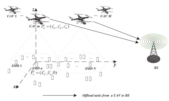
Figure 1.
Overall architecture of the system.

Table 1.
Definition of main symbols.
To strengthen the communication capability between UAVs and SMDs on the ground, current UAVs will install a directional antenna. Since the direction of a UAV directional antenna has a certain angle with the vertical direction, the range of services provided by the UAV is related to its height. As shown in Figure 2, we assume that the angle between the directional antenna of UAV j and the vertical direction is , that is, the antenna angle of UAV j is . Also, the service range of each UAV is a circle. When the antenna angle of a UAV is fixed, the service range of UAV expands as the UAV height increases; otherwise, the service range of the UAV shrinks as the UAV height decreases. Specifically, under the premise of knowing the flying height of UAV j at time slot t, we can obtain the maximum service range of UAV j at time slot t by Formula (1), and the unit of service range is square meters.
where is the PI. At the same time, the speed of information transmission between SMDs and UAVs also slows down as the distance increases. In short, to maximize the performance of the system and avoid the service quality affected caused by the UAV being too far from the ground, the UAV at any time slot should not exceed the maximum height preset by the system. Then, the flight height of UAV j at time slot t naturally meets the following restrictions, namely,
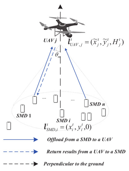
Figure 2.
The service range of unmanned aerial vehicle (UAV) j.
In this paper, after a SMD offloads the task to a UAV, the UAV will process the task immediately. When the SMD deviates from the service scope of the UAV, on the one hand, the UAV may transfer the task offloaded by the SMD to another UAV for processing to ensure the continuous service for SMD; on the other hand, the UAV may also directly transfer the task to the BS in the current area of the system. The reason why the task is directly transmitted to the base station by the UAV is that the computing power required to process the task offloaded from SMD to UAV far exceeds the maximum computing power of every UAV, the BS as a static edge server has stronger computing power than the dynamic edge server such as UAV. We describe the above two processes of transferring the task from the UAV to another UAV and from the UAV to the BS as a task migration process.
Moreover, the main content of our research is to improve the efficiency of task migration in the MEC system. Therefore, we do not consider the collaborative capabilities of UAV groups, that is, we consider that the tasks offloaded to UAVs by SMDs are inseparable. Similar to Reference [31], we do not distinguish between types of tasks. We assume that only one task is offloaded to the UAV group by SMD i at , and the task is defined as a triple, that is , where represents the total number of CPU cycles required by the computing task offloaded by SMD i. indicates the size of tasks offloaded from SMD i to the UAV group, and the unit is bit. As for , it is the maximum deadline for completing the migration of tasks offloaded by SMD i. According to Reference [32], as long as the task migration occurs in the MEC system, there will be a “migration time”, that is, the delay caused by the task migration. It can be seen that SMDs will not be able to get a more timely response to task processing results due to task migration, so reducing migration time is critical. After completing the overall description of the system, we begin to introduce the corresponding communication model of the system in the next section.
3.2. Communication Model
In this section, we introduce the communication model, which consists of three parts, namely the communication between SMDs and UAVs, the communication between UAVs and other UAVs and BS, and the communication between BS and SMDs. Obviously, the three parts of the communication are all wireless rather than wired communication, so the efficiency of task transmission is mainly affected by the three aspects of distance, noise power and network bandwidth.
For the communication between SMDs and UAVs, it mainly means that SMDs in the system offload the corresponding computation tasks to the UAVs, and UAVs return the result of the tasks computation to the corresponding SMDs. Moreover, multiple SMDs can simultaneously offload tasks to the same UAV. According to Reference [33], we can know that the wireless channels between SMDs and UAVs are determined by the location of the SMD links. Therefore, the channel gains of SMD i and UAV j in time slot t is as follows,
where represents the channel gain between a SMD and a UAV when the distance is one meter, and represents the distance between SMD i and UAV j in time slot t. For simplicity, we directly use the Euclidean distance to define , that is,
Also, regarding the transmission rate between SMDs and UAVs, according to Reference [34], the rate of wireless transmission is mainly determined by four aspects: network bandwidth, channel gain, transmission power, and noise power. We define the transmission rate of SMD i offload tasks to UAV j in time slot t, that is,
where represents the channel bandwidth between SMD i and UAV j, and represents the noise power between SMDs and UAV group. represents the transmission power of SMD i offload task to UAV j at time slot t. In particular, in real application scenarios, SMDs rely on battery power, which means that the energy of SMDs is limited. In addition, the transmission power mentioned in the previous content will directly affect the residual energy of the battery, so we set the maximum transmission power of SMD . So satisfy the following inequality,
For the communication between UAV and other UAVs and BS, it mainly means that UAVs can transfer the computation tasks that cannot be processed to other UAVs or BS, and multiple UAVs can also transfer tasks to the same UAV or BS at the same time. It should be noted that since the task migration between UAV and the task migration between UAV and BS involves the same communication principle, we only describe the communication process between UAVs and BS. Similar to the communication process in the first part, we use to represent the channel gain between UAV j and the BS. The specific formula is as follows,
where represents the channel gain between UAV and the BS when the distance is one meter. represents the distance between SMD j and BS in time slot t, and the specific definition is as follows,
In addition, the transmission rate and the constraint of the transmission power of UAV j transfer the task to the BS at time slot t are shown in Formulas (9) and (10), respectively.
where and are the channel bandwidth between UAV j and the BS and the noise power between the UAV group and the BS, respectively. is the maximum transmission power of the UAVs in the system. In addition, the transmission rate and transmission power of task migration between UAVs are defined as and , respectively. And and satisfy and , respectively.
3.3. Delay Model
In this section, we introduce the delay model of the system. Before introducing in detail, we first describe the specific process of task migration. Figure 3 shows the specific process of task migration by UAV j, where represents the computing resource allocated to SMD i by UAV j. And the meaning of is the time required for UAV j to process task offloaded by SMD i. With the rapid growth of the number of real-time applications in SMDs, the length of time the edge server spends processing tasks will seriously affect the service quality of the users. We did a survey, the survey results show that: when the threshold is greater than 1.2 s, the number of users is the highest, which users believe has seriously affected the service quality. Therefore, we assume that once UAV j processes a task for more than 1.2 s, it is considered that the computation power required by the task exceeds the maximum computation power of UAV j. Whether the time spent by UAV j in processing tasks exceeds 1.2 s corresponds to two cases. Case 1, When UAV j processes a task for more than 1.2 s, to ensure that the task can be processed smoothly and provide good service for SMD i, UAV j needs to migrate the task to another UAV or the BS, and then rely on the another UAV that still has strong computing power or the BS with stronger computation power than UAVs to handles task . Case 2, when UAV j does not spend more than 1.2 s processing task , UAV j still handle task offloaded by SMD i.
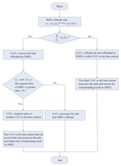
Figure 3.
Service range of UAV j.
Under case 2, to scientifically and efficiently determine the task migration timing of UAV j, we define the following two task migration triggering conditions. One of the triggering conditions is , which indicates that SMD i has left the service range of UAV j at time slot t. At this time, to continue to provide services to SMD i, UAV j needs to migrate the task that has been offloaded onto it. Another trigger condition is based on the focus on the quality of user service in this paper. Specifically, each UAV in the system will regularly send a very small data packet to the SMDs within its service range. After receiving the data packet, the SMDs will send a response to the UAV. Through the above operations, we can calculate the “response time” of SMDs. We believe that if the “response time” of SMD i is greater than 1.5 s, it indicates that the service quality of SMD i is not good, and task in UAV j needs to be migrated. In summary, as long as one of the above two conditions is met, task migration is required.
When SMD i offloads task to UAV j and the computing resources required by the task do not exceed the maximum computing power of UAV j, UAV j allocates the corresponding computing resources to SMD i and starts processing task . In the previous content, we have defined to represent the computing resources allocated to SMD i by UAV j , so the time required by UAV j to process task is defined as
When task migration conditions in Figure 3 are met, UAV j will migrate the task to another UAV or the BS. Therefore, the time for UAV j to migrate task is defined as follows,
Since the transmission speed changes with time, we use the average transmission speed for calculation. Also, also needs to meet the following restrictions, that is,
In other words, in the process of task migration, we must ensure that the migration time of task is transferred to another UAV or the BS cannot exceed , so as to guarantee the service quality of the users.
From the previous content, we know that UAV may receive multiple task requests from multiple SMDs at the same time. Here, we assume that the process of offloading tasks from SMDs is continuous. Therefore, we use to denote the length of the task queue of UAV j at time slot t, and the specific definition of is as follows,
where represents the program that UAV j must execute to maintain the normal operation of UAV j, such as the operating system. As for , it is the total number of UAV j processing tasks in time slot t, in bits. And satisfies the following equation, that is,
where c is the CPU cycles required by a UAV to handle any type of computing task.
Although UAVs have much more computing power than SMDs, their computing and storage capabilities are also limited. Therefore, and satisfy inequality (16) and inequality (17), respectively.
where is the maximum computing power of UAV.
where is the maximum storage space corresponding to the task queue of UAV.
In addition to some delay overhead, the system also has energy consumption overhead. Therefore, we introduce the energy consumption model of the system in detail below.
3.4. Energy Consumption Model
In this section, we introduce the energy consumption model of the system. We focus on the energy consumption of three parts, namely the flight energy consumption of UAVs, the computing energy consumption of UAVs, and task migration energy consumption of UAVs.
For flight energy consumption of UAVs, according to Reference [35], it can be known that the flight energy consumption of a UAV is mainly determined by the flight speed, acceleration, and altitude of the UAV. The flight speed (m/s) and acceleration (m/s) of UAV j at time slot t are defined as follows, respectively.
Therefore, we can get the flight energy consumption of UAV j during time slot t, that is,
where , and satisfy Equations (21)–(23), respectively.
where (kg/m) represents the air density in the flying area of the UAVs, and is the mass of UAV j.
where stands for PI, and w (m/s) is wind speed. As for , it is the number of revolutions per second of the propeller of UAV j.
where g is the acceleration of gravity.
Besides, during the flight of the UAVs, we also restrict the speed, acceleration, and trajectory of the UAVs, and these restrictions corresponding to inequality (24), inequality (25), and inequality group (26), respectively.
Among them, and are respectively the maximum speed and maximum acceleration of the UAV in flight, while and respectively represent the initial position and final position of the UAV. is a non-negative small value.
For the computed energy consumption of the UAVs, it mainly refers to the energy consumed by the UAVs to process the task of SMDs offload. The computed energy consumption of UAV j in time slot t is expressed as follows, that is
where k is the effective switching capacitance of the CPU in the UAV group and is determined by the hardware architecture of the CPU [36].
As for the task migration energy consumption generated by UAV, as the name implies, which is the transmission energy consumption caused by UAV during task migration. The migration energy consumption is mainly determined by the transmission power of UAV. We use to denote the energy consumption of UAV j migrate tasks to other UAVs or the BS in time slot t, and the specific definition is as follows,
In summary, the total energy consumption of UAV j in time slot t is expressed as follows, that is,
where , , and are weighting factors, which coordinate the proportion of the three energy consumptions of UAVs’ flight energy consumption, UAVs’ computing energy consumption and UAVs’ migration energy consumption.
3.5. Problem Formulation
In the previous content of the paper, we introduced the UAV-enabled MEC system and established mathematical models from four aspects, that is, architecture, communication, delay, and energy consumption. To sum up, we have three main optimization goals, and as shown below.
- Reduce the energy consumption of UAVs. Since the power of UAVs is limited, it is particularly important to reduce the energy consumption of UAVs. In the previous mathematical model, we have learned that the energy consumption of UAVs is mainly related to the three aspects of flight energy consumption, computing energy consumption, and migration energy consumption. Since the flying range of UAVs is fixed, we mainly extend the stagnation time of UAVs by reducing the computational energy consumption and migration energy consumption, to avoid some UAVs from leaving the UAV group early due to excessive energy consumption.
- Achieve the load balancing of the UAV group. When the MEC system needs to migrate SMD offload tasks, in addition to the migration energy consumption, we also need to pay close attention to the load status of each UAV in the UAV group. If load of a certain UAV is too high, we will not use it as an “endpoint edge server” to provide services to SMDs, so the MEC system will choose a UAV with a lower load to provide services to SMDs. In the end, we can make full use of the computing resources of the UAV group and achieve load balancing for the entire UAV group.
- Improve the service quality of the users. In addition to the above two points, user service quality cannot be ignored. In the process of dynamically migrating tasks offloaded by SMDs, it is inevitable that “service interruption” will occur. We believe that the shorter the service interruption time, the higher the service quality of the users. In this model, we will set a threshold. If the time required for task migration is higher than the threshold, we will not adopt this migration strategy and choose another migration strategy to complete the dynamic migration of tasks for SMDs until the migration time is less than the threshold, so as to ensure service quality of the users.
In summary, we define the following objective function, and also include the above Equations (2), (6), (10), (13), (16), (17) and (24)–(26).
where represents the migration strategy. represents a minimum error value. The purpose of setting the minimum error value is to improve the robustness in the MEC system. As for , it is a threshold used to limit the task migration time. The inequality and are to ensure that the load balancing of the UAV group and the service quality of the users, respectively.
Obviously, there are many variables in problem , and these variables will change with time, making it difficult to find the optimal solution, so we use the Markov decision model to find the optimal task migration strategy.
4. Dynamic Task Migration Strategy
4.1. Markov Decision Processes with Unknown Rewards (MDPUR)
In this section, we will introduce the algorithm of the paper. In the UAV-enabled MEC scenario, the information interaction between the MDs and the UAVs is affected by the environment, such as the wind speed and air density that we mentioned earlier. Besides, the service quality of the users is also the focus of our attention. In summary, how to get the optimal migration strategy under the circumstances of not only paying attention to environmental factors but also considering service quality has become a difficult point.
In this paper, we use the MDPUR algorithm to solve this problem. The MDPUR algorithm is different from the traditional MDP. The MDPUR algorithm is an improvement over MDP. In particular, the MDPUR algorithm reduces the number of value iterations utilizing classification and filtering, thereby increasing the speed of the algorithm. The specific improvements of the MDPUR algorithm are as follows.
- Consider the dominance vector. In the process of solving the optimal migration strategy, we considered the dominance vector. In a given initial state, each action will change the state of the UAVs. And we will classify the result of value iteration. The advantage of this is that it can improve the accuracy of solving the optimal task migration strategy.
- Improve the traditional value iteration method. The previous value iteration solution is too complicated, which will lead to high complexity of the algorithm, so we have improved on the traditional value iteration method. After each value iteration is completed, we will calculate the probability of each vector value function in the dominant vector set as the parent vector, and then select the two groups with the highest probability as the parent and perform the cross operation, and finally calculate the new descendant value function. If the result is better than all the previously calculated value functions, then use it to replace the optimal solution of the current iteration. Otherwise, give up the processing of the offspring. We call the above-mentioned value iteration method “parent crossover algorithm”, which can reduce the total number of MDPUR median iterations and increase the running speed of the MDPUR algorithm in the MEC system.
- Set dynamic UAV status. In the MDPUR algorithm, each UAV is equivalent to a node on the migration path. We define the state of the node as dynamically changing, which is more in line with the UAV-enabled MEC scenario and proves the feasibility of the algorithm. In the end, it is beneficial to apply the algorithm to real life.
In this paper, the MDPUR algorithm finally obtains the optimal task migration strategy after considering the distance of task migration, the residual energy state of the UAVs, and the load state of the UAVs. Not only does the algorithm not occupy too much computing resources of the UAVs, but it also has a very strong ability to find solutions. Especially in a dynamic environment, the MDPUR algorithm has very high flexibility and robustness. In the following content, we directly define a UAV as a node on the task migration path, which is more conducive to understanding. For example, node j represents UAV j.
4.2. Mathematical Model of the MDPUR Algorithm
In this section, we begin to establish the mathematical model on which MDPUR is based. Similar to traditional MDP, we define a six-tuple , where is the set of state space. is the set of actions, and is the state transition probability. As for and , they represent the reward function and the discount factor, respectively. The discount factor indicates the importance of future reward relative to current reward. The last item in the six-tuple is the initial state distribution of the nodes. Next, we conduct a specific analysis of the above.
4.2.1. State Space Set, Action Set, State Transition Probability
Because the state of each UAV changes with time, we use to denote the state of UAV j in time slot t. Based on that the system contains M UAVs, we define to represent the state space set of the UAVs. Moreover, we consider the three aspects of the UAVs’ position, the UAVs’ residual energy, and the UAVs’ load into the state space of the MEC system. Therefore, is a triple and . Among them, is the position of UAV j in time slot t. and are the residual energy state and load state of UAV j in time slot t, respectively. Next, we introduce the residual energy state and load state of the UAVs in detail.
For the residual energy state of the UAVs, since most of the energy supply of the UAVs are derived from the lithium battery carried by itself, we define to represent the residual energy of UAV j in time slot t, in joules (J). Because we have already defined the total energy consumption of UAV j in time slot t, that is , the iteration formula of is as follows
where is the residual energy state of UAV j in the first time slot (that is, the initial energy state), and is the maximum residual energy of UAV j. To understand the residual energy state of UAV j in time slot t more intuitively, we define as a percentage, which can intuitively represent the residual energy as a percentage of its maximum energy. In particular, the specific formula corresponding to is as follows.
For the load status of the UAV. We believe that the UAV task queue length can indirectly reflect the load status of the UAV, that is, the greater the UAV task queue length, the higher the UAV load. We define to represent the load state of UAV j in time slot t, the specific formula is as follows.
Similar to , is also a percentage, which can visually indicate the load status of the UAV. For example, indicates that the load of UAV j in time slot t is . At this time, UAV j needs to process a large number of tasks and the load is high.
After building the state space Set of the UAVs, we now start to build the action Set of the UAVs. In the MDPUR algorithm, when the system acts, the state of the corresponding UAV will change accordingly. There are M nodes in the paper, so we can think that the action set contains M actions. The specific formula is as follows.
where refers to the task is migrated to UAV j
As for the state transition probability, we define to represent the state transition probability that the state changes from s to after performing action a.
4.2.2. Reward Function
In general, the size of the reward function r can directly reflect whether a certain state or action is good or bad for the current state, and we can understand it as a numerical cost. In this paper, we will comprehensively consider the two information of the load state and residual energy state of the UAV. Different from the previous MDP, the value of the reward function r in this paper is obtained by the dot product calculation of two vectors, so the definition of the reward function is as follows.
where and are binary vectors. is the value of the reward function obtained by selecting action for state s. When the load of the UAV is lower, is larger. Similarly, when the residual energy of UAV is more, is larger; on the contrary, when the UAV load is higher or the residual energy is less, is smaller. In addition, and are weighting factors, which satisfy , and . Although the load state of UAV and the residual energy state of UAV are considered by the MDPUR algorithm at the same time, the priority of the two is different in different situations. The following describes the case where the load state or the residual energy state is considered first under the two conditions.
In condition 1, after the UAV group just took off, the UAVs in the UAV group have more residual energy at this time, so when the MEC system performs task migration for the task offloaded by a SMD, we first consider the load state of the UAVs, followed by the residual energy state of the UAVs. Therefore, the value of will increase and the corresponding value of will decrease. In condition 2, when , that is to say, the overall residual energy of the UAV group is low, in order to maximize the lag time of the UAVs with the lower residual energy in the UAV group, we first consider the residual energy state of the UAVs, followed by the load state of the UAVs. Therefore, the value of will decrease and the corresponding value of will increase. After introducing the reward function in the model, we will define the value function in the next section.
4.2.3. Value Function
Before introducing the value function, we first introduce a concept “long-term expected reward”, the value of the long-term reward can directly reflect the advantages and disadvantages of the strategy. In theory, we can use a long-term expected reward to evaluate the pros and cons of any strategy. In other words, the value function is the concrete expression of the long-term expected reward. The value function in this paper is different from the value function in the general MDP, the specific definition is as follows.
where represents the strategy, it is a mapping from the state set to the action set, namely . Whereas refers to taking action in state s, represents the value function of each strategy, that is, . is the next state. Formula (37) is the recursive regression form of the value function, from which we can understand that the value of a state is composed of the reward of the state and the subsequent state value in a certain proportion. And We usually call the Formula (37) the Bellman equation. Regarding , we have already introduced it earlier. It means that the conversion factor and the value range is . Especially, The role of the conversion factor is to ensure that the value function converges during the recursive process.
In this model, we also consider the initial states of the UAVs, and the formula is defined as follows.
4.3. Markov Decision Processes with Unknown Rewards (MDPUR) Algorithm
Now, we start to solve the optimal migration strategy . Among all possible MDP strategies, the expected value of is the largest, and is expressed as follows
Earlier we have carefully introduced the Markov decision process(MDP) model under the UAV-enabled MEC system. Below, we specifically explain the solution process of the joint optimization problem (30). To get the optimal strategy, we have proposed the MDPUR algorithm, which is mainly composed of two parts, namely the dominant value iteration algorithm and the parent crossover algorithm. The specific steps are as follows.
Step 1: Initialization. First, we need to collect the information of the nodes (that is, UAVs) and establish a state set and an action set . The research in the paper is to optimize the three aspects of the energy consumption of the UAV group, the load balancing of the UAV group, and the service quality of users. Therefore, this is a joint optimization problem.
Step 2: Calculate the reward function and value function. In the model, the size of the reward function r is mainly determined by the load state of the node and the residual energy state of the node, which helps the UAV group to achieve load balancing as soon as possible and improve the hang time of the UAV group. Then we can get the information of the target node through the location of the SMD, because the service range of the node may overlap, so the target node in this paper can be one or more. After we have determined the target node, we can calculate the value function.
Step 3: Dominant value iteration. Before iterating over the dominant value, we need to set a threshold and then start the first iteration of the value function. If the absolute value of the mathematical expected difference between the value function of the n-th iteration and the value function of the (n + 1)-th iteration is less than (that is, is satisfied), then stop the iteration and execute step 5 directly; Otherwise, continue execute step 3. After each iteration, we will classify the value function and determine the dominant value function in this iteration, and then execute step 4.
Step 4: Perform the parent crossover (PC) algorithm. We use the parent crossover algorithm to process the dominant value function and update the calculation result to the new dominant value function set, and then continue to Step 3.
Step 5: Determine the optimal migration strategy . When the iteration is completely stopped, we will sort the value function of the last iteration according to the size of absolute value and choose 5 optimal strategies, and then we will calculate the total energy consumption of the corresponding UAV group. The strategy with the lowest total energy consumption is the optimal strategy . If the migration time corresponding to the strategy does not satisfy the Formula (32), return to Step 3 to recalculate.
Next, we will separately introduce how to use the advantage-based value iteration algorithm and the parent crossover algorithm to solve the optimal migration strategy and analyze the performance of the MDPUR algorithm.
4.3.1. Advantage-Based Value Iteration (ABVI) Algorithm
In this section, we propose a new algorithm. We call this algorithm an advantage-based value iteration (ABVI) algorithm. Next, we introduce how to use the ABVI algorithm to get the optimal strategy and analyze the performance of the ABVI algorithm.
First, we define as the threshold for value iteration. When is satisfied, the value iteration is stopped. Before performing the ABVI algorithm, we need to know how to calculate the corresponding strategy through the value function. Here, we define an intermediate variable that is often used in the solution process, namely the action value function , which is described as follows.
where refers to the choice of action in state s, and other states adopt the expected reward of strategy . When the strategy does not display records and only has the value function , the action value function is recorded as Q. And the strategy can be calculated by the following formula.
At the same time, we calculate the difference between the action value function and the value function , the specific formula is as follows.
In addition, because the paper also considers the distribution of the initial state of the node, the difference between and corresponding to the mathematical expectation is as follows.
Moreover, in Formula (42) and in Formula (43) can also be called advantages, and these two values will be applied in the later iteration of the advantage value. The so-called advantage-based value iteration is to transform the traditional value function into a vector value function, and then iterate the value. After each iteration, we compare and classify these vector-valued functions. Then, the advantage-based value function set continues to the next round of value iterations until it is satisfied stops iterating.
In the process of advantage-based value iteration, it is undoubtedly very difficult to compare vector-valued functions. Here, we define two methods for comparing vectors. The first vector comparison method is pareto dominance, which is a very common vector comparison method and described in Definition 1.
Definition 1.
For a given twod-dimensional vectors and , we can know
when is satisfied, vector is better than vector .
The second vector comparison method is the vector dot product. In the previous content, we defined . For a given two two-dimensional vectors, and , we have
Here, we will calculate the dot with and , respectively. Because they are two-dimensional vectors, the calculation result is a real number, and then we compare the vectors by comparing the size of the two real numbers.
Next, we begin to define the vector value function, because the reward function of this paper is mainly determined by the load state and residual energy state of the nodes, so the corresponding vector value function is two-dimensional, the specific formula is as follows.
Among them, is a two-dimensional vector, and it is calculated from vector and vector . As for the calculation method, it is a new vector formed by multiplying the corresponding elements in the vector.
After determining the vector value function, we can easily get the mathematical expectation of the vector value function considering the initial state distribution of the node, and it is expressed as follows.
In the process of vector value iteration, we also need to define to solve the set of advantage-based value function, and is expressed as follows.
Definition 2.
If is not the optimal vector value function, then there must be a state that makes true after selecting action .
Because the only difference between and is state , the vector action value function satisfies the following inequality.
Next, we take and as examples to analyze the advantages of . Therefore, Equation (50) can be obtained.
In Formula (51), is the difference between the mathematical expectation of the vector value function and the mathematical expectation of the vector value function , which is also called the advantage of the vector. Because the difference between and is the state , we can finally get the advantage of by combining Formulas (50) and (51), that is,
The above is the process of the first round of vector value function iteration. In the subsequent iterations, we assume that , , or may appear in addition to . Therefore, we define to indicate that the state selects the action in the second round of iteration. Moreover, the role of is similar to the previous . Hence, we have inequality (53) in the second round of value iteration.
Correspondingly, the advantages of the vector value function in the second round are as follows.
To speed up the iteration and try to reduce the complexity of the algorithm, we will use the parent crossover algorithm to process the set of advantage vectors after each iteration. And the parent crossover algorithm will be introduced in detail in the next section. Moreover, the ABVI algorithm also considers the initial distribution of the nodes. The pseudo code of the ABVI algorithm is described in Algorithm 1. In Algorithm 1, is the set of advantage vectors, and n is the number of iterations.
| Algorithm 1 The proposed ABVI algorithm |
Input: Output:
|
4.3.2. Parent Crossover (PC) Algorithm
In this Section, we introduce the parent crossover algorithm that is, Algorithm 2 in the paper.
The idea of the algorithm comes from the ant colony optimization (ACO) algorithm. The algorithm performs a cross operation on a better solution, thereby increasing the possibility of seeking the optimal solution. In Algorithm 1, a new set of advantage vectors will be generated after each round of iteration, and the role of Algorithm 2 is to process these advantage vectors. For Algorithm 2, more specifically, we first need to calculate the probabilities of these vectors as the parent and then select two vectors with the highest probability as the parent vector for the cross operation. Finally, we get the new vector after the cross operation. If the new vector is better than the optimal vector value function in the advantage vector set, the new vector is added to the advantage vector set; otherwise, the advantage vector set is not processed. The parent crossover algorithm is shown in Algorithm 2 in the form of pseudo code.
| Algorithm 2 The proposed PC algorithm |
Input: Output:
|
5. Experimental Results and Discussion
In this section, we use Matlab software to do simulation experiments and evaluate the performance of the ABVI algorithm based on the experimental results. Finally, we proved the efficiency and feasibility of the ABVI algorithm through experiments. Next, we will describe the four aspects of the total energy consumption of the UAV group, the task migration time, the load state of the UAV group, and the flight time of the UAV group.
5.1. Setting of Experimental Parameters
In the simulation experiment of this paper, we set a flying area of a UAV group, the area is a rectangle of 1000 m m. The UAV group provides services for SMD in this area. The horizontal movement range of each UAV is 550 square meters. Each UAV has a fixed flight trajectory during flight and the respective flight trajectories do not overlap. In the paper, the UAV-enabled MEC system includes both a dynamic edge server (that is, the UAV group) and a static edge server (that is, a BS). The maximum service range of each UAV in the UAV group is a circular area with a radius of 170 m, and the service range of UAV will also change with the change of UAV height. In addition, other relevant experimental parameters in this paper are defined in Table 2.
Table 2.
Definition of the main experimental parameters.
In the ABVI algorithm of the paper, we also set and . In the following experiment, in order to be more convincing, we also introduced three algorithms of the traditional value iteration (TVI), ant colony optimization(ACO), and distance-based MDP (MDP-SD) to compare with the proposed ABVI algorithm. For ACO algorithm, when ants are looking for food sources, they can release a hormone called pheromone on the path they travel, so that other ants within a certain range can detect it. When there are more and more ants passing through some paths, there will be more and more pheromone, and the probability of ants choosing this path will be higher. As a result, the pheromone on this path will increase again, and the ants will follow this path. The probability of road increases again.
5.2. Analysis of the Total Energy Consumption of the UAV Group
Now, we analyze the total energy consumption of the UAV group. Because the energy of UAVs is limited, it is very necessary to reduce the energy consumption of UAVs. In the previous content, we have introduced the energy consumption model of UAVs, and we found that reducing the cost of task migration is very effective for reducing the total energy consumption of the UAV group. Therefore, we can know that the quality of the migration strategy will directly affect the total energy consumption of the UAV group. The specific experimental results are shown in Figure 4.
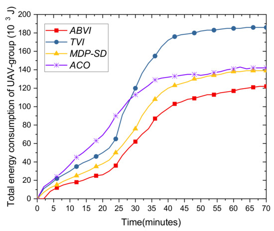
Figure 4.
The total energy consumption of the UAV group versus time.
In this experiment, we assume that there are 200 SMDs in the experiment to offload tasks to the UAV group, and the actual number of tasks that need to be migrated after reaching the UAV group conforms to the Poisson distribution. The ordinate of Figure 4 represents the total energy consumption of the UAV group, and the unit is kilojoule. From Figure 4, we can find that the total energy consumption of the UAV group increases with time. Between 0 and 19 min, there are relatively few tasks that need to be migrated for tasks offloaded by SMDs, so the total energy consumption of the UAV group is growing at a slower rate. Between 20 and 35 min, the total energy consumption of the UAV group has grown very fast. Between 36 and 79 min, the growth rate of the total energy consumption of the UAV group began to slow down, because the number of tasks that require task migration begins to decrease. From the experiment, we can find that the curves corresponding to the three algorithms are not smooth. That is because during the flight of the UAVs, it will be affected by environmental factors such as air density and wind speed, so the total energy consumption of the UAV group will be some irregular changes. In addition, we can also find that the total energy consumption of the UAV group corresponding to the ABVI algorithm is the lowest, the total energy consumption of the UAV group corresponding to the MDP-SD algorithm is second lowest. However, the total energy consumption of the UAV group corresponding to the TVI algorithm is the highest. The main reason for this result is that both the ABVI algorithm and the MDP-SD take distance as an influencing factor into the model, so the migration path is generally a smaller distance, and the corresponding migration costs will also be lower. In contrast, the TVI algorithm does not consider the effect of distance on migration costs.
In summary, the proposed ABVI algorithm is effective for reducing the total energy consumption of the UAV group.
5.3. Analysis of Task Migration Time
In this section, we analyze whether the ABVI algorithm can shorten the task migration time to improve the service quality of the users through experiments. As we have mentioned earlier, in the MEC system, shortening task migration time is very important to improve the service quality of the users. The specific experimental results are shown in Figure 5, and the experimental parameters we set are the same as in Figure 4.
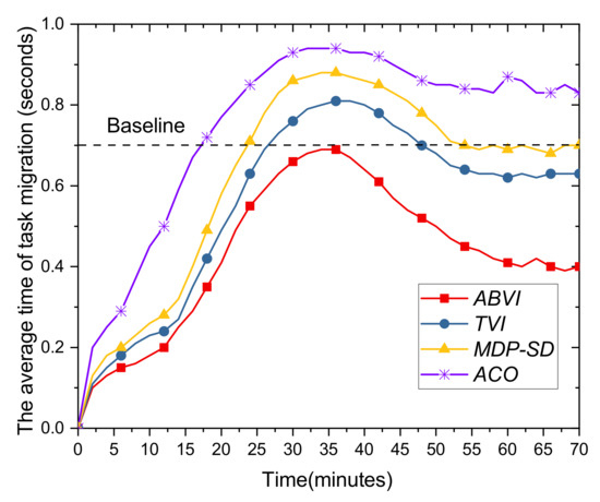
Figure 5.
The average task migration time versus time.
In Figure 5, the abscissa represents time in units of minutes, and the ordinate represents average task migration time in seconds. ACO is ant colony optimization. ABVI is the proposed in this paper, TVI and MDP-SD represent the traditional value iteration algorithm and the distance-based MDP algorithm, respectively. Here, the average task migration time represents the average of the time it takes for all SMDs currently in need of task migration to complete the task migration. This average value can very intuitively reflect the service quality of the users. In addition, we also set a standard in the experiment, which is the baseline in Figure 5. As users have higher and higher requirements for real-time services, reducing the time required for task migration as much as possible has become our research focus. Through the experiments, we found that when the service interruption time is less than 0.7 s, the user experience will not be significantly affected. Therefore, we set the baseline to 0.7 s in the experiment. Since we assume that the number of task migrations conforms to the Poisson distribution, the number of task migrations is less between 0 and 19 min, and the average task migration time rises more slowly. However, the number of task migration begins to grow rapidly between 20 min and 35 min, so the average task migration time will also increase rapidly. As time goes on, the number of task migration begins to slowly decrease between 36 min and 70 min, and the average task migration time gradually decreases and eventually stabilizes. We can also find that the curve corresponding to the ABVI algorithm is always lower than the curves of the other three algorithms. The main reason for this result is that we have fully considered the load status of the UAV group when designing the ABVI algorithm. In contrast, the other two algorithms consider less in this respect, and the complexity of the ABVI algorithm is also lower than the other two algorithms.
In summary, the ABVI algorithm is very effective for reducing task migration time and improving the service quality of the users.
5.4. Analysis of the Load Status of the UAV Group
In this section, we analyze the influence of the ABVI algorithm on the load status of the UAV group through experiments. Here, we analyze from two perspectives, one of which is to calculate the load status of each UAV in the UAV group, and the other is to calculate the difference between the highest load and the lowest load in the UAV group, that is range. The specific experimental results are shown in Figure 6, Figure 7 and Figure 8.
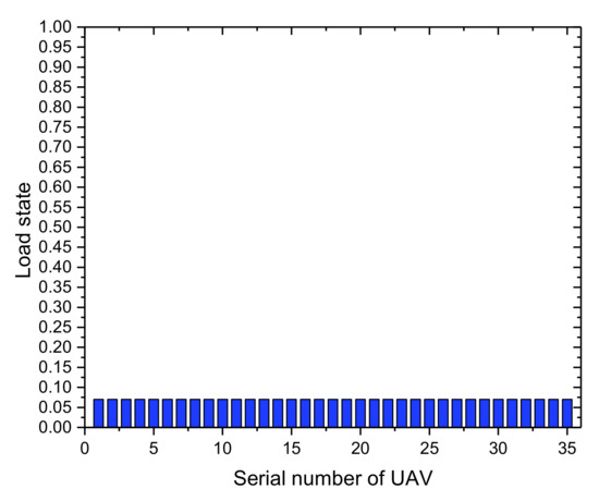
Figure 6.
The initial load state of the UAV group.
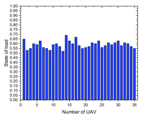
Figure 7.
The load status of the UAV group when the UAV-enabled MEC system is running for 35 min.
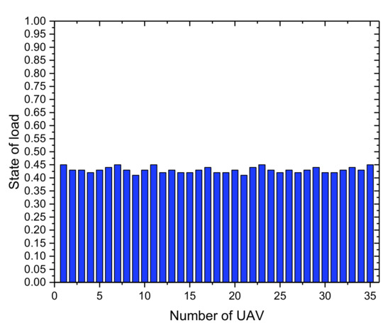
Figure 8.
The load status of the UAV group when the UAV-enabled MEC system is running for 65 min.
Figure 6, Figure 7 and Figure 8 respectively show the load state of the UAV at different times. Here, the abscissa represents the number of each UAV (i.e., ), and the ordinate represents the load status. Moreover, we use decimals to represent the load state. For example, 0.7 means that the load state of UAV is 70%, and 1 means that the UAV is at the maximum load state. When the MEC system is just running, each UAV needs to execute an operating system and other programs in the actual scenario, we set the initial load state of each UAV in the UAV group to be 0.07. Figure 6 shows the initial load state of the UAV group. Similar to the experimental parameters in the previous subsection, the UAV group receives the most tasks in 35 min, and it is also the most prone to an unbalanced load of the UAV group at this time. From Figure 7, we can find that although some of the UAVs in the UAV group have higher loads and some have lower loads, the overall trend is balanced and there is no load imbalance. At 65 min, the number of receiving tasks of the UAV group began to decrease. From Figure 8, we can find that the UAV group is still in a state of load balancing.
In summary, by counting the load status of each UAV in the UAV group at different times, we can find that the ABVI algorithm helps the UAV group achieve load balancing during the task migration process and avoiding the unbalanced loads in the UAV group.
Besides, we analyze the load status of the UAV group by calculating the difference between the highest load and the lowest load in the UAV group (i.e., range). For example, when the highest load of the UAV group is 0.9 and the lowest load is 0.2, then the difference between the two is 0.7, which is the range. The larger the range value, the more unbalanced the load state of the UAV group; otherwise, the smaller the range value, the more balanced the load of the UAV group. The specific experimental results are shown in Figure 9.
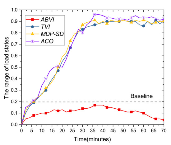
Figure 9.
The comparison of the ABVI algorithm and the other two algorithms in optimizing the load of the UAV group.
In the experiment, we set a range baseline of load states, the corresponding value of this baseline is 0.2. More specifically, when the range is less than 0.2, we think that the UAV group is in a state of load balancing. Otherwise, it is in a state of an unbalanced load. From Figure 9, we can find that the curve corresponding to the ABVI algorithm is always lower than the curve corresponding to the other two algorithms. Between 0 and 5 min, the range becomes larger. This is because the number of tasks received by the UAV groups at the beginning is relatively small, so some UAVs are vacant, and the range becomes larger. And between 6 and 70 min, the range sometimes increases slowly but also decreases. The main reason is that the ABVI algorithm considers the load status of the UAV to the reward function, so the ABVI algorithm can dynamically adjust the parameters in the algorithm and make the UAV group achieve load balancing. On the contrary, the remaining two algorithms do not take the UAV load into account, so the curve corresponding to the TVI algorithm and the MDP-SD algorithm has been increasing.
In summary, the ABVI algorithm can help the UAV group achieve load balancing, and the performance of the ABVI algorithm in optimizing the load of the UAV group is higher than the TVI algorithm and the MDP-SD algorithm.
5.5. Analysis of the Flight Time of the UAV Group
In this section, we analyze whether the ABVI algorithm can improve the flight time of the UAV group. The flight time of the UAV group is mainly determined by the residual energy of each UAV in the UAV group. In real life, when the residual energy state of a UAV is below 0.1 (that is, 10%), the UAV must exit the UAV group and land directly to the designated location. Therefore, we consider the residual energy state of the UAV as an influencing factor in the ABVI algorithm, which can avoid that some UAVs consume too much energy due to too many processing tasks and prevent UAVs withdrew from the UAV group prematurely.
In Figure 10, the ordinate represents the range of the residual energy states of the UAV group. This means that we use a range to determine whether the residual energy of the UAV group is in equilibrium. The large range means that the residual energy of some UAVs in the UAV group is too low and the residual energy of some UAVs is too high, which will cause some UAVs to consume too much energy and exit the UAV group early. However, the reduction in the number of UAVs in the UAV groups will affect the service range and service quality of the users. In this experiment, we set a baseline range of residual energy states, the corresponding value of the baseline is 0.25. When the range of residual energy states is greater than 0.25, we think that the residual energy gap of some UAVs in the UAV group is too large, which will reduce the flight time of the UAV group. On the contrary, When the range of residual energy states is less than 0.25, the residual energy gap of each UAV in the UAV group is small, and the flight time of the UAV group will also increase. From Figure 10, we can find that the curve corresponding to the ABVI algorithm has always been below the baseline.
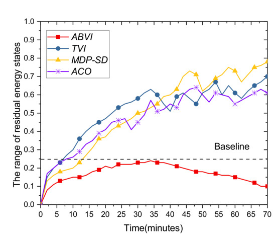
Figure 10.
The range of residual energy state versus time.
Besides, we also found that the three curves in the Figure 10 are rising from 0 to 35 min. This is because the number of task migrations needs to be following the Poisson distribution. During this time, the number of tasks that the UAV group needs to process has been increasing, so the range has grown. Between 35 min and 70 min, the curve corresponding to the TVI algorithm and the curve corresponding to the MDP-SD began to fluctuate.There are two reasons for this situation. First, because the TVI algorithm and the MDP-SD algorithm both use distance as a priority condition when choosing target migration nodes, when the number of task migrations begins to slowly decrease, some UAVs that are closer to SMDs still consume high energy, some UAVs farther away from SMDs have lower energy consumption, which causes the range of residual energy state to start to fluctuate. Second, the TVI algorithm and the MDP-SD do not fully consider the impact of the residual energy state of the UAV group on the migration strategy. As for the ABVI algorithm, it can help the residual energy of the UAV group to be in a balanced state. In Formula (38), we take the load state and the residual energy state of the UAV group into the reward function of this model, where and will be dynamically adjusted according to the average residual energy state of the UAV group, to ensure that the residual energy of the UAV group is in a balanced state and thereby improve the flight time of the UAV group. Besides, the curve corresponding to the ABVI algorithm is not smooth. The main reason is that and change dynamically during the value iteration process, so the residual energy state of each UAV group changes irregularly.
In summary, the ABVI algorithm can improve the flight time of the UAV group, and ensure the integrity of the UAV group to the greatest extent.
6. Conclusions
In this paper, we combine the dynamic edge servers (that is, the UAVs) and the static edge servers (that is, the BSs) to innovatively establish a three-layer MEC system. The purpose of this paper is to design an effective task migration strategy, which can reduce the total energy consumption of the UAV group as much as possible while ensuring the user service quality and the load balance of the UAV group. Aiming at this joint optimization problem, we established the MDPUR model and proposed the ABVI algorithm combined with the PC algorithm. Moreover, the ABVI algorithm fully considers the influence of the three factors of the load state of the UAVs, the residual energy state of the UAVs, and the migration cost on the MEC system. Finally, the simulation experiments in this paper prove that the ABVI algorithm is more efficient than the traditional TVI algorithm and the MDP-SD algorithm. Through the ABVI algorithm, we can obtain a more reasonable and effective task migration strategy, which can not only ensure the user service quality but also make the UAV group reach a load-balanced state.
Author Contributions
W.O., Z.C., J.W., G.Y. and H.Z. conceived the idea of the paper. W.O., Z.C., J.W. and G.Y. designed and performed the simulations; W.O., Z.C. and J.W. analyzed the data; Z.C. contributed reagents/materials/analysis tools; W.O. wrote the original draft; J.W. and G.Y. reviewed the paper; W.O., Z.C., J.W., G.Y. and H.Z. reviewed the revised papers. All authors have read and agreed to the published version of the manuscript.
Funding
This research was funded by The National Natural Science Foundation of China [61672540]; Hunan Provincial Natural Science Foundation of China [2018JJ3299, 2018JJ3682]; Fundamental Research Funds for the Central University of Central South University (2020zzts597).
Conflicts of Interest
The authors declare no conflict of interest.
Abbreviations
The following abbreviations are used in this manuscript:
| MEC | mobile edge computing |
| SMD | smart mobile device |
| UAV | unmanned aerial vehicle |
| BS | base station |
| MDP | Markov decision process |
| MDPUR | Markov decision process with unknown rewards |
| ABVI | advantage-based value iteration |
| PC | parent-generation crossover |
| ACO | ant colony optimization |
| TVI | traditional value iteration |
| MDP-SD | distance-based MDP |
References
- Mao, Y.; You, C.; Zhang, J.; Huang, K.; Letaief, K.B. A Survey on Mobile Edge Computing: The Communication Perspective. IEEE Commun. Surv. Tutorials. 2017, 99, 2322–2358. [Google Scholar] [CrossRef]
- Tran, T.X.; Hajisami, A.; Pandey, P.; Pompili, D. Collaborative Mobile Edge Computing in 5G Networks: New Paradigms, Scenarios, and Challenges. IEEE Commun. Mag. 2017, 55, 54–61. [Google Scholar] [CrossRef]
- Wang, S.; Urgaonkar, R.; Zafer, M.; He, T.; Chan, K.; Leung, K.K. Dynamic Service Migration in Mobile Edge Computing Based on Markov Decision Process. IEEE ACM Trans. Netw. 2019, 27, 1272–1288. [Google Scholar] [CrossRef]
- Wang, S.; Zhao, Y.; Huang, L.; Xu, J.; Hsu, C. QoS prediction for service recommendations in mobile edge computing. J. Parallel Distrib. Comput. 2019, 127, 134–144. [Google Scholar] [CrossRef]
- Lim, J.B.; Lee, D.W. A Load Balancing Algorithm for Mobile Devices in Edge Cloud Computing Environments. Electronics 2020, 9, 686. [Google Scholar] [CrossRef]
- Farhan, L.; Shukur, S.T.; Alissa, A.E.; Alrweg, M.; Raza, U.; Kharel, R. A survey on the challenges and opportunities of the Internet of Things (IoT). In Proceedings of the 2017 Eleventh International Conference on Sensing Technology (ICST), IEEE, Sydney, NSW, Australia, 4–6 December 2017. [Google Scholar]
- Zeng, Y.; Zhang, R. Energy-Efficient UAV Communication With Trajectory Optimization. IEEE Trans. Wirel. Commun. 2017, 16, 3747–3760. [Google Scholar] [CrossRef]
- Zhan, P.; Yu, K.; Swindlehurst, A.L. Wireless Relay Communications with Unmanned Aerial Vehicles: Performance and Optimization. Aerosp. Electron. Syst. IEEE Trans. 2011, 47, 2068–2085. [Google Scholar] [CrossRef]
- Huang, S.; Lv, B.; Wang, R. MDP-Based Scheduling Design for Mobile-Edge Computing Systems with Random User Arrival. In Proceedings of the 2019 IEEE Global Communications Conference (GLOBECOM), Waikoloa, HI, USA, 9–13 Dececember 2019. [Google Scholar]
- Ridhawi, I.A.; Aloqaily, M.; Kotb, Y.; Ridhawi, Y.A.; Jararweh, Y. A collaborative mobile edge computing and user solution for service composition in 5G systems. Trans. Emerg. Telecommun. Technol. 2018, 29, e3446. [Google Scholar] [CrossRef]
- Ksentini, A.; Taleb, T.; Chen, M. A Markov Decision Process-based Service Migration Procedure for Follow Me Cloud. In Proceedings of the IEEE International Conference on Communications, IEEE, Sydney, Australia, 10–14 June 2014; pp. 1350–1354. [Google Scholar]
- Wang, S.; Urgaonkar, R.; He, T.; Zafer, M.; Chan, K.S.; Leung, K.K. Mobility-Induced Service Migration in Mobile Micro-Clouds. In Proceedings of the 2014 IEEE Military Communications Conference (MILCOM), Baltimore, MD, USA, 6–8 October 2014. [Google Scholar]
- Wang, S.; Urgaonkar, R.; He, T.; Zafer, M.; Chan, K.; Leung, K.K. Dynamic Service Placement for Mobile Micro-Clouds with Predicted Future Costs. In Proceedings of the 2015 IEEE International Conference on Communications (ICC), Baltimore, MD, USA, 6–8 October 2014. [Google Scholar]
- Ceselli, A.; Premoli, M.; Secci, S. Mobile Edge Cloud Network Design Optimization. IEEE ACM Trans. Netw. 2017, 1818–1831. [Google Scholar] [CrossRef]
- Liu, J.; Mao, Y.; Zhang, J.; Letaief, K.B. Delay-Optimal Computation Task Scheduling for Mobile-Edge Computing Systems. In Proceedings of the 2016 IEEE International Symposium on Information Theory (ISIT), IEEE, Barcelona, Spain, 10–15 July 2016. [Google Scholar]
- Liu, C.F.; Bennis, M.; Poor, H.V. Latency and Reliability-Aware Task Offloading and Resource Allocation for Mobile Edge Computing. In Proceedings of the 2017 IEEE Globecom Workshops, Singapore, 4–8 December 2017. [Google Scholar]
- Liu, L.; Chang, Z.; Guo, X.; Ristaniemi, T. Multi-objective optimization for computation offloading in mobile-edge computing. In Proceedings of the 2017 IEEE Symposium on Computers and Communications (ISCC), Heraklion, Greece, 3–6 July 2017; pp. 832–837. [Google Scholar]
- Ahmed, A.; Ahmed, E. A Survey on Mobile Edge Computing. In Proceedings of the International Conference on Intelligent Systems & Control, Coimbatore, India, 7–8 January 2016. [Google Scholar]
- Chen, G. Mobile Research: Benefits, Applications, and Outlooks. In Proceedings of the Internationalization, Design & Global Development-International Conference, Idgd, Held As. DBLP, Orlando, FL, USA, 9–14 July 2011. [Google Scholar]
- Zhang, W.; Chen, J.; Zhang, Y.; Raychaudhuri, D. Towards Efficient Edge Cloud Augmentation for Virtual Reality MMOGs. In Proceedings of the The Second ACM/IEEE Symposium on Edge Computing (SEC 2017), San Jose, CA, USA, 12–14 October 2017. [Google Scholar]
- Chen, L.; Li, H. An MDP-based vertical handoff decision algorithm for heterogeneous wireless networks. In Proceedings of the Wireless Communications & Networking Conference, Doha, Qatar, 3–6 April 2016. [Google Scholar]
- Xie, S.; Chu, X.; Zheng, M.; Liu, C. A composite learning method for multi-ship collision avoidance based on reinforcement learning and inverse control. Neurocomputing 2020, 411. [Google Scholar] [CrossRef]
- Weng, P.; Zanuttini, B. Interactive Value Iteration for Markov Decision Processes with Unknown Rewards. In Proceedings of the Twenty-Third International Joint Conference on Artificial Intelligence, Beijing, China, 3–9 August 2013. [Google Scholar]
- Tetenov, A. Statistical treatment choice based on asymmetric minimax regret criteria. J. Econom. 2012, 166, 157–165. [Google Scholar] [CrossRef]
- Ruszczyński, A. Risk-averse dynamic programming for Markov decision processes. Math. Program. 2010, 125, 235–261. [Google Scholar] [CrossRef]
- Regan, K.; Boutilier, C. Robust Policy Computation in Reward-Uncertain MDPs Using Nondominated Policies. In Proceedings of the Twenty-fourth Aaai Conference on Artificial Intelligence, DBLP, Atlanta, GA, USA, 11–15 July 2011. [Google Scholar]
- Kong, L.; Ye, L.; Wu, F.; Tao, M.; Chen, G.; Vasilakos, A.V. Autonomous Relay for Millimeter-Wave Wireless Communications. IEEE J. Sel. Areas Commun. 2017, 35, 2127–2136. [Google Scholar] [CrossRef]
- Sharma, V.; You, I.; Kumar, R. Energy Efficient Data Dissemination in Multi-UAV Coordinated Wireless Sensor Networks. Mob. Inf. Syst. 2016, 2016, 8475820. [Google Scholar] [CrossRef]
- Gu, J.; Su, T.; Wang, Q.; Du, X.; Guizani, M. Multiple Moving Targets Surveillance Based on a Cooperative Network for Multi-UAV. IEEE Commun. Mag. 2018, 56, 82–89. [Google Scholar] [CrossRef]
- Guo, S.; Jiang, Q.; Dong, Y.; Wang, Q. TaskAlloc: Online Tasks Allocation for Offloading in Energy Harvesting Mobile Edge Computing. In Proceedings of the 2019 IEEE Intl Conf on Parallel & Distributed Processing with Applications, Big Data & Cloud Computing, Sustainable Computing & Communications, Social Computing & Networking (ISPA/BDCloud/SocialCom/SustainCom), Xiamen, China, 16–18 December 2019. [Google Scholar]
- Chen, X.; Jiao, L.; Li, W.; Fu, X. Efficient Multi-User Computation Offloading for Mobile-Edge Cloud Computing. IEEE ACM Trans. Netw. 2016, 2, 2795–2808. [Google Scholar] [CrossRef]
- Liu, T.; Zhu, Y.; Yang, Y.; Ye, F. Online task dispatching and pricing for quality-of-service-aware sensing data collection for mobile edge clouds. CCF Trans. Netw. 2019, 2, 28–42. [Google Scholar] [CrossRef]
- Jeong, S.; Simeone, O.; Kang, J. Mobile Edge Computing via a UAV-Mounted Cloudlet: Optimization of Bit Allocation and Path Planning. IEEE Trans. Veh. Technol. 2018, 3, 2049–2063. [Google Scholar] [CrossRef]
- Diao, X.; Zheng, J.; Wu, Y.; Cai, Y. Joint Trajectory Design, Task Data, and Computing Resource Allocations for NOMA-Based and UAV-Assisted Mobile Edge Computing. IEEE Access 2019. [Google Scholar] [CrossRef]
- Wang, L.; Huang, P.; Wang, K.; Zhang, G.; Zhang, L.; Aslam, N.; Yang, K. RL-Based User Association and Resource Allocation for Multi-UAV enabled MEC. In Proceedings of the 2019 15th International Wireless Communications and Mobile Computing Conference (IWCMC), IEEE, Tangier, Morocco, 24–28 June 2019. [Google Scholar]
- Durga, S.; Mohan, S.; Peter, J.D.; Surya, S. Context-aware adaptive resource provisioning for mobile clients in intra-cloud environment. Clust. Comput. 2019, 22, 9915–9928. [Google Scholar] [CrossRef]
Publisher’s Note: MDPI stays neutral with regard to jurisdictional claims in published maps and institutional affiliations. |
© 2021 by the authors. Licensee MDPI, Basel, Switzerland. This article is an open access article distributed under the terms and conditions of the Creative Commons Attribution (CC BY) license (http://creativecommons.org/licenses/by/4.0/).