Abstract
In this paper, we present a novel incremental learning technique to solve the catastrophic forgetting problem observed in the CNN architectures. We used a progressive deep neural network to incrementally learn new classes while keeping the performance of the network unchanged on old classes. The incremental training requires us to train the network only for new classes and fine-tune the final fully connected layer, without needing to train the entire network again, which significantly reduces the training time. We evaluate the proposed architecture extensively on image classification task using Fashion MNIST, CIFAR-100 and ImageNet-1000 datasets. Experimental results show that the proposed network architecture not only alleviates catastrophic forgetting but can also leverages prior knowledge via lateral connections to previously learned classes and their features. In addition, the proposed scheme is easily scalable and does not require structural changes on the network trained on the old task, which are highly required properties in embedded systems.
1. Introduction
“Tell me and I forget, teach me and I may remember, involve me and I learn.” (Benjamin Franklin). Natural learning systems are inherently incremental [1] where the learning of new knowledge is continued forever, ideally. For example, a finger print recognition system should be able to accept finger prints of a new person without forgetting the finger prints of already registered persons. The forgetting process is also a natural process, where a living being forgets past events unless reminded periodically. Despite the staggering recognition performance of convolutional neural networks (CNN), one area where the CNNs struggle is the catastrophic forgetting problem [2]. The degradation in the performance of a CNN network on old classes (or tasks) when a pre-trained CNN is further trained on new classes, is referred to as a catastrophic learning problem. Some researchers have also termed this problem as a domain expansion problem [3]. This happens since the weights in the network that are important for old classes are updated to accommodate the new classes.
If all the data from old classes are available, this catastrophic forgetting problem can be relieved by training the network from scratch using data from all the old and new classes. However, this raises two new problems. First, training a network from scratch (also called joint training [4]) with more data means more cumbersome training as more classes are learned during training and consequently more training time overhead. Moreover, training from scratch becomes impossible if the training data for old classes are no longer available. Second, the addition of new classes creates a data imbalance problem that directly affects the overall performance of the network.
Knowledge transfer [5,6] and zero-shot learning methods [7,8] are sometimes used to eliminate the problem of unavailability of the old training data, but the capabilities of these methods are upper bounded for their performance on old tasks. On the other hand, methods in [9,10] propose generative adversarial network (GAN) to generate old training data using generative networks [11], but the reliability of these methods heavily rely upon the generative capabilities of the GANs. So far, network distillation has been used by many researchers [1,4,12,13,14] with partial success in dealing with the missing data problem. Network distillation also eliminates the need to train the network again, and minimizes the performance degradation on old classes to a great extent. Network distillation is the process of saving the network responses on old classes, and making sure that the network is at least able to generate the same responses on a smaller set of old classes, called exemplars, during the incremental training step (after adding new classes). This, however, bounds the performance of the distilled network [15].
Nevertheless, the previous studies on incremental learning do not achieve the state-of-the-art accuracies on benchmark datasets such as CIFAR-100 [16] and ImageNet-1000 [17]. We propose a progressive incremental learning (PIL) method that uses progressive neural network architecture to incrementally learn new classes. The proposed PIL method does not require the access to old training data when training incrementally on new classes. The proposed approach (i) is able to effectively exploit transfer knowledge for compatible old and new classes and efficiently discriminate between them, (ii) is robust to the catastrophic forgetting problem, and (iii) outperforms state-of-the-art methods as well as the classical baseline incremental learning approach (joint training) on image classification task. Overall, the proposed approach corroborates the constructive, rather than destructive, nature of the progressive architecture among the related solutions for incremental learning.
2. Related Work
Li et al. [4] classified the related work on incremental learning (IL) on the basis of the underlying framework, i.e., feature extraction (the network trained on old classes is only used as feature extractor) [5], fine-tuning (the network is only fine-tuned using data from new classes) [18], and joint training (the network is trained from scratch using all the old and new classes) [19]; however, many modern incremental learning methods use a combination of these techniques. These incremental learning techniques are capable of learning new information; however, they do not satisfy all of the incremental learning criteria. For instance, they require full or partial access to old data, forget the previously trained weights or show low accuracies on new classes.
Muhlbaier et al. [20] proposed an ensemble-based approach and trained a neural network (NN) pattern classifier that can handle an increasing number of classes; however, the proposed algorithm requires training data for all the classes (old and new) at incremental learning steps. Using a small subset of all the data, Kuzborskij et al. [21] showed that the accuracy reduction in training a linear multi-class classifier due to the addition of new classes can be minimized.
Some studies partially overlap the concerns related with the IL such as unavailability of old data. For instance, zero-shot learning (ZSL) [7] or a learning task that involves recognizing categories for which there are no training examples, somehow, proposes the solution for the unavailability of old training data. Never ending image learning (NEIL) [22] can retrieve images of new classes from a few different internet platforms and establishes a relationship between them and the old classes, without prior access to the training data of those new classes. Similarly, Ref. [23] learns a model for visual variances of different classes of concepts; however, these studies only concern about maintaining the overall performance of the network [7], creating a relationship between old and unseen classes [22] and developing a visual correspondence between objects and vocabulary of visual variances [23], rather than training the network incrementally for the new classes.
The IL problem is also sometimes seen as a transfer learning problem, where the knowledge acquired on old classes (or old tasks) is applied to predict the new classes (or solve new tasks). Hence, these techniques do not rely heavily on the availability of old training data. Donahue [5] investigated semi-supervised multi-task learning of deep convolutional representations, where representations are learned on a set of related problems but applied to new tasks that have too few training examples to learn a full deep representation. Jung et al. [6] presented a method that tries to maintain the performance on old tasks by freezing the final layer and discouraging the change of shared weights in feature extraction layers. With this method, Jung et al. [6] showed that the network exhibits good transfer learning capabilities and also becomes less forgetful.
Some researchers [9,10] tried to solve the problem of the unavailability of old training data by generating them using GANs [11]; however, implementing a sophisticated GAN for complex tasks (such as unconstrained object detection) is a challenging problem. That is why the results in [10] showed that the performance drops sharply on a relatively difficult dataset [24] as compared with a simple digit classification task [25]. Moreover, these generative techniques not only add the overhead of training a separate GAN network but also require the generation of training data for incremental learning.
In contrast, knowledge distillation has been used by many researchers [1,4,12,13,14], out of which [4,14] do not require old training data at all. The good thing about these methods is that they require minimal or no network expansions, as such, they are ideal for conditions where hardware resources are limited; however, for accuracy critical situations, such as security applications, hardware resources can be traded off with consistent performance on old classes. Moreover, the knowledge-distillation-based methods, although they use no or only new examples for training, require the entire network to be trained every time a new class is to be learned.
Given the limitations of previous IL methods, we aim at developing a simple yet effective strategy on image classification tasks with CNN classifiers. We trained a progressive deep neural network incrementally, such that the performance of the network is unaffected by the addition of new classes, while the system resources are traded off. For each incremental set of new classes, an additional classifier (AC) is learned by taking the input features from the intermediate layers of the networks learned on old tasks or old networks (ONs). In this way, part of the existing network is re-used to predict the new classes with much less performance degradation as compared with its fine-tuning counterpart. Moreover, because only the portion of the network that learns the new classes is updated during the training stage, the training is much faster as compared with joint training [4]. The training also converges fast as the AC networks borrow their input from already trained convolutional layers of ONs, rather than raw image data. This mimics the knowledge transfer from previous tasks to improve convergence speed [26]. The proposed method does not require the training data of old classes at the incremental learning stages (of AC networks). Furthermore, the training also converges fast because, at each incremental learning step, the network is only optimizing the weights for a subset of classes, rather than accommodating all the old and new classes. While the increased resource utilization due to the growth of the network can be optimized by utilizing network pruning [27] and compression techniques [15].
Progressive learning is not a new domain, and several studies have already utilized progressive learning on a variety of tasks, such as reinforcement learning [28]. Progressive learning has also been previously used for optimizing network performance, where the goal is to find an optimal neural architecture design for a given image classification task [29,30]. Zhang et al. [31] used progressive learning to adapt the inference process and complexity of the neural network for images with different visual recognition complexity. His proposed scheme consisted of a set of network units to be activated in a sequential manner, with progressively increased complexity and visual recognition power.
Ye et al. [8] used progressive ensemble networks for zero-shot learning (ZSL), where the aim of ZSL is to transfer knowledge from labeled classes into unlabeled classes, to reduce human labeling efforts. The ZSL deployed a progressive training framework, to gradually label the most confident images in each unlabeled class with predicted pseudo-labels and update the ensemble network with the training data augmented by the pseudo-labels. Some researchers have also used progressive learning for improving the performance of the baseline CNNs for varieties of visual recognition tasks [32,33].
The goal of our study is to derive benefits from the progressive neural networks to incrementally learn image classifier by avoiding catastrophic forgetting phenomena. Our work is different from the fine-tuning work in [3] where the shared parameters are fine-tuned along with the parameters for the new task. In contrast, we shared convolutional layers, but the shared layers are not fine-tuned during the training process. The shared layers only act as feature extractors. Moreover, as compared with the network expansion techniques presented in [14,28,31,34,35,36,37], our proposed method consists of many architectural differences that are not only aimed at reutilizing the convolutional features learned on older tasks, but also enabling the network learned on new tasks to differentiate between old and new tasks, without additional learning (explained with details in Section 3). Below, we summarize the main contributions of this paper:
- For the first time, we experimented with a progressive neural network for incrementally learning convolutional network-based image classifiers and presented meaningful results.
- We show that the progressively learned network borrows useful information from the previously learned network to discriminate between the old and new classes, even without access to the old data, and outperforms some of the learning-without-forgetting techniques.
- By extensively experimenting with two different ResNet architectures, we provide an analysis on the trade-offs of the performance, speed and GPU resource utilization, for the progressive neural network architectures.
The rest of the paper is organized as follows. We explain the details of the proposed method in Section 3. In Section 4, we present the experimental settings and report the performances on the Fashion MNIST [38], CIFAR-100 and ImageNet-1000 datasets. We also show that the proposed scheme is able to perform better as compared to other incremental learning methods when (i) the old data are unavailable, and (ii) only exemplars are available. Finally, we conclude our work in Section 5 with a discussion about the limitations of the proposed scheme and future directions.
3. Proposed Method
The assumption is that the proposed approach keeps a frozen pool of pre-trained models throughout the training, and learns lateral connections from these along with an additional classifier (AC) network to extract useful features for the newly arrived classes. The AC network is realized by instantiating a new CNN for every group of new classes (a new row in Figure 1a), while the knowledge transfer is enabled via lateral connections to the convolutional features of the networks that are trained on old classes (represented with dashed arrows in Figure 1a).
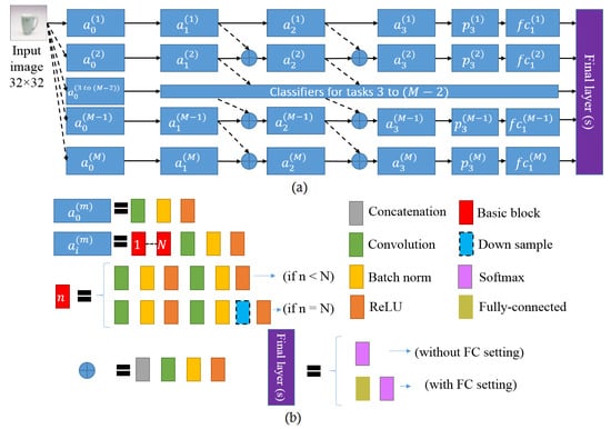
Figure 1.
Proposed architecture of the progressive network for incremental learning. (a) Each row represents an additional classifier (AC) trained on task ‘m’. (b) The implementation details of the blocks used in (a).
The proposed network can be extended and incrementally learn to adapt to any number of new classes. We demonstrate the overall method with the help of CIFAR-100 dataset, that contains 100 classes. We denote the training dataset by , where M denotes the incremental set of classes used to train each incremental step, J is the number of training samples in each incremental stage, x and y represents images and their corresponding class labels and j is the sample index inside the set of classes. The test set can be represented in a similar way. Furthermore, we denote the depth of the network with L layers containing convolutional activation blocks , where , , F, S and d represent the convolutional filter width, height, size, stride and depth (channels), respectively, at layer . We call it a convolutional activation block because it contains several convolutional, batch normalization and pooling layers, as shown in Figure 1b. Let denote the parameters to be learned for m-th set of classes, then for every new incremental set of classes, the parameters are frozen and a new additional network (as shown with rows in Figure 1) with parameters is instantiated (with random initialization), where the new layers receives activation maps from both and if and . If and , then receive activation maps from only .
The convolutional activation blocks at the same level of i are identical, which empowers the proposed method with feasibility to scale up with less complexity; however, as shown in Figure 1a, the outputs of and (for and ) are first concatenated before passing them into which causes a channel size mismatch; therefore, we added a convolution operation with the same number of filters as the number of filters in for dimension reduction. The parameters of this convolutional operation are also included in and updated during training. This not only helps to solve the channel mismatch but also adds an intelligent connection having the ability to select the best features among the current set of classes (i.e., output from ) and prior knowledge from old classes (i.e., connections from ). This concept of using lateral connections to efficiently summarize knowledge of the prior and current set of classes in the proposed method makes it unique among other approaches [14,34,35,36,37].
This method of combining previously learned features achieves a richer representation of prior knowledge which is integrated with every additional classifier network (AC) in the chain of the overall progressive network. The addition of the AC network can be considered as an additional capacity alongside the old networks (ONs), which provides the overall network the flexibility to reuse the old computations and learn the new ones, at the same time.
In order to realize the network with ResNet-18 and ResNet-101 architectures, each convolutional activation block (where ) is comprised of N ResNet basic blocks followed by batch normalization, pooling (downsampling) and ReLU operations, where and network depth = 20 and 110 for ResNet-18 and ResNet-101, respectively. As shown in Figure 1b, the downsample layer only appears in the last (n-th) basic block of each convolutional activation block (where ). Hence, the network only downsamples the input image by four times. Further implementation details about the network feature map sizes are given in Section 4.2.
The denotes average pooling layer and represents the fully connected (FC) layers for each AC network trained on a set of m classes. The ‘Final layer’ in Figure 1a comprises a softmax layer which takes the concatenated FC features from , if the old training data are not available. If the old data or exemplars from the old data are available, then the ‘Final layer’ consists of an additional FC layer (which takes the FC features from ) followed by a softmax layer. The additional FC layer is fine-tuned with the old data or exemplars from the old data. Details of experimental settings are presented in the next section.
At the training time, an AC network is added and trained with a new set of ‘’ classes by minimizing cross entropy loss on the new set of classes only. The networks trained on the old set of ‘m’ classes are only used as feature extractors, and hence successfully avoids catastrophic forgetting. Moreover, the AC networks drive their input from convolutional features of the network trained on the previous set of ‘m’ classes, rather than raw RGB features. Due to these reasons, the training processes of the proposed method is much faster than the joint training (JT) method, as shown in the results section. Unlike classical transfer learning methods [5,6], the foundation of our proposed method is not laid heavily upon the assumption that the old and new classes share some common characteristics. Rather, our method makes use of any of such characteristics flexibly.
4. Experiments and Analysis
The experimental settings were formed on the basis of our aim to predict total M sets of classes using independent classifiers by eliminating catastrophic forgetting problem and improve the learning (convergence speed and accuracy) via knowledge transfer. The brief introduction to the dataset, implementation details of the network, training strategies, experimental settings and the results are presented in the following subsections.
4.1. Dataset
We used Fashion MNIST, CIFAR-100 and ImageNet-1000 datasets for all the experiments carried out in this paper. CIFAR dataset contains 60,000 32 × 32 RGB images of 100 object classes. Each class has 500 training images and 100 test images. There were 100 classes are split into 10 incremental batches for training the network incrementally; therefore, the value of M = 10, J = 5000, in and M = 10, J = 1000, in = . ImageNet contains 1,281,167 training images and 50,000 validation images for 1000 classes, which are split into 10 incremental batches. Fashion MNIST consists of 60,000 train and 10,000 test 28 × 28 grey scale images for 10 object classes. Each class has 6000 training and 1000 test samples. For incremental training, we used an additional 1 class each time, for the total of 10 incremental batches. For the experiment setting where we train an additional FC layer with exemplar set from the old data, we select an exemplar set of 10,000 images (100 samples per class from CIFAR and FashionMNIST) using the strategy proposed in [13], but without a memory constraint. For ImageNet-1000, the exemplar set comprises 20,000 samples per class. We only use the exemplar set at the time of fine-tuning the additional FC layer (‘with FC layer’ setting).
4.2. Implementation Details
Our implementation is based on the Pytorch 1.0 library [39]. We used two network architectures throughout the experiments, i.e., ResNet-18 and ResNet-101. Due to the sequential nature of the experiments, these experiments were expected to take a longer time, so we selected these two network architectures to analyze the proposed method. ResNet-18 being quicker and smaller achieved lower limits of the speed, memory utilization and performance, while ResNet-101 achieved the upper limits of these metrics. For experimenting with ImageNet-1000 and Fashion MNIST, we only used ResNet-18.
We altered these network architectures in order to accommodate the 32 × 32 input image size of the images in CIFAR-100 dataset. As shown in Figure 1b, the features are downsampled by pooling features with size = 2 in every convolutional activation block (), and hence the depth of ResNet architecture is divided among three convolutional activation blocks for each AC network. The output size of these convolutional activation blocks at i = 1, 2, 3 is 32 × 32, 16 × 16, 8 × 8, respectively. The features after average pooling () are flattened and then passed to the FC layer (). For Fashion MNIST dataset, we simply scaled up the input images from 28 × 28 to 32 × 32, to keep the CNN architectures the same as for the CIFAR-100 dataset, while for ImageNet-1000 we resized the images to 224 × 224 and used the original ResNet architecture.
Each incremental training has 3 stages of 2000 epochs each. In order to augment the dataset and avoid overfitting, a random flip is applied to every 4th training sample. The training samples are scaled between the range of 0.16– 1, 0.08–1, 0.04–1, ratio between 0.75–1.22, 0.70–1.33 and 0.65–1.5 and then cropped to 32 × 32, for 1–2000, 2001–4000 and 4001–6000 epochs, respectively. The learning rate starts from 0.001 initially and reduces by ten times every 50 epochs until 300 epochs, after which the learning rate remains constant for up to 2000 epochs. This learning rate again becomes 0.001 and same pattern of change in the learning rate is repeated at the start of 2001st and 4001st epochs. The weight decay is set to 0.0001 and the batch size is 32, through 6000 epochs. These settings were chosen based on the initial experiments using MNIST digit dataset, and then kept the same for all experiments discussed in this paper for uniformity.
We trained the networks separately on a single GPU (NVIDIA’s RTX 2080 Ti (11GB), CUDA 10.1 and CUDNN 7.6.1) because the current implementation lacks multi-GPU processing. The machine is equipped with Intel Xeon Bronze 3104 CPU @ 1.70 GHz processor with 6 cores and 128 GB of RAM.
4.3. Results
We report the results of the proposed approach in two settings. The first one is ‘Without FC layer’, where we do not train any extra FC layer, rather we concatenate and pass the FC layer outputs () of each AC network to a final SoftMax layer. Hence, this setting is equivalent to using no old training data [4]. The purpose of this setting is to analyze the characteristic of the laterally connected AC networks, where we want to check the effectiveness of the AC networks in discriminating between old and new classes. The second is ‘with FC layer’ setting where we connect the outputs of all the to an additional FC layer and fine-tune the additional FC layer with old and the new training data. The ‘with FC layer’ setting is further divided into two modes: (i) fine-tuning the FC layer using all the training data, and (ii) by using a class-balanced set of exemplars from the train set of old and new classes. For selecting the set of exemplars, we adopted the strategy proposed in [13], but without memory constraints. In addition to comparing the proposed progressive incremental learning (PIL) method with joint training (JT), we also compared PIL with a network structure that trains an independent classifiers on each subset of incremental classes, without any lateral connections. We call the implementation without lateral connections PIL with no lateral connections (PIL-NLC). In the following subsections, we present and discuss the results of the experiments under the settings explained above.
4.3.1. Accuracy
The ‘no old data’ setting in Figure 2 means that the outputs of networks in both PIL and PIL-NLC cases are concatenated and passed to the softmax layer. Each node j of the layer corresponds to the probability score of the k-th class in the subset m. It is evident that the proposed PIL method shows superior performance over the PIL-NLC for all the three dataset. This proves the fact that the lateral connections to the prior knowledge about old classes are helpful in enabling the additional classifier (AC) networks to differentiate between old and new classes and that the PIL method positively exploits the knowledge transfer. This fact is further evident from the ‘all data’ setting in Figure 2, where all the old and new training data are used to fine-tune the additional FC layer of the PIL and PIL-NLC network. Moreover, when PIL is only trained with exemplars in contrast with JT (all data), it still outperforms JT, due to the detailed knowledge about prior information already present in the convolutional layers of the AC networks of PIL.
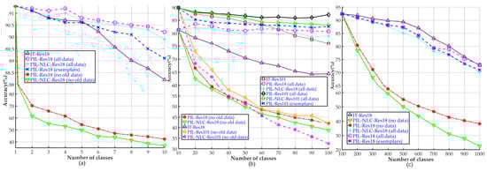
Figure 2.
Performance comparison between joint training (JT), PIL-NLC and proposed PIL using two base networks (Res18 and Res101). Performance on (a) Fashion MNIST, (b) CIFAR-100 and (c) ImageNet-1000. In all the settings, the proposed PIL scheme achieve better results than PIL-NLC scheme.
In the graph of Figure 2b, the PIL-Res101 (no old data) shows a sharp performance drop for some of the incremental steps (classes 11–20, 31–40, 51–60, 91–100), which appears unintuitive. We believe that there are two reasons for this performance drop. First, the transferred knowledge caused a convergence to poor local minima. Second, the layer decided a high local maximum probability for the old class ‘c’ due to visual similarities between a class in ‘’ and class ‘c’. This local convergence and local decision problems are solved when an additional FC layer is fine-tuned on all or exemplars of old and new data, rather than fine-tuning the entire network. As shown in Figure 2b, there is a performance gain at incremental step 91-100 after fine-tuning the additional FC layer, which shows that the PIL overcomes local and sub-optimal decisions with the help of exemplars.
Figure 2a,b also show that both PIL and PIL-NLC, when only FC layers are trained with all data, perform better than baseline method JT and also avoid catastrophic forgetting. The results on Fashion MNIST are depicted in Figure 2a, which also proves that not only PIL and PIL-NLC (all data) perform better than baseline method JT, but the PIL trained with the exemplars also performs better than the JT method with all data. Hence, the proposed method outperforms the baseline method by using only exemplars from the old data. This is due to the fact that the PIL method has better class discrimination capabilities than the baseline JT method. These networks hold more capacity to learn new weights on new classes, as well as keep the old weights (learned on old classes) frozen, while progressively learning the incremental classes. On the other hand, the JT counterpart fails to converge on optimal weights while trying to accommodate all the old and new classes. The proposed PIL method shows consistent performance on the two different datasets (RGB images in CIFAR-100 and grey images in Fashion MNIST), which proves its robustness against modality changes; however, the results on ImageNet-1000 dataset (Figure 2c), although the PIL scheme outperforms PIL-NLC scheme, it shows a little less accuracy than the JT method. We think that this is due to the fact that the ImageNet-1000 contains a large number of visually similar classes, such as 90 classes that belong to different breeds of dogs. Training the extra FC layer with exemplars helps to improve the performance, but not above the baseline JT method in case of the ImageNet-1000 dataset; another reason being the size of the images in ImageNet-1000 dataset (224 × 244), which limits the memory usage. Consequently, our experiments on the ImageNet-1000 dataset were constrained to smaller batch sizes as compared with the JT method. For JT method (which uses only one Res-18 network), we used batch size = 64, and hence JT method learns better inter-class and intra-class variances per batch. In contrast, for the PIL method (uses multiple Res-18 networks called additional networks), we could only use batch size = 2 for experiments on the ImageNet-1000 dataset; therefore, the JT method performs better than the PIL method on the ImageNet-1000 dataset.
The confusion matrices in Figure 3 also reflect the less-forgetful property of the proposed PIL method (Res101). Figure 3a shows that the PIL method does not lose performance on the first 10 classes (1–10), after the network is trained with additional 10 classes (11–20). Figure 3b,c show the performance of the PIL network after it is trained for all the 100 classes (addition of 10 classes in every incremental step); however, the network in Figure 3c contains a final FC layer, which is trained with exemplars from the old data, in contrast with the network in Figure 3b, which is not trained with old data. Despite not using old data, the PIL method achieves similar performance on old classes as compared with the performance on the new classes. Furthermore, Figure 3c shows that the performance on old and new classes improves after fine-tuning the final FC layer with exemplars from the old data. The percentage of classification errors contributed by incremental classes are tabulated in Table 1, which also proves that the PIL method does not distinguish between old and new classes. Hence, the PIL method learns new classes while it maintains the performance of the old classes.
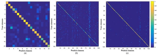
Figure 3.
Confusion matrices for the PIL method on the CIFAR-100 dataset. (a) PIL is first trained with 10 classes (1–10), and then incrementally trained for additional 10 classes (11–20) (without using old data). (b) PIL incrementally trained on all 100 classes (adding 10 classes per incremental step), without using old data and (c) using exemplars from the old classes.

Table 1.
Percentage errors incurred on old and new classes using the PIL method (FC trained using exemplars).
4.3.2. Overhead (Training Time and Memory Utilization)
The graph in Figure 4a compares the average time required to complete one training epoch by the different network implementations. All the PIL-NLC implementations show almost steady training times, due to the fact that the AC networks in PIL-NLC are independently trained on incremental set of classes. Only a slight increase in training time is recorded when the additional FC layers of PIL-NLC are fine-tuned with all the training data, because feature extraction is performed in parallel while only the additional FC layer is learned. The PIL scheme takes more time (on average) to complete one epoch as compared to PIL-NLC, due to the fact that the features from the AC networks in PIL also pass through additional convolutional operations in the lateral connections.
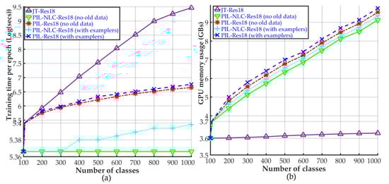
Figure 4.
(a) Training time and (b) GPU memory utilization comparison between the joint training (JT), PIL-NLC and proposed PIL methods on ImageNet-1000 dataset.
The JT shows the worst average time to complete one training epoch due to the obvious reason of the dataset size. For every incremental set of classes, the JT training routine has to pass all the training images (old + new classes) through the network to complete the epoch. On the other hand, the PIL and PIL-NLC training routines only handle the new incremental set of classes, hence much faster than the JT counterpart.
As far as the GPU memory utilization is concerned, the memory requirement trend for both PIL and PIL-NLC implementations is reflected in Figure 4b. The training time and GPU memory utilization curves for Fashion MNIST and CIFAR-100 dataset show similar trend as the training time and GPU memory utilization curves for ImageNet-1000 dataset. Moreover, the experiments on ImageNet-1000 shows the upper bounds on training time and memory utilization. Hence, we only show the curves for ImageNet-1000 dataset to avoid repetition; however, the maximum memory utilization by PIL (with ResNet-101), when the CIFAR-100 dataset is evaluated, is about 39% of the total GPU memory on NVIDIA RTX 2080 Ti, which means that 61% of the memory is still unused. The training latency of the proposed PIL can further be improved using a bigger batch size by utilizing the unused GPU resources, when the number of classes are less than 1000. As can be seen in Figure 4b, the memory utilization is still lower than the total memory of the GPU, even though the image size of ImageNet-1000 is seven times bigger than the image sizes in CIFAR-100 dataset, and the number of classes is 10 times more than the number of classes in CIFAR-100 dataset. These results show that the trade-off between the accuracy and memory utilization (only one GPU is used) is not big.
4.3.3. Comparison with the State-of-the-Art Techniques
We compare the performance (in terms of classification accuracy) of our proposed PIL method with those of the recent state-of-the-art IL techniques [1,4,12,13,40] and a baseline JT method. The implementations in [1,12,13,40] use exemplars from the old and new classes, while [4] does not use any old data. Hence, we compared these methods with the three implementations of PIL, using (i) all training data, (ii) exemplars and (iii) no old data. Figure 5a shows these comparisons, and clearly illustrates the superior performance of proposed PIL method with only using exemplars from the old and new classes. Using the same algorithm as [13] to select the exemplar set, the PIL method outperforms all the state-of-the-art schemes in terms of classification accuracy. When all the training data are available, the PIL scheme acts as an upper bound for performance comparison. In the case of the ImageNet-1000 dataset (Figure 5b), the PIL method achieves very similar performance as compared with the state-of-the-art IL technique [1] and the baseline JT method. Moreover, for the case when the number of classes are smaller than 600, the PIL method performs better than the [1] method.
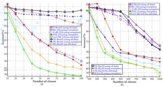
Figure 5.
Comparison of the proposed PIL method with the state-of-the-art incremental learning methods on (a) CIFAR-100 and (b) ImageNet-1000 datasets.
Figure 5a,b also show that the PIL scheme with no access to old data performs much better than the counterpart learning without forgetting scheme [4]. This confirms that the AC networks in PIL are indeed taking advantage of the features learned by the networks trained on old tasks (ONs). To ensure the uniformity in the experiments, we trained the AC networks in PIL with a fixed batch size, and up to a fixed number of epochs. We believe that more performance gains can be extracted from the proposed PIL method (under all settings) with extensive experiments by exploring different combinations of the training parameters.
5. Conclusions and Future Work
Progressive networks are immune to catastrophic forgetting by design as they naturally accumulate experiences from old tasks, making them an ideal choice for handling the catastrophic learning problem in convolutional neural networks. Hence, in this paper, we presented a novel progressive CNN architecture with lateral connections to the pre-trained networks as a solution to the catastrophic forgetting problem. With experiments, we validated our hypothesis that these lateral connections to pre-trained networks enable the overall network to differentiate (to some extent) between old and new classes without using old training data. It is shown that the proposed method outperforms state-of-the-art incremental learning techniques in terms of accuracy by using exemplar sets on CIFAR-100 dataset, and achieves similar performance on ImageNet-1000 dataset. The proposed method is scalable and shows consistent image classification performance when trained with incremental sets of new classes from the Fashion MNIST, CIFAR-100 and ImageNet-1000 datasets.
This paper also presents limitations associated with progressive neural networks. The nature of the training in progressive learning is sequential, which mainly kept us from quickly evaluating the proposed technique using different network architectures, such as ResNext and VGG with various training parameters, such as batch size, gradient and loss optimization parameters. We believe that the choice of the base network will play an important role in deciding the overall accuracy. Furthermore, the exemplar set we used is bigger than the one used by the BiC scheme, because the additional FC layer in the proposed scheme must be largely learned. The BiC scheme only used the exemplar set for bias correction in FC layers. These limitations illustrate possible future research direction. In addition, network pruning and distillation techniques can be jointly incorporated to reduce resource utilization.
Author Contributions
Conceptualization, Z.A.S. and U.P.; methodology, Z.A.S. and U.P.; software, Z.A.S.; validation, U.P.; formal analysis, Z.A.S. and U.P.; investigation, Z.A.S. and U.P.; resources, U.P.; data curation, Z.A.S.; writing—original draft preparation, Z.A.S.; writing—review and editing, U.P.; visualization, Z.A.S.; supervision, U.P.; project administration, U.P.; funding acquisition, U.P. All authors have read and agreed to the published version of the manuscript.
Funding
This work was partly supported by the Institute for Information & communications Technology Promotion (IITP) grant funded by the Korean government (MSIT) (2017-0-01772, Development of QA system for video story understanding to pass Video Turing Test) and Information & communications Technology Promotion (IITP) grant funded by the Korean government (MSIT) (2017-0-01781, Data Collection and Automatic Tuning System Development for the Video Understanding) and the ICT R&D By the Institute for Information & communications Technology Promotion (IITP) grant funded by the Korean government (MSIT) [Project Number: 2020-0-00113, Project Name: Development of data augmentation technology by using heterogeneous information and data fusions].
Conflicts of Interest
The authors declare no conflict of interest.
References
- Wu, Y.; Chen, Y.-J.; Wang, L.; Ye, Y.; Liu, Z.; Guo, Y.; Fu, Y. Large Scale Incremental Learning. In Proceedings of the IEEE/CVF Conference on Computer Vision and Pattern Recognition (CVPR), Long Beach, CA, USA, 15–20 June 2019; pp. 374–382. [Google Scholar]
- Goodfellow, I.J.; Mirza, M.; Da, X.; Courville, A.C.; Bengio, Y. An Empirical Investigation of Catastrophic Forgeting in Gradient-Based Neural Networks. arXiv 2014, arXiv:1312.6211. [Google Scholar]
- Jung, H.; Ju, J.; Jung, M.; Kim, J. Less-forgetful Learning for Domain Expansion in Deep Neural Networks. arXiv 2018, arXiv:1711.05959v1. [Google Scholar]
- Li, Z.; Hoiem, D. Learning without Forgetting. IEEE Trans. Pattern Anal. Mach. Intell. 2018, 40, 2935–2947. [Google Scholar] [CrossRef] [PubMed] [Green Version]
- Donahue, J.; Jia, Y.; Vinyals, O.; Hoffman, J.; Zhang, N.; Tzeng, E.; Darrell, T. DeCAF: A Deep Convolutional Activation Feature for Generic Visual Recognition. In Proceedings of the International Conference on Machine Learning, Beijing, China, 21–26 June 2014. [Google Scholar]
- Jung, H.; Ju, J.; Jung, M.; Kim, J. Less-forgetting Learning in Deep Neural Networks. arXiv 2016, arXiv:1607.00122. [Google Scholar]
- Lampert, C.H.; Nickisch, H.; Harmeling, S. Attribute-Based Classification for Zero-Shot Visual Object Categorization. IEEE Trans. Pattern Anal. Mach. Intell. 2014, 36, 453–465. [Google Scholar] [CrossRef] [PubMed]
- Ye, M.; Guo, Y. Progressive Ensemble Networks for Zero-Shot Recognition. In Proceedings of the IEEE/CVF Conference on Computer Vision and Pattern Recognition (CVPR), Long Beach, CA, USA, 15–20 June 2019; pp. 11720–11728. [Google Scholar]
- Shin, H.; Lee, J.K.; Kim, J.; Kim, J. Continual Learning with Deep Generative Replay. arXiv 2017, arXiv:1705.08690. [Google Scholar]
- Venkatesan, R.; Venkateswara, H.; Panchanathan, S.; Li, B. A Strategy for an Uncompromising Incremental Learner. arXiv 2017, arXiv:1705.00744. [Google Scholar]
- Goodfellow, I.J.; Pouget-Abadie, J.; Mirza, M.; Xu, B.; Warde-Farley, D.; Ozair, S.; Courville, A.C.; Bengio, Y. Generative Adversarial Nets. arXiv 2014, arXiv:1406.2661. [Google Scholar]
- Castro, F.M.; Marín-Jiménez, M.J.; Mata, N.G.; Schmid, C.; Karteek, A. End-to-End Incremental Learning. arXiv 2018, arXiv:1807.09536. [Google Scholar]
- Rebuffi, S.-A.; Kolesnikov, A.I.; Sperl, G.; Lampert, C.H. iCaRL: Incremental Classifier and Representation Learning. In Proceedings of the IEEE/CVF Conference on Computer Vision and Pattern Recognition (CVPR), Honolulu, HI, USA, 21–26 July 2017; pp. 5533–5542. [Google Scholar]
- Shmelkov, K.; Schmid, C.; Karteek, A. Incremental Learning of Object Detectors without Catastrophic Forgetting. In Proceedings of the IEEE International Conference on Computer Vision (ICCV), Venice, Italy, 22–29 October 2017; pp. 3420–3429. [Google Scholar]
- Hinton, G.; Vinyals, O.; Dean, J. Distilling the Knowledge in a Neural Network. arXiv 2015, arXiv:1503.02531. [Google Scholar]
- Krizhevsky, A. Learning Multiple Layers of Features from Tiny Images. 2009. Available online: https://www.cs.toronto.edu/~kriz/learning-features-2009-TR.pdf (accessed on 14 July 2021).
- Russakovsky, O.; Deng, J.; Su, H.; Krause, J.; Satheesh, S.; Ma, S.; Huang, Z.; Karpathy, A.; Khosla, A.; Bernstein, M.; et al. Imagenet large scale visual recognition challenge. Int. J. Comput. Vis. 2015, 115, 211–252. [Google Scholar] [CrossRef] [Green Version]
- Girshick, R.B.; Donahue, J.; Darrell, T.; Malik, J. Rich Feature Hierarchies for Accurate Object Detection and Semantic Segmentation. In Proceedings of the IEEE Conference on Computer Vision and Pattern Recognition (CVPR), Columbus, OH, USA, 23–28 June 2014; pp. 580–587. [Google Scholar]
- Zhou, Z.; Shin, J.Y.; Zhang, L.; Gurudu, S.R.; Gotway, M.B.; Liang, J. Fine-Tuning Convolutional Neural Networks for Biomedical Image Analysis: Actively and Incrementally. In Proceedings of the IEEE Conference on Computer Vision and Pattern Recognition (CVPR), Honolulu, HI, USA, 21–26 July 2017; pp. 4761–4772. [Google Scholar]
- Muhlbaier, M.; Topalis, A.; Polikar, R. Learn++.NC: Combining Ensemble of Classifiers With Dynamically Weighted Consult-and-Vote for Efficient Incremental Learning of New Classes. IEEE Trans. Neural Netw. 2009, 20, 152–168. [Google Scholar] [CrossRef]
- Kuzborskij, I.; Orabona, F.; Caputo, B. From N to N + 1: Multiclass Transfer Incremental Learning. In Proceedings of the IEEE Conference on Computer Vision and Pattern Recognition (CVPR), Portland, OR, USA, 23–28 June 2013; pp. 3358–3365. [Google Scholar]
- Chen, X.; Shrivastava, A.; Gupta, A. NEIL: Extracting Visual Knowledge from Web Data. In Proceedings of the IEEE International Conference on Computer Vision (ICCV), Sydney, Australia, 1–8 December 2013; pp. 1409–1416. [Google Scholar]
- Divvala, S.K.; Farhadi, A.; Guestrin, C. Learning Everything about Anything: Webly-Supervised Visual Concept Learning. In Proceedings of the IEEE Conference on Computer Vision and Pattern Recognition (CVPR), Columbus, OH, USA, 23–28 June 2014; pp. 3270–3277. [Google Scholar]
- Netzer, Y.; Wang, T.; Coates, A.; Bissacco, A.; Wu, B.; Ng, A.Y. Reading Digits in Natural Images with Unsupervised Feature Learning. 2011. Available online: http://ufldl.stanford.edu/housenumbers/nips2011_housenumbers.pdf (accessed on 14 July 2021).
- Yann, L.C.; Corinna, C. MNIST Handwritten Digit Database. 2010. Available online: http://yann.lecun.com/exdb/mnist/ (accessed on 14 July 2021).
- Taylor, M.E.; Stone, P. An Introduction to Intertask Transfer for Reinforcement Learning. AI Mag. 2020, 32, 15–34. [Google Scholar] [CrossRef] [Green Version]
- He, Y.; Kang, G.; Dong, X.; Fu, Y.; Yang, Y. Soft Filter Pruning for Accelerating Deep Convolutional Neural Networks. arXiv 2018, arXiv:1808.06866. [Google Scholar]
- Rusu, A.A.; Rabinowitz, N.C.; Desjardins, G.; Soyer, H.; Kirkpatrick, J.; Kavukcuoglu, K.; Pascanu, R.; Hadsell, R. Progressive Neural Networks. arXiv 2016, arXiv:1606.04671. [Google Scholar]
- Liu, C.; Zoph, B.; Neumann, M.; Shlens, J.; Hua, W.; Li, L.J.; Fei-Fei, L.; Yuille, A.; Huang, J.; Murphy, K. Progressive Neural Architecture Search. arXiv 2018, arXiv:1712.00559. [Google Scholar]
- Perez-Rua, J.M.; Baccouche, M.; Pateux, S. Efficient Progressive Neural Architecture Search. arXiv 2018, arXiv:1808.00391. [Google Scholar]
- Zhang, Z.; Ning, G.; Cen, Y.; Li, Y.; Zhao, Z.; Sun, H.; He, Z. Progressive Neural Networks for Image Classification. arXiv 2018, arXiv:1804.09803. [Google Scholar]
- Wang, J.; Sun, K.; Cheng, T.; Jiang, B.; Deng, C.; Zhao, Y.; Liu, D.; Mu, Y.; Tan, M.; Wang, X.; et al. Deep High-Resolution Representation Learning for Visual Recognition. IEEE Trans. Pattern Anal. Mach. Intell. 2020. [Google Scholar] [CrossRef] [Green Version]
- Liu, Y.-D.; Wang, Y.; Wang, S.; Liang, T.; Zhao, Q.; Tang, Z.; Ling, H. CBNet: A Novel Composite Backbone Network Architecture for Object Detection. In Proceedings of the AAAI Conference on Artificial Intelligence, New York, NY, USA, 7–12 February 2020. [Google Scholar]
- Sarwar, S.S.; Ankit, A.; Roy, K. Incremental Learning in Deep Convolutional Neural Networks Using Partial Network Sharing. IEEE Access 2020, 8, 4615–4628. [Google Scholar] [CrossRef]
- Sun, G.; Yang, C.; Liu, J.; Liu, L.; Xu, X.; Yu, H. Lifelong Metric Learning. IEEE Trans. Cybern. 2019, 49, 3168–3179. [Google Scholar] [CrossRef] [PubMed]
- Triki, A.R.; Aljundi, R.; Blaschko, M.B.; Tuytelaars, T. Encoder Based Lifelong Learning. In Proceedings of the IEEE International Conference on Computer Vision (ICCV), Venice, Italy, 22–29 October 2017; pp. 1329–1337. [Google Scholar]
- Xiao, T.; Zhang, J.; Yang, K.; Peng, Y.; Zhang, Z. Error-Driven Incremental Learning in Deep Convolutional Neural Network for Large-Scale Image Classification. In Proceedings of the 22nd ACM International Conference on Multimedia, Orlando, FL, USA, 3–7 November 2014; pp. 177–186. [Google Scholar]
- Xiao, H.; Rasul, K.; Vollgraf, R. Fashion-MNIST: A Novel Image Dataset for Benchmarking Machine Learning Algorithms. arXiv 2017, arXiv:1708.07747. [Google Scholar]
- Paszke, A.; Gross, S.; Massa, F.; Lerer, A.; Bradbury, J.; Chanan, G.; Killeen, T.; Lin, Z.; Gimelshein, N.; Antiga, L.; et al. PyTorch: An Imperative Style, High-Performance Deep Learning Library. arXiv 2019, arXiv:1912.01703. [Google Scholar]
- Hayes, T.L.; Kanan, C. Lifelong Machine Learning with Deep Streaming Linear Discriminant Analysis. In Proceedings of the IEEE/CVF Conference on Computer Vision and Pattern Recognition (CVPR) Workshops, Seattle, WA, USA, 14–19 June 2020. [Google Scholar]
Publisher’s Note: MDPI stays neutral with regard to jurisdictional claims in published maps and institutional affiliations. |
© 2021 by the authors. Licensee MDPI, Basel, Switzerland. This article is an open access article distributed under the terms and conditions of the Creative Commons Attribution (CC BY) license (https://creativecommons.org/licenses/by/4.0/).