Development of a Portable, Reliable and Low-Cost Electrical Impedance Tomography System Using an Embedded System

Abstract

Electrical impedance tomography (EIT) is a useful procedure with applications in industry and medicine, particularly in the lungs and brain area. In this paper, the development of a portable, reliable and low-cost EIT system for image reconstruction by using an embedded system (ES) is introduced herein. The novelty of this article is the hardware development of a complete low-cost EIT system, as well as three simple and efficient algorithms that can be implemented on ES. The proposed EIT system applies the adjacent voltage method, starting with an impedance acquisition stage that sends data to a Raspberry Pi 4 (RPi4) as ES. To perform the image reconstruction, a user interface was developed by using GNU Octave for RPi4 and the EIDORS library. A statistical analysis is performed to determine the best average value from the samples measured by using an analog-to-digital converter (ADC) with a capacity of 30 kSPS and 24-bit resolution. The tests for the proposed EIT system were performed using materials such as metal, glass and an orange to simulate its application in food industry. Experimental results show that the statistical median is more accurate with respect to the real voltage measurement; however, it represents a higher computational cost. Therefore, the mean is calculated and improved by discarding data values in a transitory state, achieving better accuracy than the median to determine the real voltage value, enhancing the quality of the reconstructed images. A performance comparison between a personal computer (PC) and RPi4 is presented. The proposed EIT system offers an excellent cost-benefit ratio with respect to a traditional PC, taking into account precision, accuracy, energy consumption, price, light weight, size, portability and reliability. The proposed EIT system has potential application in mechanical ventilation, food industry and structural health monitoring.

1. Introduction

Electrical impedance tomography (EIT) is a noninvasive technique that consists in measuring an impedance array through a cross-section. This technology has been applied in many clinical applications [1,2,3], such as detection for breast cancer [4,5], nerve activity in the brain [6,7,8], respiratory disorders [9,10,11], lung function detection [12,13,14], cardiovascular monitoring [15], assessing facial nerve proximity [16]; it also has several industrial applications [17,18,19,20,21,22,23] and structural health monitoring in the construction industry [24,25,26,27,28,29,30]. The food industry also uses electrical or electrochemical impedance spectroscopy (EIS) which in simple terms is a kind of EIT by using multiple frequencies and it is used in food quality assurance to detect adulterated or polluted food, the electrical parameters of food change when they are adulterated, as well when food has a pathogen like bacteria [31,32,33,34]. The impedance of human body tissue is able to provide information about the physiological and pathological properties of the tissue, both of these properties are related to the information of medical applications [1]. EIT can be achieved by using multiple electrodes placed in a cross-section; however, this is not a mandatory and other configurations of EIT can be used. Electrodes are important components of EIT system; they must have good electrical conductivity and must be anticorrosive because an electrical current is applied through them and also used for sensing voltage. There is a research work focused on the study of electrodes, because they can be improved, for example, through sandblasting [35]. The data obtained by measuring all possible impedances is used to reconstruct an image, which may provide qualitative and quantitative information. Images of live tissues and organs can be obtained by placing electrodes on the skin and injecting a small current into the body. EIT could provide a safe and cost-effective alternative to established clinical imaging methods across a wide range of applications. However, the imaging problem is severely ill-posed (inverse problem) and ill-conditioned, which means that even relatively low noise levels in measurements could lead to significant reconstruction artifacts. In other words, the solution is highly sensitive to changes in the final data [36,37] and therefore the resulting image quality is limited [38,39].

The authors in [40] developed a highly versatile ElT system using open-source software and commercial components. The system design was shared under an open-source license and uses electronic modules and a personal computer (PC) interface. Their results can be confirmed by comparing the reconstructed images with well-known literature. Field-programmable gate array (FPGA) devices have been used to develop EIT, as shown in [41,42], basically to control and execute commands for the EIT system, leveraging the advantages they offer as programmable gates. Their complexity enabled the authors to deliver high-speed and high-performance results. Other efforts are being made for EIT algorithms based on back-projection, Fourier, Gauss–Newton and variable splitting (VS) [43]. Other authors have worked on developing an approach to EIT image reconstruction based on machine-learning algorithms, proving that neural networks are useful for EIT [44]. In Reference [45], the authors propose an efficient and high-resolution EIT image reconstruction method in the framework of sparse Bayesian learning. Significant performance improvement is achieved by imposing structure-aware priors on the learning process to incorporate the prior knowledge that practical conductivity distribution maps exhibit clustered sparsity and intracluster continuity. In Reference [46], the authors propose an efficient and high-spatial-resolution algorithm for simultaneously reconstructing multiple fdEIT (Frequency-difference electrical impedance tomography) frames corresponding to inject currents with multiple frequencies. The electrical impedance tomography reconstruction problem is considered within a hierarchical Bayesian framework, where both intratask spatial clustering and intertask dependency are automatically learned and exploited in an unsupervised manner.

Other research efforts have focused on designing nine different circuits for EIT systems and comparing three different solutions using a digital signal processor (DSP) for image reconstruction, resulting in a low-cost system [47]. The use of eight silver electrodes distributed in a ring configuration to make electrical impedance measurements is reported in [48] as a methodology for locating carcinoma, together with a proposed algorithm that is used in breast models. A study employing active electrodes for lung ventilation is reported in [49], which presented an electronic system and experimental results on a human being, proving that active electrodes can be applied for human thoracic EIT. The system communicates through Ethernet to a PC or ventilator and uses an FPGA to control impedance sampling. As can be inferred, one of the many problems with working with humans is placing electrodes in a person, and in addition, electronic noise can be generated by skin, hair or sweat. With some reservations, the authors achieved good results for future medical applications of EIT.

From a hardware viewpoint, the authors in [50] developed a parallel EIT system using multiple microcontroller units (MCUs) to perform measurements and process FFTs at the same time. The system, which reaches speeds of up to 30 frames per second, was compared to a commercial one, and an error rate of only 10% was found. The authors in [51] report the development of an EIT system with an Arduino MCU and the well-known electrical impedance and Diffuse Optical Tomography Reconstruction Software (EIDORS) [52] on a PC, using Matlab to reconstruct images. The system has a resolution of 32 electrodes and each part of the system is developed on separate PCBs. They reconstruct images, but in contrast with this paper, their ADC only has a resolution of 12 Bit, their circuits and algorithms are not described in detail, and they do not perform image reconstruction on an ES. In Reference [53], the authors report an EIT system developed using an Arduino MCU, a Raspberry Pi 3 and 16 electrodes. They show that the system reconstructs images by using Python software instead of the EIDORS [52] library for Matlab. The authors in [54] present a super-resolution imaging model for EIT, with results that show better image quality using different simulated data. On that basis, in this study the EIDORS library was used to perform image reconstruction. In addition, the authors in [55] developed an EIT system that combines the reconstruction of three different images at different frequencies, with the goal of simulating a breast tumor and showing the importance of obtaining images with different frequencies to obtain better information. More recently, the authors in [56] reviewed different studies of imaging techniques, including EIT, and reported that Acute Respiratory Distress Syndrome (ARDS) problems had only been partially resolved. The literature review leads us to assert that EIT can be employed in cases of respiratory conditions [10,56,57,58,59,60,61]. For this reason, further research and development in EIT lung imaging is crucial.

Accordingly, one can take advantage of ES, which are very useful for solving real-world problems across various fields of application [62,63,64,65,66]. To our knowledge and based on the reviewed literature, only one study reports the use of an Raspberry Pi 3 Model B [53], and one other paper reports using an Arduino MCU [51] for the development of an EIT system. However, there are still open problems to be solved, such as the development of new methods and algorithms to improve EIT systems, because the imaging problem is severely ill-posed and ill-conditioned, which means that even relatively low noise levels in measurements could lead to significant reconstruction artifacts. Thus, in this paper an RPi4 may prove useful in developing a low-cost, portable and reliable EIT system, since it can be coded by using open-source software and is inexpensive, small and lightweight; furthermore, it performs well and offers multiprocessing capabilities and easy scheduling tasks, thus enabling fast technological development. The novelty of this paper is the hardware development of a complete low-cost EIT system, as well as three simple and efficient algorithms that can be implemented on ES. Details of the new electronic circuits, firmware and functions developed in this study are presented herein. The experiments show that the proposed EIT system delivers practically the same results as those obtained with a traditional PC.

The rest of this paper is organized as follows. Section 2 describes the adjacent measurement method, the physical design of the electrical impedance measurement base (test unit), the electronic design of the circuits and the firmware and functions for the proposed EIT system. Section 3 presents the experimental results, including a comparison between a PC and RPi4, calibration and results with different materials, such as steel, glass and an orange, as an example of use in the food industry. Finally, Section 4 summarizes our conclusions.

2. Development of the Proposed EIT System

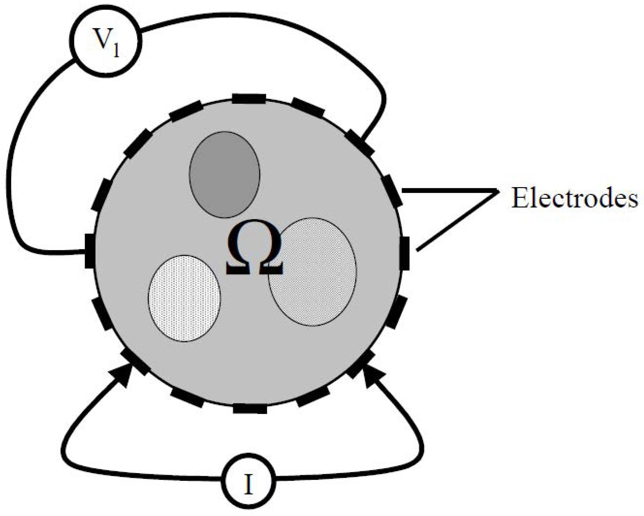
Figure 1 depicts a basic 16-electrode system. The main equation for the voltage field produced by running a current across a material corresponds to (1), where I is the current, $\sigma$ is the electric impedance of the medium, $\varphi$ is the electric potential, $\omega$ is the angular frequency, and $ϵ$ is the electric permittivity. This equation can be reduced to an equation known as the “standard governing equation for EIT” [67], given in (2),

$$\nabla ·(\sigma +I\omega ϵ)\nabla \varphi =0,$$

(1)

$$\nabla ·(\sigma \nabla \varphi )=0.$$

(2)

The problem requires the injected current I and the voltage measured $V_1$, the values of which are known and obtained from an EIT electronic system, but the impedance distribution $\sigma$ is unknown; here we cannot easily resolve $\sigma$ for  (2) because the potential distribution $\varphi$ is a function of the impedance, $\varphi =\varphi \left(\sigma \right)$. As mentioned before, here the ill-posed nature of the problem is clear from observing and understanding the diffusive behavior of electricity and the inherent measurement errors.

As a tomography technique, EIT basically reconstructs the spatial distribution of electrical conductivity within a body by measuring the voltage that appears on object boundaries due to the flowing electrical current [69]. The basic principle is to use the material’s impedance features to characterize its internal structure [70]. Some authors argue that it is an emerging method for imaging the evoked activity of a rat brain [7,71], and it can also be used in human brain injury monitoring, as reported in [72,73].

Nowadays, there are different standard configurations connecting 8, 16, 32 electrodes and also systems with 128 electrodes or more. In this paper, a 16-electrode configuration is used to test and validate the proposed EIT system. An image is generated from a test unit, which consists of a circular vessel with a conductive liquid (water with potassium chloride or sodium chloride), where the object under test is introduced, then 16 electrodes are connected to four multiplexers and to an Arduino MCU, which maps the impedance of the object under test or the body, which is measured and characterized to form an image. All features were considered in the conception of the system as a whole: the electronic design, the data acquisition (DAQ) stage, the instrumentation, the data communication and the software that receives raw data and reconstructs the image in real time.

2.1. Adjacent Measurement Method

The adjacent method for EIT consists in applying a known current to a pair of neighbor electrodes. Once the known current is applied through these electrodes, an adjacent voltage measurement is made in all the adjacent connections of the cylinder water tank (vessel). Figure 2 shows the physical appearance of the test unit (vessel) used in this paper to test and validate the proposed EIT system. It is a round plastic vessel, which was used to contain the experiment samples (salty water, metal, plastic objects, fruit etc.), then 16 stainless steel 304-caliber electrodes were placed equidistantly for the proposed EIT system. The screws were introduced into the plastic vessel using nuts and rubber washers to prevent leakage. This vessel was used for all experimental procedures for the proposed system; a shielded cable was attached to each electrode to connect the electronic system and prevent noise. The 16 electrodes of the vessel were numbered clockwise and connected to the four ADG1406 multiplexers. The MCU manages the connections to perform the required measurements. It consists of an impedance acquisition subsystem that sends the impedance measurement values through the USB port to an RPi4, which after receiving the data stream, executes software that uses the EIDORS library [52] for image reconstruction. The shape of the sample measured must be known in order to verify correct image reconstruction; this is also helpful in calibrating the image reconstruction algorithm and therefore in obtaining a better image approximation. Many mathematical models exist, depending on the shape of the test unit (vessel); for this research, a circular shape was used.

Figure 3 shows how a constant current source is applied to two neighbor electrodes, a voltage measurement is performed on the remaining pairs, and afterwards, by means of a multiplexer, the voltage source is connected to the next pair of neighbor electrodes and the adjacent voltage is measured again until all combinations are covered; in this case, for a 16-electrode base, there are 208 measurements.

2.2. Electronic Design

Figure 4 depicts the block diagram of the proposed EIT system. The hardware consists of a data acquisition (DAQ) subsystem and a user interface. The DAQ subsystem hardware was coded to employ the adjacent measurement method (Section 2.1) on the test unit. The Arduino MCU selects which pair of electrodes is connected to the AC constant current source, and the other pair that is connected to the adjacent electrodes. Then the signal is processed with the help of an instrumentation amplifier configured as a peak detector connected to an ADC that sends the voltage measurement value through an SPI (serial peripheral interface) protocol by receiving commands from the Arduino MCU, which sends the raw data through serial communication at 500,000 bps to a central processing unit (CPU), e.g., the RPi4, as is the case here.

Table 1. Proposed EIT system features.

Description	Feature
Electrical connection	110 $V_{AC}$ 60 Hz
Peak power consumption	15 W
Embedded voltage source	5 V, 12 V and −12 V
MCU	Arduino Mega 2560
Communication	Serial USB 2.0
Communication speed	500,000 bps
ADC	ADS1256 24 bit resolution at 30 kSPS
Multiplexers	Four 1 to 16 decoder ADG1406
Number of electrodes	16
Input frequencies	4–8 kHz
Frame rate	12 per minute
Connectivity	Bluetooth & USB 2.0
Networking	Ethernet & WiFi
Test unit diameter	17.5 cm

shows the system’s features, the proposed EIT system works with 110 $V_{AC}$ at 60 Hz, the peak power consumption is 15 W, it has three DC operating voltages, 5 V, 12 V and −12 V, one MCU Arduino Mega 2560 to manage the data acquisition, the communication between MCU and RPi4 is via USB 2.0 port configured at 500,000 bps, the ADC part number is ADS1256 with 24 bit resolution at 30 kSPS, it has four multiplexers ADG1406 to access 16 electrodes, input frequency range 4–80 kHz, the frame rate is 12 per minute and the diameter of test unit is 17.5 cm.

2.2.1. Constant Current Source

To develop the AC constant current source, the ICL8038 precision waveform generator was used. This is because it is a monolithic integrated circuit capable of generating high accuracy sine, square, triangular, sawtooth and pulse waveforms with a minimum of external components. The frequency can be selected externally from 0.001 Hz to more than 300 kHz. In this paper, the constant current source applied to the proposed EIT system consists of an AC voltage source at 2.56 Vpp, with a frequency of 4 kHz and 40 kHz for the reported tests. This AC signal is injected into a circuit that converts the voltage into a constant current source. Figure 5 depicts the proposed circuit of the constant current source, which consists of an array of resistances, a TL084 operational amplifier and the 2N3906 PNP transistor. The voltage in pin number 3 of the operational amplifier remains fixed because of the high impedance, and pin number 2 shares virtually the same voltage value. When any load is connected between pin $CS{p}_1$ and $CS{p}_2$, the voltage in pin 2 maintains its value, and the transistor Q1 delivers the necessary current to the load; the maximum current is the voltage in pin number 2 divided by the resistance $R_4$. The current $Is$ is calculated by (3) and the value for the experiment is $91.42$ $\mathsf{\mu }$A with $V_p=2.59$ V.

$$Is=\left(R_2\right)\left(\frac{V_p}{R_2+R_1}\right)\left(\frac{1}{R_4}\right).$$

(3)

The pins $CS{p}_1$ and $CS{p}_2$ are connected to the four analog multiplexers ADG1406. These pins are now an AC constant current source, which is applied on the test unit for the proposed EIT system. The constant current source sensitivity to load changes is shown in Figure 6 and its values in

Table 2. Measurements for output current sensitivity to load impedance changes test.

Load Value $\left(\mathbf{\Omega }\right)$	Current Amplitude ($\mathsf{\mu }$A)	${\mathbf{VCS}}_{{\mathit{p}}_1}$ (V)
0.109377	91.4262	1.828
1500	91.4262	1.965
15,000	91.4259	3.199
30,000	91.4256	4.571
45,000	91.4253	5.942
60,000	91.425	7.314
75,000	91.424	8.685
90,000	91.424	10.05
105,000	91.424	11.42
120,000	91.423	12.79
135,000	86.333	13.42
150,000	79.134	13.45
200,000	61.24	13.47

. The voltage yields to the saturation value in the TL084 op-amp when the load exceeds 120 k$\Omega$; therefore, this is the limit for the fixed current source at the proposed voltage. The load used in the system test is below 120 k$\Omega$ and therefore the constant current source works properly.

2.2.2. CMOS Multiplexer

The ADG1406 is a CMOS multiplexer that can be used in biomedical applications like EIT. Internally, it has a decoder that connects input/output pins $S_1$ to $S_{16}$ to an input/output pin D, with a resistance of only 9.5 $\Omega$ and a maximum current flux capacity of 300 mA. By using 4 multiplexers, it is possible to connect four different probes to 16 different outputsl; this configuration makes the adjacent current injection and adjacent voltage measurement in the test unit possible. Two probes are used for the AC constant current source and the other two for the voltage measurements. If a higher number of electrodes is required, the number of multiplexers has to increase, i.e., 8 multiplexers are required for a 32-electrode EIT system, as well, minor changes in the hardware and software have to be performed.

2.2.3. High-Precision Peak Detector

A peak detector is a circuit that takes the maximum voltage value of an AC voltage signal ($V_p$), and it maintains it for a finite time duration; it is composed of a diode connected to a capacitor and a resistance that discharges the capacitor because of the peak variation. For this EIT system, a high-precision peak detector was used. Figure 7 depicts the proposed high-precision peak detector circuit. The pin from the MUX, which corresponds to a voltage measurement on the test unit (vessel), connects to the high-precision instrument amplifier AD620 from Analog Devices. The gain is set to approximate 1.5 and the output is then passed through $C_1$, which allows only AC current, thus eliminating the offset signal. The signal is then applied to an operational amplifier LM2903, which is a dual comparator. Pin 7 is connected to a diode and a voltage is applied to the capacitor $C_2$ and resistances $R_{12}$ and $R_{13}$. Then an MCP601 operational amplifier was connected as a voltage follower and was chosen on the basis that its characteristics mean it is very often used for data acquisition. Its feedback goes to the LM2903 comparator and this configuration delivers a peak voltage for the signal input; pin 6 of the MCP601 corresponds to this peak and is connected to the ADC.

Figure 8 shows the peak detector output measured with an oscilloscope. The pink horizontal line represents the detected peak voltage level.

2.2.4. Analog-to-Digital Converter (ADC)

Once the signal is conditioned from the test unit (vessel) through the multiplexers and peak detector, the signal is applied to ADS1256, which has very low noise, 30 kSPS of 24-bit resolution and 8 analog input channels. It has several applications including in biomedical, testing and measurement equipment. This ADC is connected through an SPI communication protocol and works as a slave to an Arduino MCU, which controls the voltage measurements.

2.3. Firmware and Functions for the Proposed EIT System

The following algorithms are responsible for acquiring data to reconstruct an image. The steps are as follows: data is processed through a statistical algorithm in the MCU and the resulting average data values are received through a serial port from an MCU to Matlab (PC test) or RPi4 (ES test), a complete measurement cycle is continuously received, and after each cycle is received, data is compared with the calibration data file through the comparison algorithm. The final data and the calibration data are processed with the image reconstruction software (EIDORS) [52] and a real-time reconstructed image is created.

2.3.1. Data Acquisition Firmware

The data acquisition firmware enlisted in Algorithm 1 is embedded in the Arduino MCU and may be coded on different MCU devices. Important features include a baud rate of 500,000 bps, the adjacent method routine in the main while loop, the voltage measurement algorithm by means of an ADS1256 and the statistical mean that is calculated to determine the best value of each voltage measurement. In Algorithm 1 the acquisition process is described, the pseudo code used for this algorithm consists in various steps. First the main libraries to make the ADC work are called, then the parameters to control the multiplexers are set, the communication is set to 500,000 bps and the library to communicate through SPI is called and the ADC is initialized. An infinite loop that will be taking cycles of voltage measurements using the adjacent method is started, 250 samples are taken for each voltage measurement. As described, the Algorithm 1 selects the pair of electrodes to inject current, and then the electrodes to make voltage measurements (ADC sends values through SPI communication to MCU), once the 250 samples are taken, the Data Acquisition Algorithm 1 discards the first 130 voltage measurement values that correspond to the transitory state of the voltage measured, then the mean is calculated for the rest of the voltage values, generating a unique average value which is send as raw data through serial communication to RPi4, the process is continuously repeated.

Algorithm 1 Firmware for Data Acquisition

1: include <SPI.h>                                                                #Library to communicate with 24 bit ADC ADS1256   2: include <digitalWriteFast.h>                                                  #Library to communicate with 24 bit ADC ADS1256   3: Define all digital output channels to control 4 decoders   4: Begin serial communication at 500000 bps   5: Begin SPI library   6: Initialize 24 bit ADC ADS1256   7: While(true)                                                                    #repeat indefinitely   8:           Set parameters to sample measurements in test unit                 #Number of samples (250), number of electrodes (16)   9:           While($n=0,n<16,n++$)                                         #Cycle to perform the adjacent voltage measurement method   10:                      Select pair of probes to inject current   11:                      While($m=0,n<12,m++$)                               #Cycle to perform the adjacent voltage measurement method   12:                              Select pair of probes to measure voltage   13:                              Take k samples with 24 bit ADC ADS1256       #250 samples set, ADC and MCU communicates through SPI   14:                              Discard first 130 values                           #Values of the transitory state   15:                              Calculate the statistics mean of the rest of the sample vector   16:                              Send the value to serial port as raw data.   17:                              Deselect pair of probes to measure voltage   18:                      End While   19:                      Deselect pair of probes to inject current   20:           End While   21: End While   22: End Routine

2.3.2. Firmware for Data Comparison

The firmware described in Algorithm 2 for data comparison was coded for RPi4 and determines if the data measured in real time differs sufficiently from the calibration data. It calculates if the data collected is different from the calibration data due to the sensibility of the system to noise; even if two data vectors measured from the system look the same, a small difference, even in the order of $1\times {10}^{-15}$, delivers a faulty image reconstruction for the object in the test unit (vessel), owing to the ill-posed nature of the problem [36,37,38,39], as discussed in Section 1. Therefore, the comparison function determines if the acquired data is within a margin of error tolerance. If this is the case, it considers the measured data to be the same as the calibration data; otherwise, it leaves the data without any adjustment for the reconstruction algorithm. An error tolerance of $3\%$ was chosen because while making measurements, we found a systematic error rate of at least 2%, due to noise and other physical limitations.

Figure 9 shows three graphs. Graph (a) shows calibration data and data from arbitrary measurement of an object. Graph (b) shows two measurements that are almost the same; one is calibration data and the other is a measurement of the system in the same state as the calibration plane (second round of calibration-plane measurements), which physically means that it is a measurement with the test unit (vessel) with only salty water. It is clear from graph (c), which shows the differences between the two measurements, that they are practically the same. Should the reconstruction algorithm receive this, it will discard the data measured and consider it to be the same as the calibration data. Algorithm 2 describes the pseudocode for this function, the function receives two data vectors, an n tolerance value and a timeouts value to determine whether the vector are or not practically the same, each vector value is compared, and if it outside an n tolerance value, a flag variable is increased and if it overpass the timesout value set, then vectors are not the same, and therefore not changed; however, if it does not overpass the value set, then vector A becomes equal to B meaning that both vectors are practically the same.

2.3.3. Function for Statistical Analysis

The Statistical Function enlisted inside Algorithm 1 performs statistical calculations with the acquired data to be smoothed, due to the ill-posed nature of the problem [36,37,38,39]. This makes it possible to determine which measurement is the best value for use in the image reconstruction process. The adjacent method was described in Section 2.1. It consists in taking measurements using adjacent electrodes in the proposed EIT system. In this paper, 16 electrodes were used, and therefore, 208 different measurements can be obtained from the test unit (vessel). Each measurement is acquired by using an ADS1256 ADC through the acquisition of $n=250$ samples, which means that n can be changed in order to improve accuracy in each data acquisition process.

Figure 10 depicts four graphics of the 250 samples that are performed for each voltage measurement. A transient behavior can be observed in the measurements. For this reason, the statistics mean, median and mode were calculated for each vector of samples. Several experiments were performed and it was found that the mean and median are similar enough, though the median is more accurate with respect to the actual measured voltage considering all 250 raw value samples, the mean represents a lower computational cost and an acceptable average value, added to this, to improve its accuracy, the first 130 samples are not taking in account. This means that for every voltage measured, the mean is calculated to define the best value for the last 120 samples resulting in an improved mean average value with low computational cost. This process is repeated 208 times to perform a complete adjacent measurement cycle in the proposed EIT system, and it takes 4 s to complete a full voltage scan for 250 samples per measurement.

Algorithm 2 Firmware for data comparison

1: vector A, vector B, n, TimesOut                            #Receive two vectors of same size and parameters, 2: for k=1 to length A, Flag=0                                 #Compare if vector A=B at n% tolerance 3:          if A(k)<(1-n/100)*B(k) or A(k)>(1+n/100)*B(k)       #Checks if the value is outside the n% tolerance value   4:                     Flag=Flag+1                             #Flag value increases every time is outside the n% tolerance value 5:          End if   6: End for   7: if Flag<TimesOut                  #Determines if the vector is inside the n% tolerance value   8:          A=B                    #The function considers that the vector is the same because is inside the n% tolerance value   9: return A                        #Returns the vector A, being different or equal to B depending if is inside the n% tolerance value

2.3.4. Firmware for Calibration and Real-Time Working

The firmware for calibration and real-time working enlisted in Algorithm 3 was coded for RPi4 and has two main features. The first one is a calibration routine, which executes an adjacent measurement routine in the test unit (which the intrinsic errors of the electrodes and cables are considered, such as: lift-off, parasitic resistances, inductances, capacitances, corrosion, noise levels, etc.) when it contains only conductive water. Once finished, it creates a file with the raw data from the test unit with only conductive water. This data is the calibration data (data to be applied in the reconstruction algorithm). The second feature is the fact that it performs an adjacent measurement routine in real time for data acquisition for the test unit (vessel). Once a measurement cycle is completed, it performs the reconstruction algorithm for EIT using the EIDORS library [52]. The calibration function uses the acquired data in real time and the calibration data measured in the calibration process, resulting in a real-time reconstructed image from the impedance mapping in the test unit (vessel). Algorithm 3 describes the general pseudocode routine for the calibration and real-time system features. If the user decides to calibrate the system, then a single measured cycle is received from the MCU and stored in a calibration file (file 2), and then it closes the communication. Once the user has a calibration file, the real-time feature can be used by setting the calibration flag to 0, now the system will receive data from the serial communication and will store it in a real-time data file (file 1), the values received are 208, which correspond to a complete voltage measured cycle. Once the real-time file is created, the function reads both real-time and calibration data files, it performs the function for data comparison (Algorithm 2) then the image reconstruction function is called and a real-time reconstructed image is showed on-screen, the process is repeated until the cycles decided by user are finished.

2.3.5. Image Reconstruction

The EIDORS library [52] was used to perform image reconstruction from the collected data. We decide to use EIDORS because we find that its good performance has been proven in the literature [42,51]; furthermore, this works correctly in Matlab or GNU Octave, has a lot of feedback and is easy to implement on EIT systems. According to the library instructions, many configurations are possible; for this research, the settings used were the following: a 2D circle model with 16-electrode configuration, no measurements on current-carrying electrodes, rotation of measurements with stimulation pattern, adjacent current injection, adjacent voltage measurements and the number of rings set to 1 (however, when using 2D reconstruction, this parameter is disregarded by the software). Two vectors of 208 values must be introduced into the reconstruction function—data at earlier time and data at later time—in order for the reconstructed image to be shown on screen. Algorithm 4 describes the image reconstruction function. The function receives parameters of number of electrodes, real-time (data at later time) and calibration data (data at earlier time). The EIDORS library functions are called, the configuration is described in the algorithm and this configuration was chosen according to the system developed, taking into consideration the shape of the vessel, number of rings (which corresponds to 1 ring), the number of layers (this number is disregarded as it is only needed for 3D reconstruction but necessary to make the function work), the number of electrodes (which is 16), the options (no measurement on current carrying electrodes and rotate measurements, this was set according to the adjacent measurement method). The first “{ad}” parameter corresponds to the way of injecting current, which is adjacent current injection, and the second “{ad}” parameter in the algorithm code, corresponds to the way of making the voltage measurements which is adjacent voltage measurement; in other words, these parameters tell the function that the adjacent measurement method is applied to inject the current and to make the voltage measurements. The current parameter may vary and this helps to have different approaches of the reconstructed image and is set to 1, the rest of the code is needed to solve the inverse problem and to finally show the reconstructed image on-screen.

Algorithm 3 Firmware for calibration and real-time working

1: Set parameters as in acquisition system and operation frequency   2: Read calibration flag (true or false)                                      #0 determines real-time mode, 1 determines calibration mode   3: Open serial communication, (set COM number) at 500000 bps   4: Open txt files according to parameters                                #files to save calibration or real-time data   5: Begin serial communication at 500000 bps   6: While(Total loops)                                                      #Repeat until loops set by user   7:           While(value<208)                                              #Repeat until cycles wanted by user settings   8:                     Read COM buffer   9:                     Save to file 1                                         #Saves the data received into a file named 1   10:                      if calibration true   11:                            Save to file 2                                #Also saves a file for calibration data in a file named 2   12:                      End if 13:           End While   14:           if calibration false   15:                     Read data from file 1 and 2                          #Read real-time(file 1) and calibration data(file 2)   16:                     process Algorithm 2 between files                 #Calibration data and real-time data files   17:                    Call reconstruction image function (Algorithm 4)   18:                     pause system for .1 s                        #Allows the system to update the reconstructed image   19:           End if   20: End While   21: Close serial port communication   22: End Routine

Algorithm 4 Image reconstruction

1: electrodes=16, real_time_data, calibration_data, current          #16 electrodes, real-time and data calibration vectors received, current set 2: imdl = mk_common_model(c2c2,electrodes)                     #c2c2 corresponds to a circular vessel, generates the model   3: fmdl = mk_circ_tank( n_rings, three_d_layers, n_electrodes)       #parameters for the model 4: options = {no_meas_current,rotate_meas}                         #options set according to adjacent measurement method   5: [stim, meas_select] = mk_stim_patterns(configuracion,1,{ad},{ad},options,current)   #Settings according to adjacent measurement method   6: imdl.fwd_model.stimulation = stim                                                   #function to create model for stimulation   7: imdl.fwd_model.meas_select = meas_select                                           #function to create model for measurement   8: img = inv_solve(imdl,calibration_data,real_time_data)                                #function that solves inverse problem   9: show_slices(img)                                                                      #Shows image reconstructed   10: End Routine

3. Experimental Results

3.1. Comparison between the PC and RPi4

This section presents a comparison between the proposed EIT system, developed using GNU Octave for RPi4, and an EIT system developed using Matlab for PC. Both forms of hardware apply EIDORS to verify that all numerical computation and application with the RPi4 for the proposed EIT system is competitive with respect to the PC. To perform this comparison, the raw data used for the PC and RPi4 is the same. Data was acquired from measurements from the test unit (vessel) with several objects to characterize their impedances: for example, conductive water only, to establish the zero state or calibration plane; a round metallic recipient, which has high conductivity; and a glass, which has low conductivity. It is also important to mention that all numerical calculations were performed by both types of hardware, and double-precision variables were used according to the IEEE 754 standard [75]. For a better understanding of the experiments, each configuration with photos is presented to show that the EIT with an RPi4 does not compromise accuracy or effectiveness.

Calibration of the Proposed EIT System

Figure 11 shows the test unit (vessel) with only conductive water to perform calibration. First, it was necessary to connect the test unit (vessel) to the proposed EIT system then execute the function for calibration and real-time working.

Figure 12 shows the measurements for image reconstruction of the calibration plane. The left-hand side shows three graphs processed using Matlab for the PC, representing a cycle measurement, calibration data and the error (difference) between both signals. On the right-hand side, the same measurements are shown using GNU Octave for RPi 4.

Figure 13a shows the image reconstruction for the calibration plane obtained using Matlab on the PC. Figure 13b shows the image reconstruction obtained using GNU Octave for RPi4. The reconstructed image achieved is practically the same, and the hardware used was unaffected, proving that RPi4 can be used for EIT.

3.2. Orange as Test Unit

In this paper we use seawater (raw sea water that is naturally polluted) taken from a local beach to inject the orange for the purpose of detecting adulterations in fruits. The seawater conductivity normally goes from 30 mS/cm to 55 mS/cm, this depends on where the seawater was taken. The AC stimulating signal is a sine wave with 2.56 Vpp and a frequency of 40 kHz. To perform this test, first, a cycle of 208 measurements must be performed to obtain the calibration data in the actual state of the orange. Another cycle of 208 measurements is then performed and the result is compared with the calibration-plane measurements. In other words, a complete cycle is performed in the same conditions as the calibration plane. Figure 14a shows the orange as the test unit in the calibration plane. Figure 14b shows the corresponding image reconstruction: a full white circle is observed, meaning the information is the same as is in the zero state or calibration plane. Figure 14c shows the orange as the test unit with seawater injected. Figure 14d shows the image reconstruction of the orange with seawater injected; a navy blue salty spot can be observed, where the conductivity of the seawater is higher than the calibration plane, and therefore the navy blue spot represents less impedance than the calibration plane (white). Other color shades can also be seen, such as aqua-green, which shows low filtration of salty water to other areas of the orange. Even yellow is observed, which represents a minor alteration of electrical impedance with respect to the calibration plane. This test shows a potential application in food industry, for example, to know the fruits maturity process, to know if it is adulterated or to know when it is going into a state of decomposition.

3.3. Real-Time Results on RPi4

Figure 15a shows a glass object placed inside the test unit (vessel); dark red colors can be observed in the reconstructed image and represent the high impedance of the glass. Figure 15b shows a metal object placed inside the test unit (vessel); navy blue colors can be observed in the reconstructed image and represent the low impedance of the metal. Figure 15c–e shows a glass and metal object placed inside the test unit (vessel) in different positions; in the reconstructed images, dark red and navy blue shapes can be seen, which represent the impedance of the glass and metal objects, respectively. Furthermore, if the objects move, the colored shapes corresponding to the objects also move. Figure 15f shows an orange placed inside the test unit (vessel); in the reconstructed image, a dark red shape can be observed, which represents the high impedance of the orange. As shown in previous reconstructed images by PC and RPi4, it can be concluded that numerical computation and reconstructed images deliver practically the same results. This is because both types of hardware perform numerical calculations according to the IEEE 754 standard [75]. RPi4 has ample hardware resources for this application; the system requires less than 200 MB of RAM, which accounts for just 4.88% of the total 4 GB on-board RAM. Therefore, RPi4 offers a portable solution that consumes less energy and costs less than a PC, without sacrificing accuracy or reliability.

3.4. Performance Comparison between PC and RPi4

This section is presented for the purpose of comparing the performance of the proposed EIT system on different kind of hardware.

Table 3. Comparison of characteristics of the proposed EIT on the PC versus RPi4.

Features	Proposed EIT System on PC	Proposed EIT System on RPi4
Central Processing Unit (CPU)	Intel (R) Core (TM) i5-6300HQ	ARM v8
Architecture	Quad Core, x86-64 bit	Quad Core, ARM 64 bit
Clock	2.30 GHz	1.50 GHz
Random-access memory (RAM)	16 GB DDR-SDRAM	4 GB DDR4
Operating system	Windows 10 Pro 10.0.18362	Raspbian 4.19
Software	Matlab R2016b	GNU Octave 4.4.1
Power consumption	350–400 W	5–15 W
Communication	USB	USB
Networking	WiFi, Ethernet, Bluetooth	WiFi, Ethernet, Bluetooth
Internet connectivity	Yes	Yes
Weight	7.2 kg	4.5 kg
Dimensions (average)	$300\times 200\times 40$ (mm${}^3$)	$82\times 56\times 19.5$ (mm${}^3$)
Data acquisition hardware (U.S. Dollars)	$100.00	$100.00
Software license cost (U.S. Dollars)	Matlab single user $150.00	Free
Total cost (U.S. Dollars)	$1000.00	$250.00

compares the features of our proposed EIT system on RPi4 and on the PC. The PC has the following features: Laptop Dell Inc. (Round Rock, TX, USA) Inspiron 7559 x64 bit, processor Intel(R) Core (TM) i5-6300HQ, CPU with 2.30 GHz clock, 2301 MHz Quad Core, 16 GB of DDR SDRAM 3L at 1600 MHz, and Microsoft Windows 10 Pro version 10.0.18362 as the operating system. On the other hand, the RPi4 used has the following features: Raspberry Pi 4, 4 GB RAM, Model B with clock working at 1.5 GHz, and a 64-bit Quad Core ARMv8 CPU. In terms of hardware, the PC clock is 65.21% faster than RPi4, and the PC has 16 GB of RAM memory, while RPi4 only has 4 GB. In terms of software, the PC has the operating system Windows 10 Pro and Matlab R2016b, while RPi4 uses Raspbian 4.19 as the operating system, which is a free distribution of GNU/Linux, and GNU Octave 4.4.1 is used as the programming language, under free license. The same EIDORS library and the same firmware developed in this article were used in both types of hardware. Finally, another important factor is the total cost of the EIT system developed. The cost of the PC-based system is $1000.00 U.S. dollars while RPi4 costs only $250.00 U.S. dollars. The PC is therefore four times more expensive than RPi4 (Note: These estimations are an average. In addition, the Matlab license can be disregarded when running GNU Octave on PC). Thus, one of the aims of this paper is to present the development of a portable, reliable and low-cost EIT system without losing any information or quality in the image-forming process. There are some tradeoffs to be consider, as mentioned above and as shown in Table 3, the price of the PC is higher but also the image reconstruction on PC is faster, while in RPi4 is slower; however, RPi4 is lighter and smaller—this allows us an easy transport. For example, some of the applications in geology, require one to go to places where there is no electricity, then a smaller battery will be able to make the proposed EIT system to work in potential EIT applied in soil study. On the other hand, a PC is easier to use; however, RPi4 has already a lot of information available on internet of how to use it. Most people have portable PCs, nevertheless, if the EIT system is used with a PC it will require the user to take his PC dedicated to this task, while if having a portable option, the user may leave the EIT system working separated from his PC, e.g., a PC may play a movie, but some dedicated devices like a Smart TV do the same, without the need of a PC. Many other tradeoffs can be considered as in every system that can be used in a PC or dedicated device, in the end, the user will define whether he prefers to use the EIT system with a PC or with RPI4.

Table 4. Comparison between software execution times on a PC and the RPi4.

Stage	Software	4 kHz Test on PC (s)	4 kHz Test on RPi4 (s)	Ratio RPi4/PC	40 kHz Test on PC (s)	40 kHz Test on RPi4 (s)	Avg. Ratio RPi4/PC
1	Data acquisition	4.1776	11.2553	2.69	3.0918	8.0915	2.61
2	Statistical	0.2582	10.7675	41.69	0.2080	10.7556	51.70
3	Comparison	0.0008	0.0105	12.80	0.0008	0.0092	10.89
4	Image reconstruction	1.9542	5.7735	2.95	1.6446	6.0667	3.68
Total	Accumulated time	6.3909	27.8069	4.35	4.9453	24.9231	5.03

shows a comparison between the execution times of the software running on a PC and on RPi4. It can be observed that the results on the PC are executed more quickly across the four processes required to perform the EIT. Furthermore, when the proposed EIT system uses a 4 kHz signal, the average RPi4/PC ratio is 4.35, while with a 40 kHz signal, the average ratio is 5.03; however, the total cost of the PC-based system is 400% higher than the RPi4.

3.5. Comparison Versus Related Work

Related work of EIT has been studied and compared to our proposed EIT system.

Table 5. Comparison of proposed EIT system versus other related work.

Feature	Proposed System	Ref. [50]	Ref. [51]	Ref. [53]	Ref. [41]	Ref. [42]
ADC resolution (bit)	24	12	16	16	12	14
Sample rate (kSPS)	30	2400	0.860	0.860	65,000	25,000
Device for data acquisition	Arduino MEGA	STM32F446RE	Arduino UNO	Arduino UNO	FPGA & DSP	FPGA
Communication Speed (kbps)	500	921.6	N/A	N/A	N/A	40,000
Multiplexer	ADG1406	ADG726	ADG731BSUZ	AD506AKNZ	N/A	N/A
CPU	Raspberry Pi4	PC	PC	Raspberry Pi3	PC	PC
Electronic diagram shown	Yes	No	No	No	No	No
Embedded Algorithms Shown	Yes	No	No	No	No	No
Software for Image reconstruction	EIDORS	N/A	EIDORS	Gauss-Newton for Python	GREIT algorithm	EIDORS, NETGEN and GREIT algorithm

shows a compendium of features from several revised articles. In Reference [50], the authors report an EIT system with a 12 bit ADC that has 2400 kSPS, for data acquisition they use the MCU STM32F446RE and do not mention the software for image reconstruction used. In [51], the authors use a 16 bit ADC with 0.860 kSPS, which is the lowest sample rate, for data acquisition they use the MCU Arduino UNO and they perform the image reconstruction by using EIDORS running on a PC. In Reference [53], the authors use a 16 bit ADC with 0.860 kSPS, for data acquisition they also use the MCU Arduino UNO and a Raspberry Pi 3 as CPU, the main difference of this related work, is that they use a different software for image reconstruction, i.e., they use the Gauss–Newton for Python. In Reference [41], the authors use a 12 bit ADC with 65,000 kSPS, which is the highest sample rate, for data acquisition they use an FPGA and DSP, and for image reconstruction they use a PC running the GREIT algorithm. In Reference [42], the authors use a 14 bit ADC with 25,000 kSPS, for data acquisition they use an FPGA and the image reconstruction is made on a PC running EIDORS, NETGEN and GREIT algorithm. Finally, as can be seen in the Table 5, the related works do not report details of the designed circuits nor of the algorithms implemented on embedded systems. On the other side, it is also important to note that when one has an ADC with higher sample rate and higher communication speed between the DAQ device and the CPU, one can get more images per minute (frames per minute).

4. Conclusions

The proposed EIT system showed satisfactory results since the multiple tests performed to verify functionality were very successful. Nonetheless, some stages can be improved to enhance performance, such as ADC sample rate and communication between DAQ device and CPU: the faster the ADC and communication, the sooner a complete cycle can be performed. Special circuits could also be used to reduce noise in the measurements. From the experiments with the PC and RPi4, it can be concluded that the numerical computation and reconstructed images deliver practically the same results, because both types of hardware perform numerical calculations according to the IEEE 754 standard for floating-point operations. Besides the ADC hardware, a software adjustment is necessary to perform statistics on the measurements, as shown in the Algorithm 1 by using 250 samples, a statistical mean was calculated in the last 120 samples to determine the best measured value with the ADC. Another important aspect in the proposed EIT system is the method used to read impedance; in this paper, the adjacent method was used, but other configurations can also be used to read impedance. The algorithms and hardware can be replicated and are open to improvements, for example by using a faster ADC or a DDS signal generator. The main purpose of this research was to develop a complete EIT system, which would enable real-time image reconstruction by using an RPi4. By processing the same raw data obtained from the impedance acquisition stage in both PC and RPi4 hardware, it was showed that ARM architecture can perform the same process with practically the same quantitative results, sacrificing only processing time, while consuming much less power and fewer hardware resources, with open software, fast development and low-cost hardware, just as shown in the cost-benefit analysis in Table 3 and Table 4. The use of RPi4 provides the EIT system with portability, offering potential industrial and medical applications. Finally, the proposed system proves that a portable and reliable application on an ES is possible and offers an excellent cost-benefit ratio in comparison with a PC, considering precision, accuracy, resolution, energy consumption, price, size, weight, portability and reliability.

As a future work, the calibration process of the proposed EIT system will be improved in order to measure with more accuracy and precision the impedance, this by using accurate NIST traceable standards. As well, the proposed EIT system with additional upgrades and bioethical compliance could be used in mechanical ventilation, as part of research and characterize the lung impedance in COVID-19 patients and healthy people. It also has potential application in the food industry.

References

1. Sapuan, I.; Yasin, M.; Ain, K.; Apsari, R. Anomaly Detection Using Electric Impedance Tomography Based on Real and Imaginary Images. Sensors 2020, 20, 1907. [Google Scholar] [CrossRef] [Green Version]
2. Dunne, E.; Santorelli, A.; McGinley, B.; Leader, G.; O’Halloran, M.; Porter, E. Image-based classification of bladder state using electrical impedance tomography. Physiol. Meas. 2018, 39, 124001. [Google Scholar] [CrossRef]
3. Samorè, A.; Guermandi, M.; Placati, S.; Guerrieri, R. Parametric Detection and Classification of Compact Conductivity Contrasts With Electrical Impedance Tomography. IEEE Trans. Instrum. Meas. 2017, 66, 2666–2679. [Google Scholar] [CrossRef]
4. Hu, J.; Soleimani, M. Combining Multiple Boundary Shapes in Deformable EIT a Potential Use in Breast Imaging. IEEE Sens. Lett. 2020, 4, 1–4. [Google Scholar] [CrossRef]
5. Pak, D.D.; Rozhkova, N.I.; Kireeva, M.N.; Ermoshchenkova, M.V.; Nazarov, A.A.; Fomin, D.K.; Rubtsova, N.A. Diagnosis of Breast Cancer Using Electrical Impedance Tomography. Biomed. Eng. 2012, 46, 154–157. [Google Scholar] [CrossRef]
6. Makarov, S.; Horner, M.; Noetscher, G. (Eds.) Brain and Human Body Modeling: Computational Human Modeling at EMBC 2018; Springer: Cham, Switzerland, 2019. [Google Scholar] [CrossRef] [Green Version]
7. Faulkner, M.; Hannan, S.; Aristovich, K.; Avery, J.; Holder, D. Feasibility of imaging evoked activity throughout the rat brain using electrical impedance tomography. Neuroimage 2018, 178, 1–10. [Google Scholar] [CrossRef]
8. Aristovich, K.Y.; Packham, B.C.; Koo, H.; dos Santos, G.S.; McEvoy, A.; Holder, D.S. Imaging fast electrical activity in the brain with electrical impedance tomography. NeuroImage 2016, 124, 204–213. [Google Scholar] [CrossRef] [Green Version]
9. Seward, R.; Ethan, M.; Courtney, M.; Fu, Z.; Hilda, G.; Badria, M.; Ryan, H. Using EIT to assess Pulmonary Function in ALS Patients. In Proceedings of the 20th International Conference on Biomedical Applications of Electrical Impedance Tomography (EIT2019), London, UK, 1–3 July 2019. [Google Scholar] [CrossRef]
10. Gow, C.H.; Chang, M.Y.; Zhao, Z.; Moller, K. Patient-ventilator asynchrony identified with electrical impedance tomography. IFAC-PapersOnLine 2018, 51, 52–55. [Google Scholar] [CrossRef]
11. Karsten, J.; MBohlmann, K.; Sedemund-Adib, B.; Wnent, J.; Paarmann, H.; Iblher, P.; Meier, T.; Heinze, H. Electrical impedance tomography may optimize ventilation in a postpartum woman with respiratory failure. Int. J. Obstet. Anesth. 2013, 22, 67–71. [Google Scholar] [CrossRef]
12. Ain, K.; Kurniadi, D.; Suprijanto, S.; Santoso, O. Dual modality electrical impedance and ultrasound reflection tomography to improve image quality. J. Electr. Bioimped. 2017, 8, 3–10. [Google Scholar] [CrossRef] [Green Version]
13. Huang, J.J.; Hung, Y.H.; Wang, J.J.; Lin, B.S. Design of wearable and wireless electrical impedance tomography system. Measurement 2016, 78, 9–17. [Google Scholar] [CrossRef]
14. Frerichs, I.; Hinz, J.; Herrmann, P.; Weisser, G.; Hahn, G.; Dudykevych, T.; Quintel, M.; Hellige, G. Detection of local lung air content by electrical impedance tomography compared with electron beam CT. J. Appl. Physiol. 2002, 93, 660–666. [Google Scholar] [CrossRef]
15. Rapin, M.; Braun, F.; Adler, A.; Wacker, J.; Frerichs, I.; Vogt, B.; Chételat, O. Wearable Sensors for Frequency-Multiplexed EIT and Multilead ECG Data Acquisition. IEEE Trans. Biomed. Eng. 2019, 66, 810–820. [Google Scholar] [CrossRef]
16. Anso, J.; Balmer, T.W.; Jegge, Y.; Kalvoy, H.; Bell, B.J.; Dur, C.; Calvo, E.M.; Williamson, T.M.; Gerber, N.; Ferrario, D.; et al. Electrical Impedance to Assess Facial Nerve Proximity During Robotic Cochlear Implantation. IEEE Trans. Biomed. Eng. 2019, 66, 237–245. [Google Scholar] [CrossRef]
17. Wang, Y.; Ren, S.; Dong, F. Focusing Sensor Design for Open Electrical Impedance Tomography Based on Shape Conformal Transformation. Sensors 2019, 19, 2060. [Google Scholar] [CrossRef] [Green Version]
18. Liu, D.; Smyl, D.; Du, J. A Parametric Level Set-Based Approach to Difference Imaging in Electrical Impedance Tomography. IEEE Trans. Med. Imaging 2019, 38, 145–155. [Google Scholar] [CrossRef] [Green Version]
19. Ryndin, E.; Konoplev, B.; Kulikova, I. Distributed Sensory System of Surface Cracks Monitoring Based on Electrical Impedance Tomography. Electronics 2018, 7, 131. [Google Scholar] [CrossRef] [Green Version]
20. Dupré, A.; Mylvaganam, S. A Simultaneous and Continuous Excitation Method for High-Speed Electrical Impedance Tomography with Reduced Transients and Noise Sensitivity. Sensors 2018, 18, 1013. [Google Scholar] [CrossRef] [Green Version]
21. Wu, Y.; Jiang, D.; Liu, X.; Bayford, R.; Demosthenous, A. A Human-Machine Interface Using Electrical Impedance Tomography for Hand Prosthesis Control. IEEE Trans. Biomed. Circuits Syst. 2018, 12. [Google Scholar] [CrossRef] [Green Version]
22. Russo, S.; Nefti-Meziani, S.; Carbonaro, N.; Tognetti, A. A Quantitative Evaluation of Drive Pattern Selection for Optimizing EIT-Based Stretchable Sensors. Sensors 2017, 17, 1999. [Google Scholar] [CrossRef]
23. Silvera-Tawil, D.; Rye, D.; Soleimani, M.; Velonaki, M. Electrical Impedance Tomography for Artificial Sensitive Robotic Skin: A Review. IEEE Sens. J. 2015, 15, 2001–2016. [Google Scholar] [CrossRef] [Green Version]
24. Saibaba, A.K.; Miller, E.L.; Kitandis, P.K. A fast Kalman filter for time-lapse electrical resistivity tomography. In Proceedings of the 2014 IEEE Geoscience and Remote Sensing Symposium, Quebec City, QC, Canada, 13–18 July 2014. [Google Scholar] [CrossRef]
25. Zhang, X.; Li, Z.; Zhu, S. A Novel Electrical Resistance Tomography System of Carbon Fiber Smart Layer for Structural Health Monitoring. In Proceedings of the 2009 IEEE International Conference on Intelligent Computing and Intelligent Systems, Shanghai, China, 20–22 November 2009. [Google Scholar] [CrossRef]
26. Aydi, A.; Mhimdi, A.; Hamdi, I.; Touaylia, S.; Sdiri, A. Application of electrical resistivity tomography and hydro-chemical analysis for an integrated environmental assessment. Environ. Nanotechnol. Monit. Manag. 2020, 14. [Google Scholar] [CrossRef]
27. Wei, Y.; Gao, F. Architecture design method for Structural Health Monitoring System(SHM) of Civil Aircraft. In Proceedings of the 2017 International Conference on Sensing, Diagnostics, Prognostics, and Control, Shanghai, China, 16–18 August 2017. [Google Scholar] [CrossRef]
28. Gao, X.; Wei, T.; Dong, H.; Song, Y. Damage detection in 2.5D C/SiC composites using electrical resistance tomography. J. Eur. Ceram. Soc. 2019, 39. [Google Scholar] [CrossRef]
29. Badr, J.; Fargier, Y.; Palma-Lopes, S.; Deby, F.; Jean-Paul, B.; Delepine-Lesoille, S.; Cottineau, L.M.; Geraldine, V. Design and validation of a multi-electrode embedded sensor to monitor resistivity profiles over depth in concrete. Constr. Build. Mater. 2019, 223. [Google Scholar] [CrossRef]
30. Priou, J.; Lecieux, Y.; Chevreuil, M.; Gaillard, V.; Lupi, C.; Leduc, D.; Roziere, E.; Guyard, R.; Schoefs, F. In situ DC electrical resistivity mapping performed in a reinforced concrete wharf using embedded sensors. Constr. Build. Mater. 2019, 211. [Google Scholar] [CrossRef]
31. Das, C.; Chakraborty, S.; Karmakar, A.; Chattopadhyay, S. On-chip detection and quantification of soap as an adulterant in milk employing electrical impedance spectroscopy. In Proceedings of the 2018 International Symposium on Devices, Circuits and Systems (ISDCS), Howrah, India, 29–31 March 2018; pp. 1–4. [Google Scholar] [CrossRef]
32. Mane, N.V.; Mudhalwadkar, R.P. Banana ripeness assessment by impedance spectroscopy. In Proceedings of the 2017 IEEE International Conference on Power, Control, Signals and Instrumentation Engineering (ICPCSI), Chennai, India, 21–22 September 2017; pp. 527–529. [Google Scholar] [CrossRef]
33. Ibba, P.; Falco, A.; Rivadeneyra, A.; Lugli, P. Low-Cost Bio-Impedance Analysis System for the Evaluation of Fruit Ripeness. In Proceedings of the 2018 IEEE SENSORS, New Delhi, India, 28–31 October 2018; pp. 1–4. [Google Scholar] [CrossRef]
34. Serena Chiriaco, M.; Ilaria, P.; Fausto, S.; Palmiro, P.; Elisabetta, P. mpedance Sensing Platform for Detection of the Food Pathogen Listeria monocytogenes. Electronics 2018, 7, 347. [Google Scholar] [CrossRef] [Green Version]
35. Gatabi, Z.R.; Mohammadpour, R.; Gatabi, J.R.; Mirhoseini, M.; Ahmadi, M.; Sasanpour, P. Sandblasting improves the performance of electrodes of miniature electrical impedance tomography via double layer capacitance. Heliyon 2020, 6, e03652. [Google Scholar] [CrossRef]
36. Dimas, C.; Uzunoglu, N.; Sotiriadis, P.P. A Parametric EIT System Spice Simulation with Phantom Equivalent Circuits. Technologies 2020, 8, 13. [Google Scholar] [CrossRef] [Green Version]
37. Dimas, C.; Uzunoglu, N.; Sotiriadis, P.P. Electrical Impedance Tomography Image Reconstruction: Impact of Hardware Noise and Errors. In Proceedings of the 2019 8th International Conference on Modern Circuits and Systems Technologies (MOCAST), Thessaloniki, Greece, 13–15 May 2019; pp. 13–15. [Google Scholar] [CrossRef]
38. Malone, E.; Sato dos Santos, G.; Holder, D. A Reconstruction-Classification Method for Multifrequency Electrical Impedance Tomography. IEEE Trans. Med. Imaging 2015, 34, 1486–1497. [Google Scholar] [CrossRef]
39. Russo, S.; Nefti-Meziani, S.; Carbonaro, N.; Tognetti, A. Development of a High-Speed Current Injection and Voltage Measurement System for Electrical Impedance Tomography-Based Stretchable Sensors. Technologies 2017, 5, 48. [Google Scholar] [CrossRef] [Green Version]
40. Avery, J.; Dowrick, T.; Faulkner, M.; Goren, N.; Holder, D. A Versatile and Reproducible Multi-Frequency Electrical Impedance Tomography System. Sensors 2017, 17, 280. [Google Scholar] [CrossRef] [PubMed]
41. Sohal, H.; Wi, H.; McEwan, A.L.; Woo, E.J.; Oh, T.I. Electrical impedance imaging system using FPGAs for flexibility and interoperability. Biomed. Eng. Online 2014, 13, 126. [Google Scholar] [CrossRef] [PubMed] [Green Version]
42. Kusche, R.; Malhotra, A.; Ryschka, M.; Ardelt, G.; Klimach, P.; Kaufmann, S. A FPGA-Based Broadband EIT System for Complex Bioimpedance Measurements—Design and Performance Estimation. Electronics 2015, 4, 507–525. [Google Scholar] [CrossRef]
43. Wang, Q.; Li, F.; Wang, J.; Duan, X.; Li, X. Towards a Combination of Low Rank and Sparsity in EIT Imaging. IEEE Access 2019, 7, 156054–156064. [Google Scholar] [CrossRef]
44. Fernández-Fuentes, X.; Mera, D.; Gómez, A.; Vidal-Franco, I. Towards a Fast and Accurate EIT Inverse Problem Solver: A Machine Learning Approach. Electronics 2018, 7, 422. [Google Scholar] [CrossRef] [Green Version]
45. Liu, S.; Jia, J.; Zhang, Y.D.; Yang, Y. Image Reconstruction in Electrical Impedance Tomography Based on Structure-Aware Sparse Bayesian Learning. IEEE Trans. Med. Imaging 2018, 37, 2090–2102. [Google Scholar] [CrossRef] [Green Version]
46. Liu, S.; Huang, Y.; Wu, H.; Tan, C.; Jia, J. Efficient Multitask Structure-Aware Sparse Bayesian Learning for Frequency-Difference Electrical Impedance Tomography. IEEE Trans. Ind. Inform. 2021, 17, 463–472. [Google Scholar] [CrossRef]
47. Santos, E.; Simini, F. Electrical Impedance Tomography for pulmonary oedema extent monitoring: Review and updated design. J. Phys. Conf. Ser. 2012, 407. [Google Scholar] [CrossRef] [Green Version]
48. Gutierrez-Lopez, M.; Prado-Olivarez, J.; Diaz-Carmona, J.; Herrera-Ramírez, C.A.; Gutierrez-Gnecchi, J.A.; Medina-Sánchez, C.G. Electrical Impedance-Based Methodology for Locating Carcinoma Emulators on Breast Models. J. Sens. 2019, 2019, 1–16. [Google Scholar] [CrossRef] [Green Version]
49. Gaggero, P.O.; Adler, A.; Brunner, J.; Seitz, P. Electrical impedance tomography system based on active electrodes. Physiol. Meas. 2012, 33, 831–847. [Google Scholar] [CrossRef] [Green Version]
50. Deng, Q.; Su, Y.; Hu, S.; Xiong, X.; Juan, R.; Zhang, Y.; Ma, H. A Parallel Impedance Measurement System for Electrical Impedance Tomography System with Multi-Microcontroller-Unit Architecture. In Proceedings of the 2018 IEEE International Conference on Manipulation, Manufacturing and Measurement on the Nanoscale (3M-NANO), Hangzhou, China, 13–17 August 2018. [Google Scholar] [CrossRef]
51. Ansory, A.; Prajitno, P.; Wijaya, S.K. Design and development of electrical impedance tomography system with 32 electrodes and microcontroller. AIP Conf. Proc. 2018, 1933, 040023. [Google Scholar] [CrossRef]
52. Adler, A.; Lionheart, W.R. Uses and abuses of EIDORS: An extensible software base for EIT. Physiol. Meas. 2006, 27, S25–S42. [Google Scholar] [CrossRef] [PubMed] [Green Version]
53. Widodo Aris, E. Design of low-cost and high-speed portable two-dimensional electrical impedance tomography (EIT). Int. J. Eng. Technol. 2018, 7, 6458–6463. [Google Scholar] [CrossRef]
54. Borsoi, R.A.; Aya, J.C.C.; Costa, G.H.; Bermudez, J.C.M. Super-resolution reconstruction of electrical impedance tomography images. Comput. Electr. Eng. 2018, 69, 1–13. [Google Scholar] [CrossRef] [Green Version]
55. Sapuan, I.; Ain, K.; Suryanto, A. Dual frequency electrical impedance tomography to obtain functional image. J. Phys. Conf. Ser. 2017, 853. [Google Scholar] [CrossRef] [Green Version]
56. Perchiazzi, G.; Wrigge, H. Acute Respiratory Distress Syndrome (ARDS): Pathophysiological Insights and Lung Imaging. J. Clin. Med. 2019, 8, 2717. [Google Scholar] [CrossRef] [Green Version]
57. Wu, Y.; Jiang, D.; Bardill, A.; de Gelidi, S.; Bayford, R.; Demosthenous, A. A High Frame Rate Wearable EIT System Using Active Electrode ASICs for Lung Respiration and Heart Rate Monitoring. IEEE Trans. Circuits Syst. I Regul. Pap. 2018, 65, 3810–3820. [Google Scholar] [CrossRef]
58. Putensen, C.; Hentze, B.; Muenster, S.; Muders, T. Electrical Impedance Tomography for Cardio-Pulmonary Monitoring. J. Clin. Med. 2019, 8, 1176. [Google Scholar] [CrossRef] [Green Version]
59. Zhang, K.; Li, M.; Yang, F.; Xu, S.; Abubakar, A. Three-Dimensional Electrical Impedance Tomography With Multiplicative Regularization. IEEE Trans. Biomed. Eng. 2019, 66, 2470–2480. [Google Scholar] [CrossRef]
60. Akhavan, S.; Hashemian, S.M. The role of electrical impedance tomography for monitoring during bronchoscopy: A case report. J. Crit. Care 2018, 48, 311–313. [Google Scholar] [CrossRef]
61. Wu, Y.; Jiang, D.; Bardill, A.; Bayford, R.; Demosthenous, A. A 122 FPS, 1 MHz Bandwidth Multi-Frequency Wearable EIT Belt Featuring Novel Active Electrode Architecture for Neonatal Thorax Vital Sign Monitoring. IEEE Trans. Biomed. Circuits Syst. 2019, 13, 927–937. [Google Scholar] [CrossRef] [PubMed] [Green Version]
62. Alessio, K.; Tischer, B.; Voss, M.; Teixeira, I.; Brendler, B.; Duarte, F.; Helfer, G.; Costa, A.; Barin, J. Open source, low-cost device for thermometric titration with non-contact temperature measurement. Talanta 2020, 216. [Google Scholar] [CrossRef] [PubMed]
63. Nykvist, C.; Larsson, M.; Sodhro, A.; Gurtov, A. A lightweight portable intrusion detection communication system for auditing applications. Int. J. Commun. Syst. 2020, 33. [Google Scholar] [CrossRef]
64. Aguirre-Castro, O.; Inzunza-González, E.; García-Guerrero, E.; Tlelo-Cuautle, E.; López-Bonilla, O.; Olguín-Tiznado, J.; Cárdenas-Valdez, J. Design and Construction of an ROV for Underwater Exploration. Sensors 2019, 19, 5387. [Google Scholar] [CrossRef] [PubMed] [Green Version]
65. Gautam, A.; Kumar, A.; Kinjalk, K.; Thangaraj, J.; Priye, V. A Low Cost FBG Based Online Weight Monitoring System. IEEE Sens. J. 2020, 20, 4207–4214. [Google Scholar] [CrossRef]
66. Nirmala, M.; Malarvizhi, K. Internet of things based solar powered truck. Test Eng. Manag. 2020, 83, 9358–9365. [Google Scholar]
67. Stacey, R.W. Recent developments in applied potential tomography-APT. In Electrical Impedance Tomography; SGP-TR-182; Stanford University: Stanford, CA, USA, 1986; pp. 1–5. [Google Scholar]
68. Molinari, M. High Fidelity Imaging in Electrical Impedance Tomography. Ph.D. Thesis, School of Electronics and Computer Science, University of Southampton, Southampton, UK, 2003; p. 150. [Google Scholar]
69. Cagan, J.; Rosler, J. Design of multiplexer for electrical impedance tomography. Mater. Today Proc. 2017, 4, 5755–5760. [Google Scholar] [CrossRef]
70. Mao, H.; Yi, X.; Mao, H.; Tang, W.; Huang, Z.; Li, X.; Sun, L. Fatigue damage detection and location of metal materials by electrical impedance tomography. Results Phys. 2019, 15. [Google Scholar] [CrossRef]
71. Hannan, S.; Faulkner, M.; Aristovich, K.; Avery, J.; Walker, M.C.; Holder, D.S. In vivo imaging of deep neural activity from the cortical surface during hippocampal epileptiform events in the rat brain using electrical impedance tomography. Neuroimage 2020, 209, 116525. [Google Scholar] [CrossRef]
72. Ma, H.; Li, H.; Liu, X.; Li, W.; Xia, J.; Liu, B.; Shi, X.; Dong, X.; Fu, F. Real-Time Monitoring of Contact Impedance From Multiple Electrode—Scalp Interfaces During Cerebral Electrical Impedance Tomography. IEEE Access 2019, 7, 95186–95196. [Google Scholar] [CrossRef]
73. Shi, X.; Li, W.; You, F.; Huo, X.; Xu, C.; Ji, Z.; Liu, R.; Liu, B.; Li, Y.; Fu, F.; et al. High-Precision Electrical Impedance Tomography Data Acquisition System for Brain Imaging. IEEE Sens. J. 2018, 18, 5974–5984. [Google Scholar] [CrossRef]
74. Calvo Hernando, M. Electronic Instrumentation for a 3D Electrical Impedance Tomography Application. Master’s Thesis, Tampere University, Tampere, Finland, 2018. [Google Scholar]
75. Zuras, D.; Cowlishaw, M.; Aiken, A.; Applegate, M.; Bailey, D.; Bass, S.; Bhandarkar, D.; Bhat, M.; Bindel, D.; Boldo, S.; et al. IEEE Standard for Floating-Point Arithmetic; IEEE Std 754-2008; IEEE: Piscataway, NJ, USA, 2008; pp. 1–70. [Google Scholar] [CrossRef]
Figure 1. Vessel with object of study Ω . There are 16 electrodes around the vessel, I represents the current injected, and V 1 the voltage measurements and Ω represents the sample core, taken from [68].
Electronics 10 00015 g001
Figure 2. Test unit (vessel) with 16 stainless steel 304-caliber electrodes.
Electronics 10 00015 g002
Figure 3. Adjacent measurement method, taken from [74]. (a) First measurement process: the current is injected between electrodes 1 and 2; (b) Second measurement process: the current is injected between electrodes 2 and 3.
Electronics 10 00015 g003
Figure 4. Block diagram of the proposed electrical impedance tomography (EIT) system. (a) Data acquisition stage, (b) User interface.
Electronics 10 00015 g004
Figure 5. Constant current source circuit, I s = 91.42 μ A.
Electronics 10 00015 g005
Figure 6. Output current sensitivity to load impedance changes: (a) from 0 to 120 k Ω the current remains fixed at 91.42 μ A, a higher impedance value falls out of the fixed current range; (b) the voltage in C S p 1 yields to voltage saturation of the TL084 op-amp when the load is higher than 120 k Ω .
Electronics 10 00015 g006
Figure 7. Proposed high-precision peak detector.
Electronics 10 00015 g007
Figure 8. Peak signal detected by the high-precision peak detector.
Electronics 10 00015 g008
Figure 9. Three graphics of a measurement cycle. (a) Comparison between calibration data and arbitrary object data, (b) Calibration data and second round of calibration-plane measurements, and (c) Percentage of error between calibration data and the second round of measurements.
Electronics 10 00015 g009
Figure 10. Four graphics showing measurements for four different electrode pairs, taken with the proposed EIT system by acquiring 250 samples. A transient voltage behavior is observed. (a) First pair of electrodes, (b) Second pair of electrodes, (c) Third pair of electrodes, and (d) Fourth pair of electrodes.
Electronics 10 00015 g010
Figure 11. Test unit (vessel) with only conductive water to perform calibration.
Electronics 10 00015 g011
Figure 12. Comparison of measurements for image reconstruction between the PC and RPi4. (a) Measurements corresponding to the calibration plane using the PC, (b) Measurements corresponding to the calibration plane using RPi4, (c) Second round of calibration-plane measurements using the PC, (d) Second round of calibration plane measurements using RPi4, (e) Differences between first and second-round measurements using the PC, (f) Differences between first and second-round measurements using RPi4.
Electronics 10 00015 g012
Figure 13. Comparison of image reconstruction for the calibration plane on the PC versus RPi4: (a) Image reconstruction using a 4 kHz signal, with no object inside the vessel and data processing on the PC, (b) Image reconstruction using a 4 kHz signal, with no object inside the vessel and data processing on RPi4.
Electronics 10 00015 g013
Figure 14. Test of the proposed EIT system using an orange as the test unit. (a) Orange in the calibration plane, (b) Image reconstruction of orange in the calibration plane, (c) Orange with seawater injected, (d) Image reconstruction of orange with seawater injected.
Electronics 10 00015 g014
Figure 15. Real-time image reconstruction on RPi4: (a) Glass object under test, (b) Metal object under test, (c) Metal and glass object under test, (d) Metal and glass in different positions, (e) Metal and glass in different positions, (f) An orange under test.
Electronics 10 00015 g015