Economic Feasibility Analysis of Shale Gas Extraction from UK’s Carboniferous Bowland-Hodder Shale Unit


School of Science and Engineering, Teesside University, Middlesbrough TS1 3BA, UK
*
Author to whom correspondence should be addressed.
Resources 2019, 8(1), 5; https://doi.org/10.3390/resources8010005
Submission received: 18 November 2018
/
Revised: 22 December 2018
/
Accepted: 27 December 2018
/
Published: 29 December 2018
Abstract
:For many years, shale gas exploitation has been generating contradictory views in the UK and remains subject of rising debates throughout these years. Favorably backed by the government, looking upon it as potential mechanism for gas import independency and competitiveness in global gas industry while strongly opposed by stakeholders (mainly public), idea of shale gas exploitation remains disputed with no substantial progress in past years. And this irresolution is worsened by obscurity of estimates for potential reserves and conflicting assessments on potential impact of shale gas. Yet, in case shale industry is signaled to search and extract resources, there remains another scrutiny stage that shale industry will be subjected to i.e., its extraction must be economically feasible as extracting unconventional resources is financially expensive and riskier than conventional. Hence, this study aims at analyzing the economics of UK’s most prolific Bowland shale play development by a financial model that discovers gas prices range required to earn capital cost on investment in Bowland shale play and is tested on three development plans where it determines that based on given set of hypothesis and past decade’s average gas price of $6.52/Mcf, none of the development plans hold enough probability of adding value, however, hybrid plan formulated by combination of consistent drilling and refracturing proves as economically sustainable with a RGP mean $7.21/Mcf, significantly lower than $9.76/Mcf mean for ‘drilling only’ plan. It is found that required gas price is most sensitive to initial production rate and drilling costs where ±10% variation offsets RGP by ≈ ±8% and ±7%.
1. Introduction
A combination of advanced techniques, horizontal drilling and hydraulic fracturing has enabled profitable extraction of shale gas trapped in low-permeability formations [1]. Though, to date, US remains the only country to extract shale gas at a large commercial scale which led to a significant transformation of its natural gas industry, dubbed a ‘revolution’. This revolution because of shale gas development has substantially altered US’s energy portfolio leading to low gas prices, nearly self-sufficiency in terms of gas supply and direct benefits through a contribution of $76.9 m to gross domestic product (GDP) and around $18.6 m input to tax revenues, estimated in 2010 [2]. Whereas, the indirect benefits as mentioned by Cooper et al. [3], are expected to be worth billions including an investment of $72 bn by 2020.
Other countries lag far behind US in shale gas development with early exploration stages or production on small scale and perceive it as a future affordable source of energy and a route to imports independency. Many countries are still struggling to investigate the potential economic, environmental and social impact of shale gas extraction with a hope to replicate US shale gas revolution [4]. This makes shale gas a ‘controversial’ topic in these countries due to huge ambiguity in estimation of these potential impacts. During recent years, China has initiated to develop shale gas industry and it triggered a vast range of questions regarding its economics and sustainability [5]. Similarly, UK is at the cusp of initiating extraction where government hopes to emulate the US shale revolution and has even introduced a favorable tax regime to promote shale gas development, however, government is confronted by strong continuous resistance and opposition from several stakeholders including mainly public, local communities and environmental organizations [6]. The government is constantly attempting to resolve these concerns from public by setting up financial funds and payments to community from shale gas revenues for compensation and benefiting communities affected by its development [7].
In 2011, drilling of an early exploration well led to induced seismicity which was although considered to be minor in nature but halted the operations and urged UK government to impose one-year moratorium [8]. Although this short-term moratorium was lifted in 2012, the progress in shale gas development remained at snail’s pace. As mentioned by Bradshaw and Waite [9] that in 2015, Cuadrilla (license holder company) appealed the decisions by Lancashire County Council of refusing initial planning submissions by company, leading to a public enquiry in 2016. According to Evensen [8], idea of shale gas development primarily faced political challenges over the past seven years where it remained a subject of intense debates and political speeches by advocates and opponents. Secondly, societal challenges hugely contributed to detaining shale gas development where the plans of ‘fracking’ by government and Cuadrilla were confronted by opposition from activists. The activists attacked the idea by continuous protests and obstructed the on-going activities in every possible manner which also involved actions such that blocking the entrance of workers and vehicles to site [6] and chaining themselves to equipment [8]. Therefore, despite of UK government’s utmost desire to initiate commercial drilling, mainly political and societal challenges have been restricting UK’s shale gas industry to evolve from its infancy. As a consequence, since the drilling initiated in 2010, only a handful of exploration wells have been drilled with no commercial development. Six exploration wells were drilled while one hydraulically fractured within a period of 2010–2016 and a seventh well was drilled in 2017. Thus, due to this glacial pace progress and lack of exploratory drilling, a question among many others remains unanswered—whether it is economically viable to extract shale gas in current gas price environment for a company? also pointed by Nwaobi and Anandarajah [10].
Unlike conventional resources, the development of shale gas is characterized by lower geologic and higher commercial production risk [11], and this characteristic thus requires extensive and thorough economic evaluation process to understand potential of profitability on investment in shale plays. Since the start of shale gas revolution in US, numerous methods and procedures for the economic evaluation have been proposed and countless studies providing economic appraisals and feasibility of extraction from North American shale plays have been published. For example, Agarwal [12] carried economic analysis on five major US shale gas plays using a discounted cash flow (DCF) method to compare their economic outcomes. Similarly, Ikonnikova et al. [13] assessed the profitability of Fayetteville shale play while Kaiser [14] examined the economic viability of Haynesville shale play and economic modeling for shale gas development in Horn River Basin, Canada is conducted by Chen et al. [15] where each of mentioned study uses DCF model to economically analyze the play. A recent study [16] estimates the breakeven prices for shale gas extraction in continental Europe, however, omits UK from analysis. Literature lacks such studies that focus on economic analysis of shale gas development in UK and therefore, this paper attempts to economically analyze UK’s most prolific Bowland shale play by developing a probabilistic financial model based on traditional DCF method.
By considering perspective of an oil and gas exploration company, this paper aims to estimate the range of gas prices that would make an investment in Bowland shale profitable. Cooper et al. [3] reveal that shale gas extraction in UK or elsewhere should be expected as much more expensive than in US due to lack of infrastructure and expertise in comparison to US. This means drilling and completion costs must be anticipated as relatively higher than that in US, based on this fact, this paper includes refracturing of existing wells as an alternative to drilling new wells to foresee its potential impact on production and profitability of shale gas extraction and investigate if considering refracturing treatment in development plan could lower the required gas price range.
2. Methodology
As objective of the study is to economically analyze the Bowland shale and to achieve so, it is intended to work out a range of gas prices that could earn at least cost of capital on investment in Bowland shale development. This is accomplished by establishing three different development plans followed by development of a probabilistic financial model that would output the distribution of gas prices. A flowchart (Figure 1) illustrates steps and their sequence to build such a financial model. Based on this model, firstly desk-based research is conducted to source relevant and reasonable assumptions for each parameter which are elaborated and justified further in the study. Secondly, the sourced data and assumptions are analyzed and manipulated for the use of model. As the uncertainties surround each physical and economic parameter involved in financial model, therefore a choice of probabilistic model was prioritized over a simple deterministic model.
The distribution of required gas price for each development plan is dependent on numerous factors including original initial production rate, initial production rate after refracturing, decline rate, drilling and refracturing costs where involved parameters exhibit substantial level of uncertainty which is adeptly mitigated through extensive research, thus producing reasonable distributional assumptions. Yearly cash flow for each plan is then forecasted based on these distributional assumptions and according to the equation:
To account for the time value of money, all cash flows arising from plan are then discounted using an assumed cost of capital and discount rate. However, it must be noted that appropriate discount rate to discount annual cash flows is defined by weighted average cost of capital (WACC), given by Berk et al. [17] as:
where, E and D = value of equity and debt; and = cost of equity and debt; = Tax rate
Further, the approach to calculate Net present value (NPV) is based on theories published by Newman and Ikoku [18,19], where NPV formula is adapted as:
where represents development plan’s net cash flow and is discount rate.
NPV is calculated for each development plan based on above presented equation, the next step involves conducting Monte-Carlo simulation however, to be noted, it is not planned to simulate NPV, rather to obtain probability distribution of gas price required to achieve zero NPV which necessitates a ‘zero NPV situation’ for each iteration, attained through using Visual Basic language-component of Microsoft Excel by developing a ‘macro’ which in-turn provided control over each iteration of Monte-Carlo simulation undertaken by ‘@risk’—plug-in for Microsoft Excel.
3. Data and Assumptions
3.1. Field Development Plans
The report [20] from Department of Energy and Climate change (DECC) draws analogy between Bowland shale play and producing shale gas provinces of North America, mainly Barnett in terms of various geological parameters. Based on information given in [20] and Harvey et al. [21], several parameters are tabulated (Table 1) to compare the geological characteristics of Bowland with Barnett shale play.
Also, the results from study Ma et al. [22] reveal that pore types, morphology, distribution and TOC are identical to that reported for Barnett shale. Further, DECC’s report [20] for British Geological Survey (BGS) upon a condition if Bowland shale play equivalent to Barnett Shale of Texas in several geological terms, estimates that former could yield up to 4.7 Tcf of shale gas. Cuadrilla Resources, an independent oil and gas company in their effort to explore and assess the potential for commercial shale gas extraction in Bowland shale have modelled three possible scenarios for drilling shale wells in their report [23]. The assessment puts forth an assumption of 10 wells per pad and central case/scenario allows drilling of 400 wells with 20 pads in a duration of 9 years.
The above given succinct geological data and estimate of recoverable reserves are prudently considered to develop plans for the development of Bowland shale play. Three different field development plans are established where for a systematic comparison, plans are distinguished as plan A, B and C differed in overall drilling and refracturing trajectory, cumulative production, project lifetime, point of sweet spots exploitation and other important parameters illustrated in (Figure 2). However key difference among three plans remains an overall varied scenario as ‘drilling only’ for ‘Field development plan A’ while ‘refracturing of initially drilled wells’ for ‘Field development plan B’. However, ‘Field development plan C’ is a ‘combination of continuous drilling and refracturing’.
3.2. Production Modelling
The production pattern of shale gas well differs widely to conventional gas well and production patterns developed by Guo et al. [24] disclose that production pattern of a shale gas well exhibits property of rapidly attaining a peak production followed by steep decline which concludes shale gas wells have high initial flow rate, shorter lifespan and a low long-term production level. Contrary to fractured shale gas wells; conventional gas wells, depending on their permeability, have lower initial flow rate, steadily attaining a peak production, low or moderate decline, with shorter transient flow regime, and longer lifespan. These properties of shale gas wells urge continuous drilling to elevate and maintain production, leading to ongoing capital costs and necessities. In general, oil and gas wells follow a distinct production profile which has been characterized by Arps [25] and it has been almost sixty years since Arps decline curve analysis approach was proposed followed by numerous studies devoted to this area mainly based on this empirical method [26]. In its generic form, the production profile of a well is represented as:
where, is production rate at time t, is the initial production rate, is initial decline rate and is a constant that controls the evolution of the decline rate over time. Arps has identified three types of production decline behavior: Exponential (b = 0), Harmonic (b = 1) and Hyperbolic (0 < b < 1) where Cheng et al. [27] identifies hyperbolic form of equation i.e., , as commonly used for production modelling and a most favored choice in industrial practice. Guo et al. [24] attribute this common use of equation to its strong empirical compliance with relatively lower requirement of input data.
The equation reveals two most important parameters needed to define and estimate the production profile of a well over its lifetime: well’s initial production rate and decline rate or its trajectory over the well’s lifetime. These two input parameters for equation require in-depth knowledge of geological characteristics and any results from experimental wells which certainly does not exist for case of Bowland shale and even for UK in general, making it necessary to derive and utilize the data from a different source to calibrate equation.
3.2.1. Initial Production Rate
As within the last decade, around sixty shale plays have been drilled in US [28], it is worth extracting the production data from US and calibrating in context to UK. However, this requires extensive data collection and analysis and fortunately a recent study [16] does so by collecting data from various shale gas operators’ production reports for six shale plays of US followed by examining the data which covers more than 40,000 shale wells and account for 90% of total shale gas production of US over a period 2004–2014.
The results from analysis in the form of graphs and tables by Saussay [16] draw a precise picture for production profile of a typical shale well where it can be noticed although initial production rate varies highly from play to play with some plays yielding as high as 8000 Mcfd but it can be fairly said that most values lie within a range of 3000–4000 Mcfd which gives an indication for assumption of initial production rate. Also, an initial production rate of 3666 Mcfd has been assumed by Acquah-Andoh [29] for Bowland shale play. Same is replicated here, however, to incorporate probability, normal distribution i.e., Mean = 3666, Std Dev = 250 (Figure 3) is fitted in this work, which might be regarded as highly optimistic assumption if compared to results of Nwaobi and Anandarajah [10] which using a numerical model based on several geological parameters, estimate the production potential of Bowland shale as 14,700 scfd from eight wells developed and modelled conservatively.
3.2.2. Initial Production Rate (Refrac)
Allison and Parker [30] present two significant case studies from Barnett shale in their report by disclosing that initial production rate after refracturing treatment on two wells of lateral length 2000 and 2600 ft resulted in 55% and 72% of original initial production where graphs given in report demonstrate that decline curve and its trajectory was varied as compared to original which determine that additional surface area was formed than during original fracturing.
Wang et al. [31] investigate the production variance before and after refracturing through use of 6-month cumulative production data retrieved from 171 wells and concludes that although after refracturing, production from wells increased to different extents but ranged within 50–70% of initial production. Similarly, if compared to production data ‘just before’ refracturing treatment, the study demonstrates by the aid of graphs that production elevated between 2–4 folds.
Slightly contrary to aforementioned, in an analysis [32] of Bakken play, it has been discovered that wells from Bakken play exhibited rate as 120% of original IP after going through re-fracturing. Also, in same study, to model post-refracturing production rate and decline curve for various shale gas fields, a comprehensive analysis of 65 historically refractured wells along with knowledge accumulation from technical papers and operators has been performed. Consequently, assumptions made in the study based on percentage of original IP for low, base and high case are 70%, 100% and 150% for Haynesville shale while 40%, 65% and 100% for Barnett shale. The assumptions used are accompanied by a recommendation that the range for percentage of original IP varies hugely by play. Considering the credibility of mentioned sources and large number of wells under study, the studies are believed adequate to establish assumptions however a rational approach is adopted here by triangularly distributing the refracturing costs for a most likely value as 70% of original IP.
3.2.3. Production Decline
For decline curve modelling, Fanchi et al. [33] provides probabilistic range of decline curve parameters for Barnett, Fayetteville, Haynesville and Woodford shales. The study uses the probabilistic decline curve analysis (DCA) workflow to develop model which results in representing a very realistic input parameter ranges for four shale plays (Table 2) while static values for hyperbolic decline parameters have been used by Cook et al. [34] for Eagle Ford and Marcellus shale play (Table 2).
3.2.4. Optimal Time for Refracturing
It is worth citing study [35] when it comes to considering an optimal time or planning for refracturing. The authors by considering planning for refracturing in detail have succeeded in developing a numerical simulation model. By aid of which, authors systematically investigate effect of various reservoir parameters and operational/planning decisions on refracturing performance and success. The study concludes that finding the optimal time of refracturing is vital for refracturing success and proposes an indicator for finding an appropriate time of refracturing. The authors after detailed analysis of production patterns and decline curves from typical shale gas wells have concluded that suitable time for refracturing is at the point when production decline rate falls below 10–15%. And have recommended that 4 years is optimal time for refracturing as decline rate falls below 15% during 4th year. When decline curves and the resultant values from DCA in this study were mathematically analyzed, it was observed that in fourth year, production from well sits at around 15% of IP and thus an interval of 4 years is introduced throughout the study for refracturing time as endorsed by Tavassoli et al. [35].
3.3. Production Profiles
The production parameters are put into the above formulated development plan and the lifetime cumulative production based on static values of initial production rate and decline rate adds up to 3.39 Tcf, 2.97 Tcf and 5.19 Tcf for plan A, B and C. The resultant graphs obtained from production simulations based on static values are presented in (Figure 5).
3.4. Capital Expenditure
3.4.1. Drilling and Completion Costs
Drilling and completion costs are among most prominent costs which are responsible for defining capital expenditure (CAPEX) while land acquisition and permitting costs, pipeline infrastructure expenses, geological and geophysical costs alongside other relevant facility costs also add up to create high figures for CAPEX. Drilling and completion costs as mentioned by Kaiser [14] are dependent on numerous factors including but not limited to well depth, type and direction, well configuration and complexity, well design, formation type and location. Due to lack of experimental drilling in Bowland shale, it seems challenging to consider and reflect upon all these factors and consequently, same approach of sourcing assumptions from US data is adopted. According to Kaiser [14], the costs of drilling onshore exploration well with 10,000–12,499 ft depth approximate to $9.1 MM whereas for depth range of 12,500–14,999 ft, the costs fall up to $15.7 MM. For Bowland shale, range of £14.94 MM–20 MM has been assumed for a 10-well pad drilling program with each pad comprising of 1 vertical well and 4 lateral wells of average 4000 ft length [29]. A study [16] by putting a minimum constraint of $10 MM drilling cost, sets assumptions with a mean of $15 MM and standard deviation $2 MM for continental Europe. Nevertheless, an estimate of $17 MM for average shale gas well drilling cost in United Kingdom is recommended [36].
The above accumulated data is considered sufficient to assume drilling and completion costs in this study, a most likely figure of $16 MM is assumed which would account for site preparatory work for permitting and drilling, fracking and all fracking related technical costs. Whereas, to accommodate minor costs such as related to surface facilities (well stimulation, manifolds, flow lines) or related to supply of gas via pipeline, a 15% CAPEX factor has been estimated by Regeneris and Cuadrilla Resources Ltd. (Altrincham, UK) [23] that would account for additional infrastructure costs such as for supply channels or installation of gas conversion unit. Similarly, a 15% CAPEX factor is assumed in this study which include above-mentioned additional costs along with any other potential expenditures.
3.4.2. Refracturing Costs
Here, two recent studies have been utilized as source for deriving assumptions data for refracturing costs. The authors [37] explore the economic potential and applicability of refracturing on six most prominent shale gas plays of US. To provide a robust comparison between economics of new wells and refrac as an alternative, assume values for refracturing costs of wells as $2 MM for Eagle Ford and Bakken, $1.6 MM for Haynesville, $1.1 MM for Barnett whereas $1.2 MM and $1.1 MM for Woodford and Fayetteville respectively.
Cafaro et al. [38] develops a typical shale gas well development hypothetical planning program to test its developed model and assumes $0.8 MM cost for each refracturing operation and notifies that planning for any kind of refracturing treatments is extremely sensitive to refracturing cost which are greatly influenced by overall refracturing strategy and completions design. The study [38] while referring to a survey, also mentions that numerous operators involved in shale gas extraction expect to spend between a range of 12.5–20% of original well development and completion costs on refracturing.
Study by Eshkalak et al. [39] can be considered as most relevant to the overall scenario developed in this study as it economically evaluates refracturing in an unconventional gas field with 50 horizontal wells with an average horizontal length of 4000 ft. The study highlights that refracturing cost per stage is dependent on the half-length of fracture and uses a per stage refrac cost of $0.1 MM in its NPV calculations.
The mentioned studies are based on experiences of US and thus there is a need for adopting a conservative approach as costs related to shale gas extraction are anticipated to be comparatively higher than that in US. Therefore, $3.5 MM is considered as most likely for refracturing costs in UK where it is almost equivalent to 22% of new well drilling, development and completion costs.
3.4.3. Land Acquisition Costs
It has been clearly stated by UK Onshore Operators Group [40] that UK Oil and Gas licensing regime requires acquisition of access rights to land with the legal owner of that land such that before any well drilling commences. Land acquisition costs are highly significant and hugely contribute to onshore drilling expenditures. Similar figures have been replicated in this work as by Acquah-Andoh [29] which assumes land acquisition costs as a range of $6 M–$16 M/acre for Bowland shale development.
3.5. Operating Expenditure
Jahn et al. [41] recommend that estimation of operating expenditure (OPEX) values should be based on number of certain activities (e.g., no. of workovers, manpower requirements or no. of replacement items) however it is also mentioned that in case of absence of such details, it is reasonable to breakdown OPEX into two components: fixed OPEX and Variable OPEX. Nevertheless, not ignoring the significance of overheads in the OPEX estimate which could account for additional costs (e.g., cost of office rental, support staff) as they add up to form a significant proportion of overall OPEX.
A comprehensive report [42] covering various aspects of shale gas in United Kingdom has assumed variable OPEX of £0.5 MM/Bcf (approximately $0.7/Mcf) plus 2.5% of cumulative CAPEX each year. In a profitability analysis [14] of US Haynesville field, an OPEX figure of $0.85, $0.80 and $0.5/Mcf have been reported for year 2008, 2009 and 2010 respectively. Whereas in a report [34], OPEX with low, medium and high range of 0.5, 0.75 and 1.00 $/MMBtu has been used for five shale fields of US under study. A study [19] uses range of OPEX as 1–2.5 $/Mcf whereas Browning et al. [43] have reported variable OPEX of 1.66 $/Mcf and fixed OPEX of $25,000/year plus 13% overheads.
Based on above estimation data and considering time difference to reported figures, a fixed annual OPEX of $25,000 plus 15% overhead while variable OPEX has been triangularly distributed with most likely value of $1.5/Mcf.
3.6. UK Petroleum Fiscal Regime
UK’s petroleum fiscal regime at present comprises of two main components: Ring Fence Corporation Tax (RFCT) and Supplementary Charge (SC).
3.6.1. Ring Fence Corporation Tax (RFCT)
RFCT works like a standard corporation tax which is applicable to all businesses in general, also calculated in similar way however with an exception of “ring fence”. Ring fence as provided by Oil & Gas Authority [44] confines the limit to which taxable profit of any oil and gas company might be exposed to through availability of 100% first year allowances for almost entire capital expenditure. This means oil and gas company might recover entire drilling and completion costs incurred in first year of operations from the profits which are applicable for RFCT. The current main rate of tax on ring fence profits, which is set separately from rate of mainstream corporation tax is 30% [44].
3.6.2. Supplementary Charge (SC)
According to HM Revenue & Customs [45], supplementary charge was announced in Finance Act 2002 on oil and gas companies operating in the UK or UK continental shelf which took effect from 17 April 2002. The charge was initially set at 10% but was increased on the 1 January 2006 to 20% and remained stable over the years until 24 March 2011 and was finally lifted to 32% [29]. However, the current rate is set at 10% [45].
4. Results and Discussion
Using the established set of assumptions (Table 3), the developed financial model can output range of gas prices required for economic success of each development plan. Monte-Carlo simulation is conducted as per financial model to obtain the probability distribution of gas prices required to attain return on investment equivalent to cost of capital. The resulting graphs of probability distribution for each development plan are presented in (Figure 6, Figure 7 and Figure 8) where percentiles at 0%, 20%, 50%, 80% and 100% are labeled on graphs and also reported in (Table 4).
The results illustrate that for field development plan A that considers “no refracturing” and annual drilling of 58 well upto 20 years, 100% of the values for RGP probability distribution lie within value of $14.4/Mcf which is the gas price at which there exists no possibility of earning return less than cost of capital even at lowest probable values of above defined parameters. However, graph (Figure 6) demonstrates that fewer values are scattered between range of $10–14/Mcf and thus RGP for p80 case sits at $10.8/Mcf with a mean of $9.75 and Std Dev of $1.09. For field development plan B, RGP results have shown a positive shift as now mean drops to $7.64 with $0.75 Std Dev. This significant reduction in RGP range is attributed to substitution of wells drilling by refracturing that has substantially reduced investment and thus RGP. Also, a lower Std Dev means the values in the probability distribution are closely placed to mean value and therefore difference between p50 and p80 case results is only $0.6. The RGP range for field development plan C has further decline and now 100% of the values lie within a gas price of $10.1/Mcf with a mean of $7.21, where it can be noticed (Figure 8), the probability distribution is intensive around price of $7/Mcf and a negligible difference exists between p50 and p80 case.
To evaluate the profitability of established development plans for shale gas extraction from Bowland shale, the results are confronted with gas prices in UK for last 9 years (Figure 9). The gas prices in UK have been volatile during last decade varying between a low of $3.3/Mcf in October 2009 to a spike of $11.4/Mcf in March 2013. For previous nine years, UK gas prices averaged at $6.52/Mcf, $7/Mcf between 2009–2013 and $6.52 between 2013–September 2018. Thus, if Bowland shale was to be developed during last decade, the field development plan A could have potentially proved uneconomical as only during 2013, the gas prices averaged $9.3/Mcf, but this was not continuous and soon by start of 2014, prices started dropping and again averaged at $6.6/Mcf in 2014. However, field development B and C could have held significant probability of yielding profitable return on investment as mean of RGP distribution of both plans is quite adjacent to average of gas prices for past 9 years.
More recently, gas prices in UK have shown a sharp increase and between January 2018 to August 2018, gas prices have averaged to $7.7/Mcf while increased to $9.6/Mcf in September 2018 (approximately equivalent to average of 2013).
Yet again considering instability and past gas prices’ pattern, future trend can be in any direction depending on numerous external factors, therefore it is recommended that future gas prices are effectively predicted and compared with above resulted RGP probability distribution before going ahead with development. The price of natural gas is one of the major challenges faced by shale gas industry as an offset of gas price against the production cost makes the investment viable. According to Le [47], the production costs for shale gas extraction in US range between $4–$6/MMBTu and gas prices fluctuated within the same range for past decade however in case of UK, the above results show that production costs and thus break-even costs (as expected) are higher than US and on the other hand, Le [47] also mentions that gas price in international market is too low even compared to production costs of US. Therefore, consideration of gas prices in international market against the above calculated breakeven costs would prove to be valuable for decision-making in context to proceeding with shale gas extraction and development. Furthermore, significance of using a hybrid approach i.e., combination of drilling and refracturing in the planning phase is substantial as highlighted from results and holds great potential to positively shift the RGP range, making development in Bowland shale economical in lower gas price environment.
Based on static values of all physical and economic input parameters of model, a sensitivity analysis by variation of ±10% is conducted to estimate the sensitivity of required gas price to parameters involved. Given by (Figure 10), it is observed that an increase of 10% in initial production rate decreases the RGP by 7.5% whereas decrease by same amount increases the RGP by 8%. Similarly, a variation of ±10% for drilling costs offsets RGP by ±7%. A tornado chart (Figure 10) illustrates sensitivity of RGP to some other parameters as well, also representing RGP as most sensitive to initial production rate followed by drilling costs.
Thus, if the gas prices are to be dropped again after recent spike and remain at an average value of around $6/Mcf for next decade as well, then possible steps towards economically successful development are to consider resolving the uncertainties regarding initial production rate and considering any technological advancements that could alleviate drilling costs or enhance recovery rates after drilling or refracturing treatment. Also, such high sensitivity of initial production rate and drilling costs depict that these two parameters can play a pivotal role in bridging the gap between breakeven price and gas price in UK or even international market.
5. Conclusions
The discovery of shale gas in UK where stimulated a keen interest from across industry has also triggered controversies boosted by uncertainties in vast parameters. This paper attempts to contribute towards resolving financial related uncertainties regarding shale gas development and to achieve so, three field development plans are established which based on assumed initial production rate and decline rate, seem promising for tapping the estimated recoverable reserves from Bowland shale play. Under the assumed geological and economic parameters, a probabilistic financial model developed in the work predicts the range and distribution of gas price required for making investment economically feasible in UK’s most prolific shale play. Further, by varying development plans, drilling strategy and considering secondary enhanced gas recovery method i.e., refracturing treatment, financial model is tested to prove that based on initial production rate assumptions, refracturing holds outstanding potential to tackle the typical characteristics of speedy decline and high capital costs of shale gas development, enhancing profitability and bridging the gap between required and real gas prices through a positive shift. However, the values for geological and economic parameters used within the study are based on assumptions, which are although made after a thorough review and careful consideration of available literature in this context and every effort is made to establish reasonable assumptions. Still, there may exist some differences to actual or real data, for example, the real initial production rate from drilled wells might be dissimilar to what has been assumed in this study and thus the results of this study are dependent on each assumption made where variation in each parameter can differ the results. And therefore, probabilistic approach in this study allows to cater any possible discrepancies in used parameters up to some extent. Further, the study by drawing a systematic comparison between three possible scenarios for development which in general can be referred as (1) drilling only (2) refracturing only (3) combination of drilling and refracturing, discovers a hybrid approach with combination of drilling and refracturing to be most economically feasible with a lowest required gas price range where high concentration of distributed values is observed around $7/Mcf gas price. In a nutshell, this paper attempts to provide a robust economic assessment which would aid potential operators and investors in effective decision-making to ensure economic success of their future investment in shale gas extraction from Bowland shale play.
Author Contributions
Supervision, S.R.-G.; Writing—original draft, M.A.; Writing—review & editing, S.R.-G.
Funding
This research received no external funding.
Acknowledgments
The authors wish to acknowledge Teesside University for providing the software and facilities to perform the economic evaluation for this study.
Conflicts of Interest
The authors declare no conflict of interest.
Nomenclature
| RGP | Required gas price |
| NPV | Net present value |
| TOC | Total organic carbon |
| DCA | Decline curve analysis |
| BGS | British geological survey |
| IP | Initial production |
| ac | Acres |
| scfd | Standard cubic feet per day |
| Mcf | Thousand cubic feet |
| Tcf | Trillion cubic feet |
| Mcfd | Thousand cubic feet per day |
| MMcfd | Million cubic feet per day |
| $M | Thousand dollars |
| $MM | Million dollars |
| Std Dev | Standard Deviation |
References
- Parvizi, H.; Rezaei Gomari, S.; Nabhani, F. Robust and Flexible Hydrocarbon Production Forecasting Considering the Heterogeneity Impact for Hydraulically Fractured Wells. Energy Fuels 2018, 31, 8418–8488. [Google Scholar] [CrossRef]
- Insight, I.G. The Economic and Employment Contributions of Shale Gas in the United States; Prepared for America’s Natural Gas Alliance by IHS Global Insight (USA); America’s Natural Gas Alliance: Washington, DC, USA, 2011. [Google Scholar]
- Cooper, J.; Stamford, L.; Azapagic, A. Economic viability of UK shale gas and potential impacts on the energy market up to 2030. Appl. Energy 2018, 215, 577–590. [Google Scholar] [CrossRef]
- Cooper, J.; Stamford, L.; Azapagic, A. Social sustainability assessment of shale gas in the UK. Sustain. Prod. Consum. 2018, 14, 1–20. [Google Scholar] [CrossRef]
- Grecu, E.; Aceleanu, M.I.; Albulescu, C.T. The economic, social and environmental impact of shale gas exploitation in Romania: A cost-benefit analysis. Renew. Sustain. Energy Rev. 2018, 93, 691–700. [Google Scholar] [CrossRef]
- Szolucha, A. Anticipating fracking: Shale gas developments and the politics of time in Lancashire, UK. Extract. Ind. Soc. 2018, 5, 348–355. [Google Scholar] [CrossRef]
- Cooper, J.; Stamford, L.; Azapagic, A. Sustainability of UK shale gas in comparison with other electricity options: Current situation and future scenarios. Sci. Total Environ. 2018, 619, 804–814. [Google Scholar] [CrossRef] [PubMed] [Green Version]
- Evensen, D. Review of shale gas social science in the United Kingdom, 2013–2018. Extract. Ind. Soc. 2018, 5, 691–698. [Google Scholar] [CrossRef]
- Bradshaw, M.; Waite, C. Learning from Lancashire: Exploring the contours of the shale gas conflict in England. Glob. Environ. Chang. 2017, 47, 28–36. [Google Scholar] [CrossRef]
- Nwaobi, U.; Anandarajah, G. Parameter determination for a numerical approach to undeveloped shale gas production estimation: The UK Bowland shale region application. J. Nat. Gas Sci. Eng. 2018, 58, 80–91. [Google Scholar] [CrossRef]
- Gray, W.M.; Hoefer, T.A.; Chiappe, A.; Koosh, V.H. A probabilistic approach to shale gas economics. In Proceedings of the Hydrocarbon Economics and Evaluation Symposium, Dallas, TX, USA, 1–3 April 2017; Society of Petroleum Engineers: Houston, TX, USA, 2007. [Google Scholar]
- Agrawal, A. A Technical and Economic Study of Completion Techniques in Five Emerging US Gas Shale Plays. Ph.D. Thesis, Texas A & M University, College Station, TX, USA, 2010. [Google Scholar]
- Ikonnikova, S.; Gülen, G.; Browning, J.; Tinker, S.W. Profitability of shale gas drilling: A case study of the Fayetteville shale play. Energy 2015, 81, 382–393. [Google Scholar] [CrossRef]
- Kaiser, M.J. Profitability assessment of Haynesville shale gas wells. Energy 2012, 38, 315–330. [Google Scholar] [CrossRef]
- Chen, Z.; Osadetz, K.G.; Chen, X. Economic appraisal of shale gas resources, an example from the Horn River shale gas play, Canada. Pet. Sci. 2015, 12, 712–725. [Google Scholar] [CrossRef] [Green Version]
- Saussay, A. Can the US shale revolution be duplicated in continental Europe? An economic analysis of European shale gas resources. Energy Econ. 2018, 69, 295–306. [Google Scholar] [CrossRef] [Green Version]
- Berk, J.; DeMarzo, P.; Harford, J.; Ford, G.; Mollica, V.; Finch, N. Fundamentals of Corporate Finance; Pearson Higher Education AU: San Francisco, CA, USA, 2013. [Google Scholar]
- Newman, D.G. Engineering Economic Analysis; Oxford University Press: New York, NY, USA; London, UK, 1990. [Google Scholar]
- Ikoku, C.U. Economic Analysis and Investment Decisions; Wiley: New York, NY, USA, 1985. [Google Scholar]
- Andrews, I.J. The Carboniferous Bowland Shale Gas Study: Geology and Resource Estimation; British Geological Survey for Department of Energy and Climate Change: London, UK, 2013. [Google Scholar]
- Harvey, A.L.; Andrews, I.J.; Smith, K.; Smith, N.J.P.; Vincent, C.J. DECC/BGS assessment of resource potential of the Bowland Shale, UK. In Proceedings of the 75th EAGE Conference & Exhibition Incorporating SPE EUROPEC 2013, London, UK, 10–13 June 2013. [Google Scholar]
- Ma, L.; Taylor, K.G.; Lee, P.D.; Dobson, K.J.; Dowey, P.J.; Courtois, L. Novel 3D centimetre-to nano-scale quantification of an organic-rich mudstone: The Carboniferous Bowland Shale, Northern England. Mar. Pet. Geol. 2016, 72, 193–205. [Google Scholar] [CrossRef] [Green Version]
- Regeneris and Cuadrilla Resources Ltd. Economic Impact of Shale Gas Exploration & Production in Lancashire and the UK; Regeneris Consulting Ltd.: Altrincham, UK, 2011. [Google Scholar]
- Guo, K.; Zhang, B.; Aleklett, K.; Höök, M. Production patterns of Eagle Ford shale gas: Decline curve analysis using 1084 wells. Sustainability 2016, 8, 973. [Google Scholar] [CrossRef]
- Arps, J.J. Analysis of decline curves. Trans. AIME 1945, 160, 228–247. [Google Scholar] [CrossRef]
- Li, K.; Horne, R.N. A decline curve analysis model based on fluid flow mechanisms. In Proceedings of the SPE Western Regional/AAPG Pacific Section Joint Meeting, Long Beach, CA, USA, 19–24 May 2003; Society of Petroleum Engineers: Houston, TX, USA, 2003. [Google Scholar]
- Cheng, Y.; Wang, Y.; McVay, D.; Lee, W.J. Practical application of a probabilistic approach to estimate reserves using production decline data. SPE Econ. Manag. 2010, 2, 19–31. [Google Scholar] [CrossRef]
- Hughes, J.D.; Flores-Macias, F. Drill, Baby, Drill; Post Carbon Institute: Santa Rosa, CA, USA, 2013. [Google Scholar]
- Acquah-Andoh, E. Economic evaluation of bowland shale gas wells development in the UK. World Acad. Sci. Eng. Technol. Int. J. Soc. Behav. Educ. Econ. Bus. Ind. Eng. 2015, 9, 2577–2585. [Google Scholar]
- Allison, D.; Parker, M. Re-Fracturing Extends Lives of Unconventional Reservoirs; American Oil & Gas Reporter: Derby, KS, USA, 2014. [Google Scholar]
- Wang, S.Y.; Luo, X.L.; Hurt, R.S. What we learned from a study of re-fracturing in Barnett shale: An investigation of completion/fracturing, and production of re-fractured wells. In Proceedings of the IPTC 2013: International Petroleum Technology Conference, Beijing, China, 26–28 March 2013. [Google Scholar]
- Indras, P.; Blankenship, C. A Commercial Evaluation of Refracturing Horizontal Shale Wells. In Proceedings of the SPE Annual Technical Conference and Exhibition, Houston, TX, USA, 28–30 September 2015; Society of Petroleum Engineers: Houston, TX, USA, 2015. [Google Scholar]
- Fanchi, J.R.; Cooksey, M.J.; Lehman, K.M.; Smith, A.; Fanchi, A.C.; Fanchi, C.J. Probabilistic decline curve analysis of Barnett, Fayetteville, Haynesville, and Woodford gas shales. J. Pet. Sci. Eng. 2013, 109, 308–311. [Google Scholar] [CrossRef]
- Cook, P.; Beck, V.; Brereton, D.; Clark, R.; Fisher, B.; Kentish, S.; Toomey, J.; Williams, J. Engineering Energy: Unconventional Gas Production: A Study of Shale Gas in Australia; Australian Council of Learned Academies: Melbourne, Australian, 2013. [Google Scholar]
- Tavassoli, S.; Yu, W.; Javadpour, F.; Sepehrnoori, K. Well screen and optimal time of refracturing: A Barnett shale well. J. Pet. Eng. 2013, 2013, 817293. [Google Scholar] [CrossRef]
- Wood Mackenzie. UK Shale Gas—Fiscal Incentives Unlikely to Be Enough; Wood Mackenzie: Edinburgh, UK, 2012. [Google Scholar]
- Lindsay, G.J.; White, D.J.; Miller, G.A.; Baihly, J.D.; Sinosic, B. Understanding the applicability and economic viability of refracturing horizontal wells in unconventional plays. In Proceedings of the SPE Hydraulic Fracturing Technology Conference, The Woodlands, TX, USA, 9–11 February 2016; Society of Petroleum Engineers: Houston, TX, USA, 2016. [Google Scholar]
- Cafaro, D.C.; Drouven, M.G.; Grossmann, I.E. Optimization models for planning shale gas well refracture treatments. AIChE J. 2016, 62, 4297–4307. [Google Scholar] [CrossRef]
- Eshkalak, M.O.; Aybar, U.; Sepehrnoori, K. An economic evaluation on the re-fracturing treatment of the US shale gas resources. In Proceedings of the SPE Eastern Regional Meeting, Charleston, WV, USA, 21–23 October 2014; Society of Petroleum Engineers: Houston, TX, USA, 2014. [Google Scholar]
- UK Onshore Operators Group. UK Onshore Shale Gas Well Guidelines: Exploration and Appraisal Phase; Issue 1; UK Onshore Operators Group: London, UK, 2013. [Google Scholar]
- Jahn, F.; Cook, M.; Graham, M. Hydrocarbon Exploration and Production; Elsevier: Amsterdam, The Netherlands, 2008; Volume 55. [Google Scholar]
- Institute of Directors. Getting Shale Gas Working; Institute of Directors: London, UK, 2013. [Google Scholar]
- Browning, J.; Ikonnikova, S.; Gülen, G.; Tinker, S. Barnett shale production outlook. SPE Econ. Manag. 2013, 5, 89–104. [Google Scholar] [CrossRef]
- Oil & Gas Authority 2018, UK’s Upstream Fiscal Regime (Overview). Available online: https://www.ogauthority.co.uk/exploration-production/taxation/overview/ (accessed on 27 July 2018).
- HM Revenue & Customs, 1 September 2016-Last Update, Oil Taxation Manual. 2016. Available online: https://www.gov.uk/hmrc-internal-manuals/oil-taxation-manual (accessed on 27 July 2018).
- Ofgem. Wholesale Market Indicators. 2018. Available online: https://www.ofgem.gov.uk/data-portal/wholesale-market-indicators (accessed on 26 September 2018).
- Le, M.T. An assessment of the potential for the development of the shale gas industry in countries outside of North America. Heliyon 2018, 4, e00516. [Google Scholar] [CrossRef] [PubMed]
Figure 1.
Flow chart for financial model.

Figure 2.
Graphical representation of development plans.
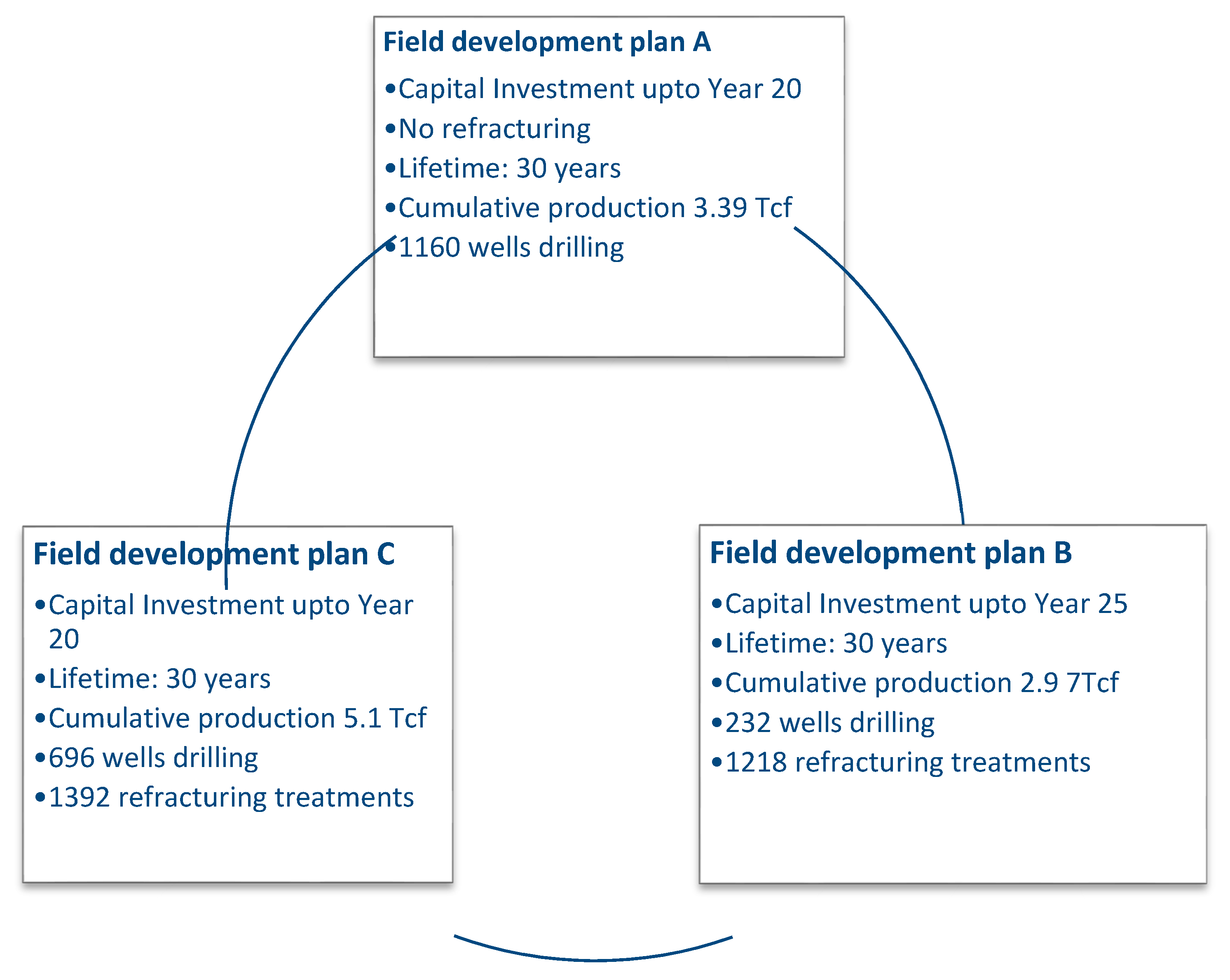
Figure 3.
Initial production rate distribution.
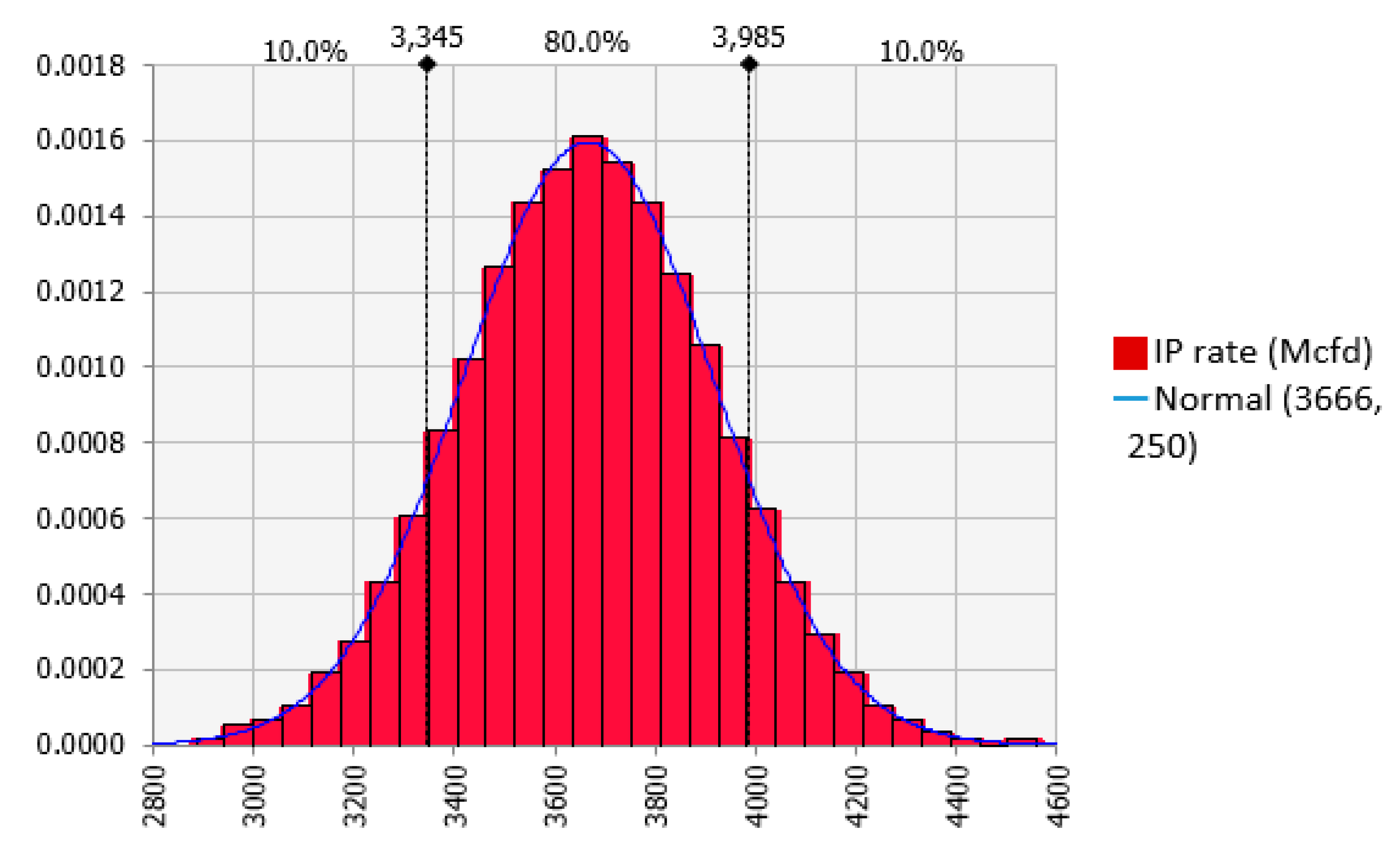
Figure 4.
Fitted hyperbolic decline.
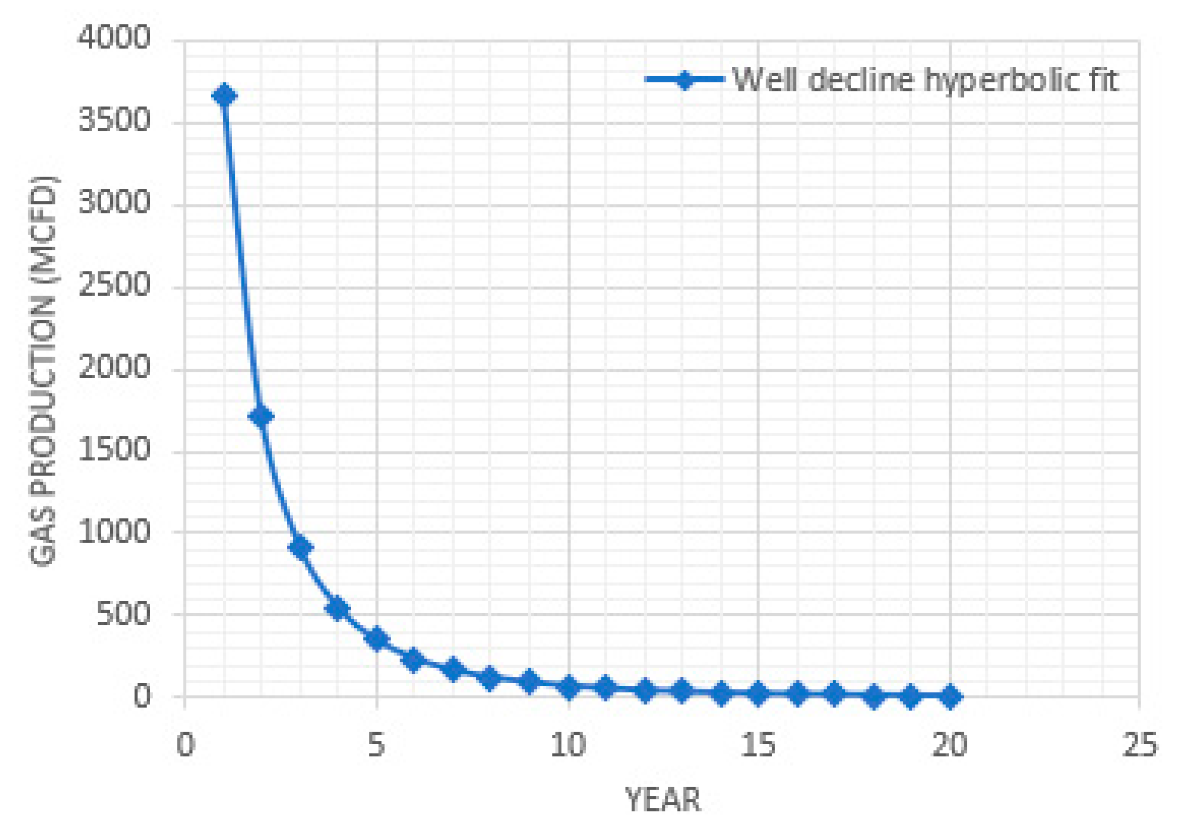
Figure 5.
Production simulation results.
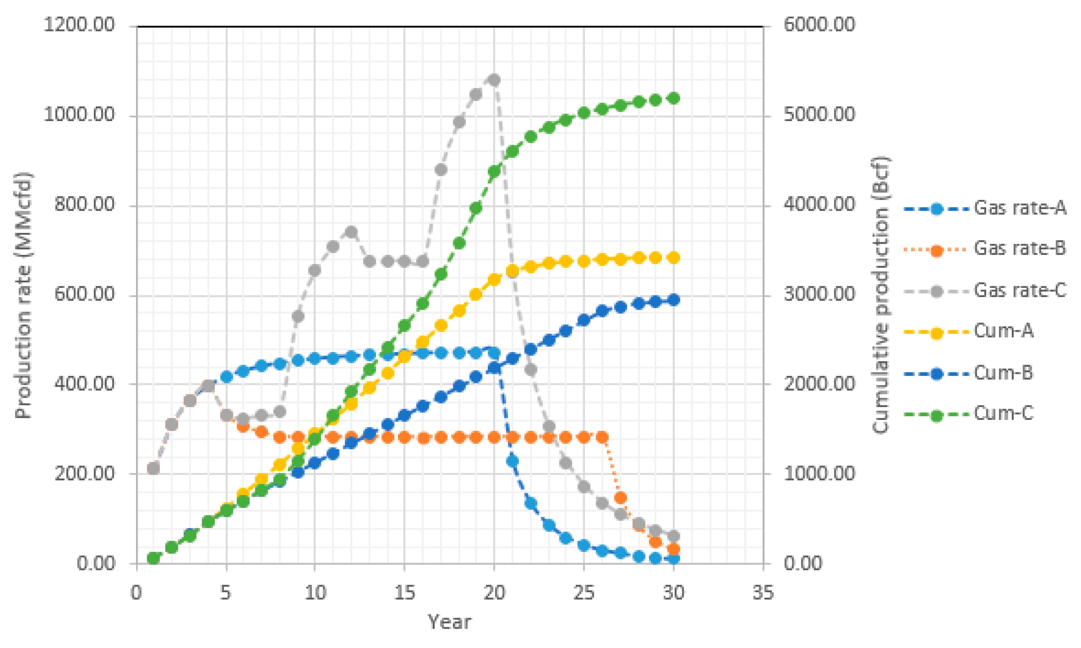
Figure 6.
Required gas price distribution for field development plan A.

Figure 7.
Required gas price distribution for field development plan B.
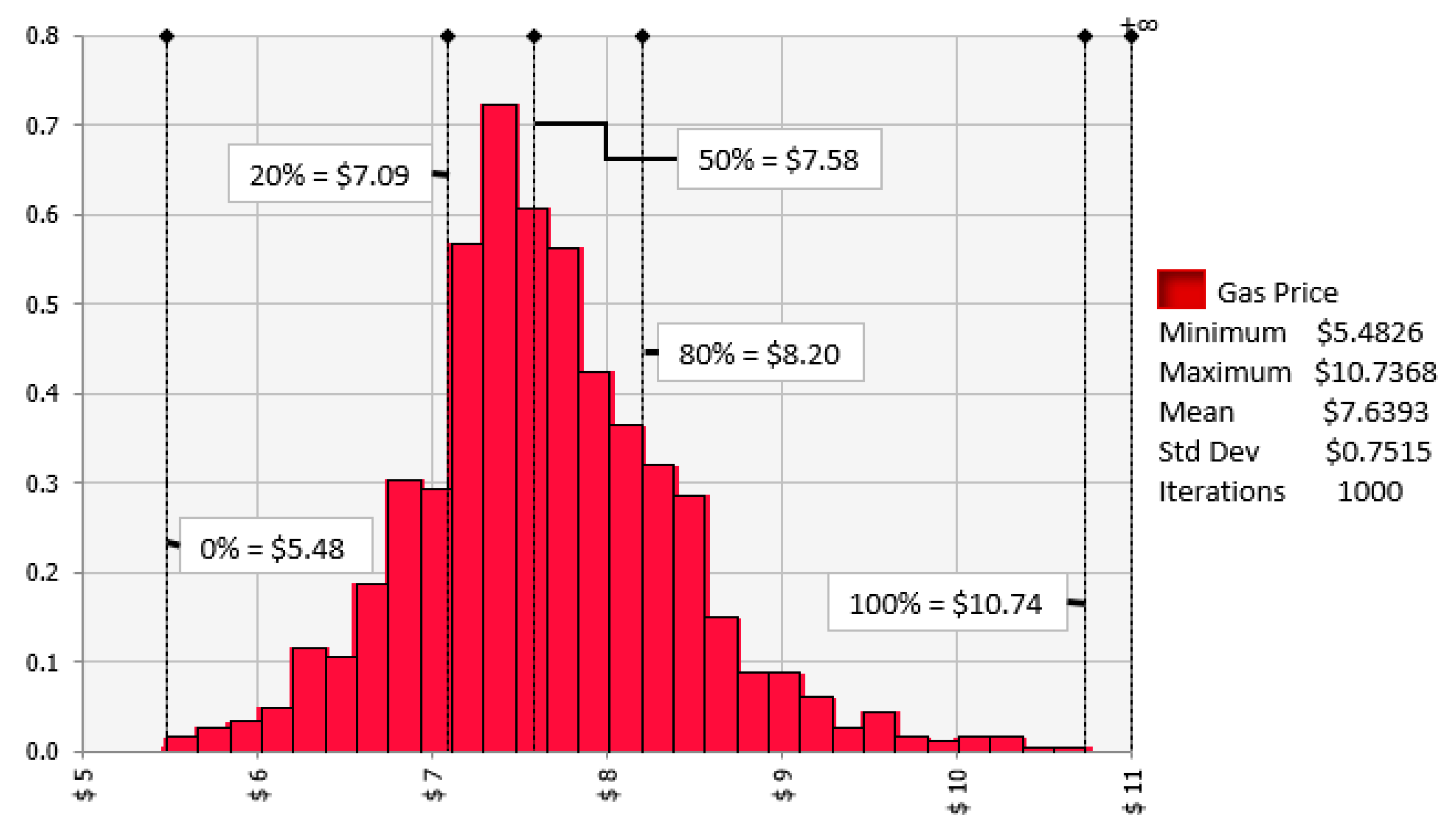
Figure 8.
Required gas price distribution for field development plan C.
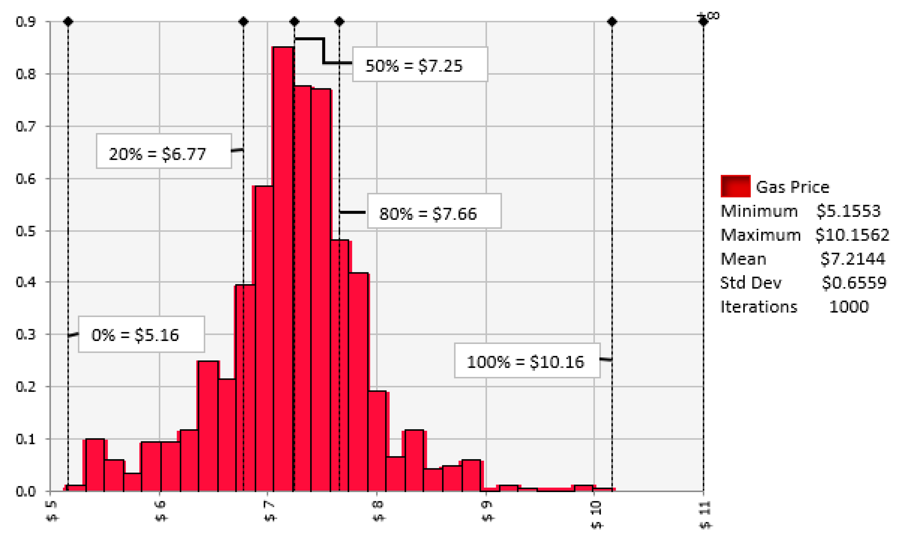
Figure 9.
Natural gas prices trend in UK (2009–2018)-dotted lines depict p80 case of development plans [46].
Figure 9.
Natural gas prices trend in UK (2009–2018)-dotted lines depict p80 case of development plans [46].
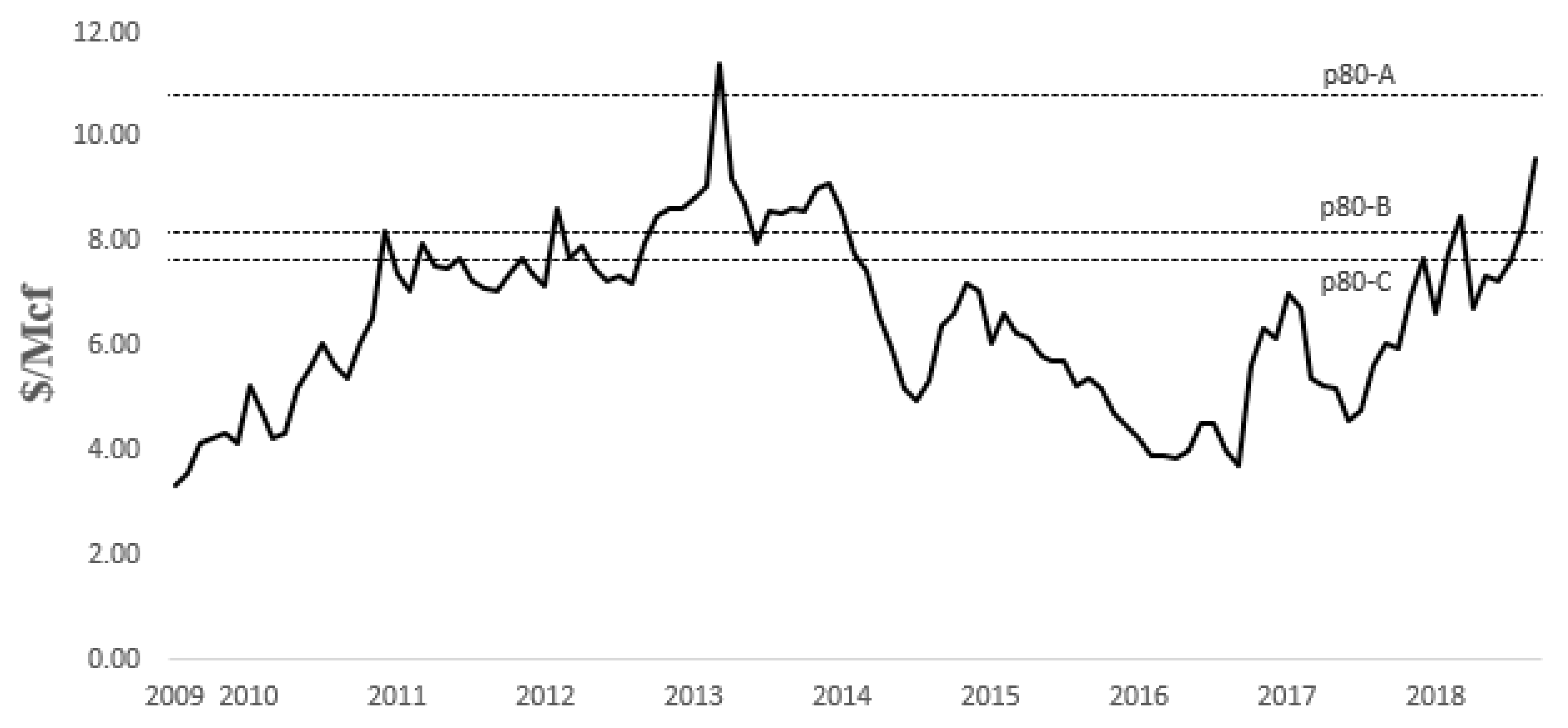
Figure 10.
Sensitivity of required gas price to ±10% variation of input parameters.


Table 1.
Geological comparison of Bowland with Barnett shale play.
| Shale Play | Barnett | Bowland |
|---|---|---|
| Age | Early Carboniferous | Late Carboniferous |
| Lithology | Siliceous mudst | Brittle shale |
| Depth (ft) | 7500 | 10,000 |
| Thickness (ft) | 300 | Over 6000 in basin centre |
| High (wt. %) | 9.94 | 8 |
| Average (wt. %) | 3.74 | 1–3 |
Table 2.
Hyperbolic decline parameters from shale gas plays of US.
| Shale Play | Case | ||
|---|---|---|---|
| Barnett | P50 | 0.869–0.9736 | 0.0212–0.244 |
| Fayetteville | P50 | 0.7372–0.9294 | 0.1011–0.3803 |
| Haynesville | P50 | 0.65501–0.96419 | 0.01153–0.52415 |
| Woodford | P50 | 0.60790–1.42630 | 0.02601–0.72473 |
| Marcellus | - | 0.90 | 0.56 |
| Eagle Ford | - | 0.77 | 0.02 |
Table 3.
Economic model input parameters.
| Variable | Unit | Distribution | Probabilistic Range | Static Value |
|---|---|---|---|---|
| Initial Production (IP) | Mcfd | Normal | Mean 3666, SD 250 | 3666 |
| Initial Decline rate | - | Normal | Mean 0.87, SD 0.07 | 0.87 |
| Decline exponent (b) | - | Triangular | T (0.01, 0.27, 1) | 0.27 |
| Well Cost (CAPEX) | $MM | Triangular | T (14, 16, 20) | 16 |
| Well Spacing | ac | - | - | 40 |
| Land Acquisition | $/ac | Uniform | 6670, 16670 | 12,000 |
| Operating Expenditure | $/Mcf | Triangular | T (1.2, 1.5, 2) | 1.5 |
| Royalty Rate | % | - | - | 12.5 |
| Ring Fence Corporation Tax (RFCT) | % | - | - | 30 |
| Supplementary Charge (SC) | % | - | - | 10 |
| Cost of Capital | % | - | - | 10 |
| Initial Production rate (refrac) | % of IP | Triangular | T (50, 70, 90) | 70 |
| Refrac Cost | $MM | Triangular | T (2, 3.5, 4) | 3.5 |
| Refrac time | Years | - | - | 4 |
Table 4.
Comparison of required gas price range for development plans.
| Field Development Plan | Mean | SD | p20 | p50 | p80 |
|---|---|---|---|---|---|
| A (only drilling) | $9.76 | $1.09 | $8.93 | $9.67 | $10.83 |
| B (only refracturing initially drilled wells) | $7.64 | $0.75 | $7.09 | $7.58 | $8.20 |
| C (new drilling, refracturing new and old wells) | $7.21 | $0.66 | $6.77 | $7.25 | $7.66 |
© 2018 by the authors. Licensee MDPI, Basel, Switzerland. This article is an open access article distributed under the terms and conditions of the Creative Commons Attribution (CC BY) license (http://creativecommons.org/licenses/by/4.0/).
Share and Cite
MDPI and ACS Style
Ahmed, M.; Rezaei-Gomari, S. Economic Feasibility Analysis of Shale Gas Extraction from UK’s Carboniferous Bowland-Hodder Shale Unit. Resources 2019, 8, 5. https://doi.org/10.3390/resources8010005
AMA Style
Ahmed M, Rezaei-Gomari S. Economic Feasibility Analysis of Shale Gas Extraction from UK’s Carboniferous Bowland-Hodder Shale Unit. Resources. 2019; 8(1):5. https://doi.org/10.3390/resources8010005
Chicago/Turabian StyleAhmed, Muhammad, and Sina Rezaei-Gomari. 2019. "Economic Feasibility Analysis of Shale Gas Extraction from UK’s Carboniferous Bowland-Hodder Shale Unit" Resources 8, no. 1: 5. https://doi.org/10.3390/resources8010005
Note that from the first issue of 2016, this journal uses article numbers instead of page numbers. See further details here.