How Spatial Analysis Can Help Enhance Material Stocks and Flows Analysis?


1
Key Lab of Urban Environment and Health, Institute of Urban Environment, Chinese Academy of Sciences, Xiamen 361021, China
2
Xiamen Key Lab of Urban Metabolism, Xiamen 361021, China
3
University of Chinese Academy of Sciences, Beijing 100049, China
*
Author to whom correspondence should be addressed.
Resources 2019, 8(1), 46; https://doi.org/10.3390/resources8010046
Submission received: 7 January 2019
/
Revised: 13 February 2019
/
Accepted: 22 February 2019
/
Published: 4 March 2019
Abstract
:Spatial information can be integrated into almost all fields of industrial ecology. Many researchers have shown that spatial proximity affects a variety of behaviors and interactions, and thus matters for materials stocks and flows analysis. However, normal tools or models in industrial ecology based on temporal dependence cannot be simply applied to the case of spatial dependence. This paper proposes a framework integrating material stocks and flows analysis with spatial analysis. We argue that spatial analysis can help data management and visualization, determine spatio-temporal patterns-processes-drivers, and finally develop dynamic and spatially explicit models, to improve the performance of simulating and assessing stocks and flows of materials. Scaling in spatial, temporal, and organizational dimensions and other current limitations are also discussed. Combined with spatial analysis, industrial ecology can really be more powerful in achieving its origin and destination—sustainability.
1. The Importance of Space in the Industrial Ecology
Most data in industry ecology are spatial data. Almost all kinds of trades, stocks, flows, processes, events, and phenomena we seek to explain in industrial ecology studies must occur at specific geographic locations. For example, research on metal trades involves multiple countries in global networks, such as a specific product’s production in China, sell and use in the USA, and final disposal in Brazil. These geographic locations are often central to our understanding of these phenomena. Many researchers have shown that spatial proximity affects a variety of trade behaviors, promotes interactions, and thus matters for material flows in the whole life cycle [1,2,3,4,5,6,7]. These are a few examples that reflect a growing interest in spatial concerns within industry ecology. It is easy to think of a myriad of additional examples that highlight the importance of geography in our lives. From good production to transportation to consumption, from metal mining through to manufacturing to use to wasting, geography has become a key conceptual and empirical concern in industrial ecology [8].
Many industrial ecologists are familiar with time-series analyses, for example, estimating in-use stocks of historical physical products in the USA from a hundred years ago [9]. However, time-series methods for modeling temporal dependence cannot simply be applied to the case of spatial dependence because the influence of temporal dependence only flows in one direction, which is from the past to the present [10]. In contrast, the diffusion of spatial dependence could affect the behavior of their neighbors and vice versa. Additionally, normal tools or models in industrial ecology usually do not take space seriously. We may collect city, regional, or country nominal variables capturing the uniqueness in particular geographic units, but rarely think of these dummy variables as spatial variables. These dummy variables merely tell us that behaviors differ for geographic units and cannot explain that the spatial dependence is consistent with diffusion or with the clustering of behaviors.
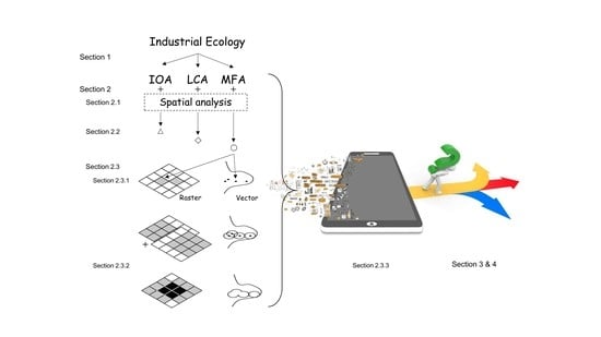
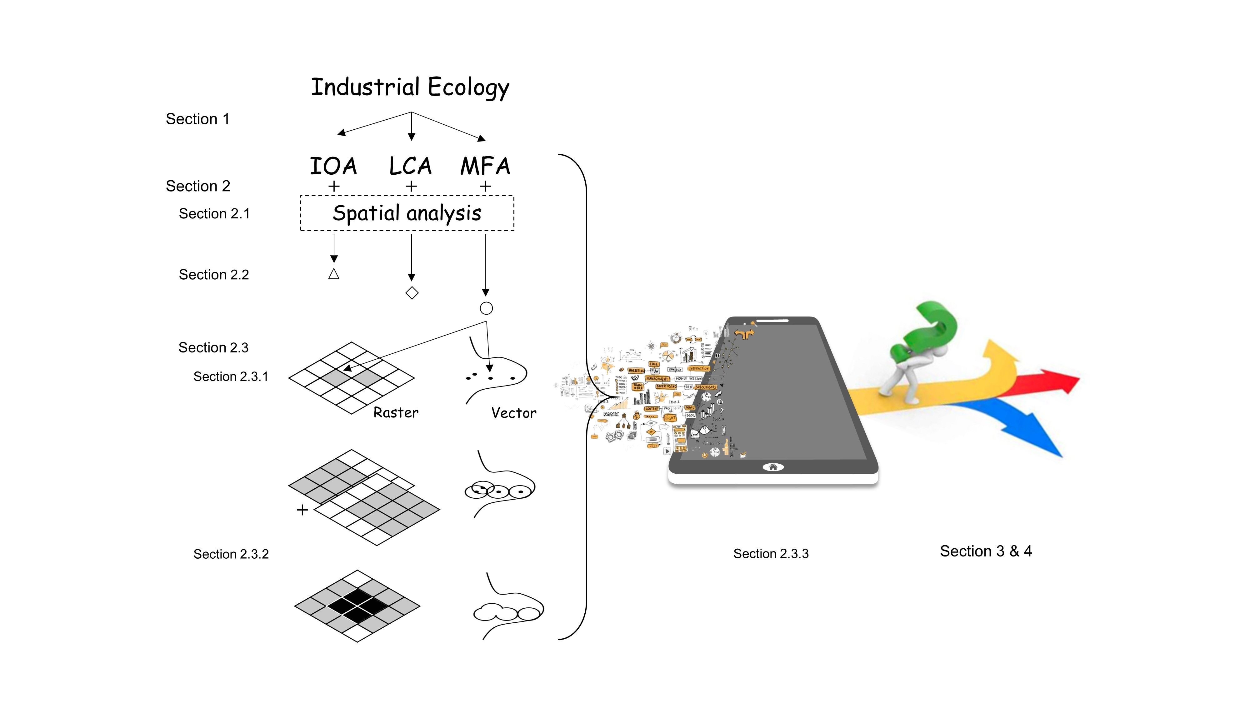
Fortunately, recent advances in spatial analysis allow us to analyze, diagnose, and model spatial dependence easily in industrial ecology. Previous reviews integrating spatial analysis into industrial ecology studies focused on specific topics in industrial symbiosis [8] and urban mining [11]. Here we further introduce the assumptions and methodologies of spatial analysis into typical tools in industrial ecology and propose a framework integrating them in detail. We provide an introduction of spatial analysis first (Section 2.1), and then try to identify the relationship between spatial information and industrial ecology tools (Section 2.2) and explain how to analyze industrial ecology topics (i.e., material stocks and flows) with spatial perspectives (Section 2.3). Three contributions were found to improve the performance of material stocks and flows analyses, they are data structure improvement (Section 2.3.1), spatial demonstration and analysis (Section 2.3.2), and finally building dynamic and spatially explicit models (Section 2.3.3) (Figure 1). In Section 3 and 4, we discuss limitations in current methods, and explore future directions (Figure 1).
2. What can Spatial Analysis Offer to Industrial Ecology?
2.1. What Is Spatial Analysis?
Spatial analysis covers any of the techniques that study entities using their topological, geometric, and geographic properties, including spatial measurement (e.g., computing length, area, or distance), overlay analysis, buffer analysis, network analysis, geostatistics (e.g., spatial autocorrelation analysis), spatial interpolation (e.g., kriging), spatial metrics (e.g., landscape metrics), and spatial simulation and modeling. Computer science, especially the geographic information system (GIS), has contributed extensively to the development of spatial analysis. There are two principal structures of spatial data that GIS works with: the raster and the vector (Figure 1). The structure of raster data is based on usually rectangular, square, or hexagon tessellation on a two dimension plane into cells (Figure 1). The size of each cell calls resolution, and the value recorded in each cell can be used to represent elements (or variables) in reality. In contrast, the structure of vector data commonly uses points, lines, and polygons to represent the shape of elements in reality (Figure 1), and the attributes of these elements can be recorded in complementary tables. Both of these data structures can encode geographical information into computer files (e.g., tiff format vs. shape format), and thus are helpful for spatializing data in industrial ecology.
2.2. What Are the Relations Between Spatial Analysis and Typical Tools Used in Industrial Ecology?
Concepts of space and geography play prominent roles in many methods and tools in industrial ecology. Meanwhile, the importance of spatial information varies among typical industrial ecology tools including input-output analysis (IOA), life cycle assessment (LCA), and material flow analysis (MFA) (Figure 1). These tools are usually used to simulate stocks and flows of materials/energy/money and to assess their environmental, social, and economic effects. IOA, as a quantitative economic model, is widely used in industrial ecology and provides material or monetary data on the intersectional flows of goods and money within an anthropogenic system [12,13]. This sectional information is highly aggregated from multi-sections and locations, unless using at very specific region (e.g., industrial park) [14]. LCA is a technique used to valuate environmental impacts associated with all stages of a product’s life cycle from raw material extraction and processing through to manufacturing, use, and finally disposal or recycling. Thus, the environmental impacts could be partially spatialized in a certain spatial scope (e.g., air pollutant emissions from a factory or waste water emits into the river nearby). MFA is an analytical method developed to quantify stocks and flows of materials or substances within an anthropogenic system on different temporal and spatial scales (e.g., city, country). On one hand, it can analyze material flows in the whole life cycle of a product. On the other hand, it can estimate material stocks and flows within a spatial context during certain life stages. For example, studying construction materials stocks and flows in the form of buildings and transportation networks in a city merely focus on the using and disposal stages of these materials. In that context, a large amount of construction materials (e.g., steel, cement) and products (e.g., air condition, television) are stored in buildings. The spatio-temporal patterns of stocks and flows can be quantified by spatial analysis according to the unique geographic location of each building. It is also an important issue in terms of understanding and managing the metabolism of socioeconomic systems. Thus, we illustrate how to combine material flow analysis with spatial analysis as an example.
2.3. Combining Material Flow Analysis with Spatial Analysis
2.3.1. Improving Data Structure
The first step before spatial analysis is changing data structure from non-spatial data to data with an explicit association relative to the location on the earth. For example, we can record buildings as polygons, roads as polylines, and manholes as points in the vector dataset with their geographic locations (Table 1). For each building or road, its attributes can be recorded in a complementary table, including area, height, structure, usage, etc. Afterwards, a city can be represented by these vectors from a bottom-up approach. All of this construction information can also be recorded into an inventory of a pixel, which is the smallest addressable element in the raster dataset (Table 1). Existing table data within an administrative entity should be identified by the locations of occurrences, such as countries, regions, cities, or administrative divisions (Table 1).
2.3.2. Spatializing Material Data
(1) Data Extrapolation and Visualization in Space
After data are matched with their geographic locations, they can be demonstrated in maps by GIS software (e.g., ArcGIS version 10.2 in Table 1). For example, data could be many points indicating pollution concentration which are collected or monitored from manufactories nearby, or many pixels representing the total stocks of metals in a city. For the first case, using a buffer analysis creates a zone around each of these points according to the distance in space (it may be helpful for evaluating the spatial influence scope), or using spatial interpolation constructs new data points and produces estimates within these known observations in space (Figure 1). The second case needs a scaling down approach to disaggregate coarse-grained information of metal stocks to spatial heterogeneity. The scaling down approach includes two complementary general approaches, including the similarity-based scaling approach and the dynamic model-based approach [23]. Similarity-based scaling methods seek scaling relations of metal stocks, for example, between city and district levels with statistical (or empirical) regressions. Dynamic model-based scaling proceed deductively with mechanism analysis and emphasize processes. For example, the total stocks of metal come from the sum of all metal products (e.g., buildings, cars, cables, electrical appliances) within a city. If we collect total numbers of these metal products and know the metal use intensity per product within each district, then the city level metal stocks can be downscaled to the district level.
(2) What Can We Do with Spatial Materials Data?
Any methods in spatial analysis can be used in material stocks and flows analysis and we demonstrate some potential pathways here. The first example is if we have several kinds of metal stocks in space and want to know where the most metal storage has. Overlay analysis can help us to answer this question by intersecting all of them (Figure 1). It also is helpful for urban mining assessment through identifying the areas with large reserves of metals and excluding the marginal areas [11]. Next, a lot of spatial metrics can be used to quantify spatial patterns of metal stocks, including spatial difference (e.g., density, similarity index, evenness index), extent (e.g., size, fractal dimension, shape complexity), fragmentation (e.g., splitting index), aggregation (e.g., aggregation index, clumpiness), diversity (e.g., Shannon’s diversity index, Simpson’s diversity index), and other composition and configuration information. Beyond describing and summarizing spatial patterns, geostatistics is helpful for determining why a specific spatial pattern exists and what processes affect this pattern. Actually, the origin of geostatistics involved trying to predict probability distributions of ore grades for mining operations [24]. Finally, we want to know why such processes operate. Analyzing and simulating direction and volume of flows and connectivity between nodes in space can be achieved by network analysis.
Based on these spatial materials data and related information on spatial patterns, processes, and feedbacks, a lot of scientific questions and practice-based queries can be answered. For example in the field of urban mining, spatial analysis helps understand dynamic character of value in recycling metals [5], trace their spatial transfer [2], and design the loop closing among recycling, remanufacturing, and waste treatment firms [25]. Environmental impacts in space can be further evaluated through carbon emissions [3,4], ecological footprint [7], teleconnecting consumption [26], or the comprehensive performance [1]. All these spatial patterns and impacts are the foundation for regional mining infrastructure planning [6] or urban diseases [27] and sustainability assessment [28].
2.3.3. Building A Dynamic and Spatially Explicit Model to Simulate Material Stocks and Flows
A dynamic and spatially explicit model finally can be established and used to represent and simulate stocks and flows of materials or substances in a city, region, country, even globe (Figure 1). The state-of-the-art models simulate and predict material stocks and flows. They can be divided into three categories based on the degree of spatial detail, including non-spatial models, quasi-spatial models, and spatially explicit models. Non-spatial models are widely used in analyzing time-series material stocks and flows [16,18,29,30,31,32,33,34,35,36,37,38]. For example, they can simulate resource demand and waste generation from a single year to a century through socioeconomic changes (e.g., economy, population, lifestyle), which is manifested in the stocks and flows of buildings and materials for their construction, demolition, and maintenance [15,36]. After establishing these components of models and their relationships in temporal perspective, another important factor in material stocks and flows is space. Spatial dynamics for many stocks and flows problems are important, because different spatial environments leading to very different patterns of stocks and contents of flows. Thus, combining MFA with GIS is proven to be an effective approach. For example, the basic function of GIS is to help visualize spatial heterogeneity of construction materials [18]. Moreover, GIS can be used to further assist construction material accounting through estimating related building parameters from remotely sensing images and georeferenced digital maps (a loose coupling approach) [20]. For a close coupling approach, GIS is treated as the data container and processor and participates whole processes in material stocks and flows analysis [21,22]. However, these state-of-the-art models coupling MFA and GIS are still quasi-spatial models due to lacks of one or more variables that are a function of space, or can be related to other spatial variables (e.g., materials exchanges between their neighbors), and we will discuss the reasons for this in the next section.
3. Limitations
3.1. Scaling
Materials and substances dynamics are generally considered complex systems because they are characterized by a large number of diverse components, nonlinear interactions, and spatial heterogeneity among multiple spatial, temporal, and organizational scales. For the first characteristic, studies in industrial ecology and other related sciences have shown that diverse components and processes tend to dominate in different dimensions of scale in time, space, and organization [1,39,40]. Traditionally, most empirical and theoretical studies in industrial ecology have been conducted over large areas and long time periods [16,41,42]. Thus, scaling down is an effective approach to extrapolate information from large areas and long time periods to small areas and short time periods. Second, nonlinear relationships and feedbacks among components exist at different scales [39,43]. For example, estimating the demolition of an individual building is difficult, because this process depends on urban planning, building’s condition, cost-benefit in economy, and residents’ willing in that building. Its demolition rate cannot be described as a logistic curve with building’s age as independence, which is usually used in evaluating demolition of buildings at urban or regional level. As Kohler and Hassler [43] said: “There is no relation between the age or condition of an individual building and the probability that it will be demolished”. Third, spatial heterogeneity varies at different scales [1,26]. For example, while metal stocks in a city can be perceived as hierarchical mosaics of patches, those patches at each spatial or temporal level may form different patterns due to variations of composition and configuration of these metals. Thus, a successful scaling strategy in industrial ecology must be able to effectively tackle these key components and complex relationships of industrial or urban systems.
3.2. Hidden Flows in Spatio-Temporal Perspectives
Even we successfully complete a scaling down approach and spatialize stocks or flows in each cell in space, it is still hard to estimate several kinds of spatial flows among cells to evolve from the quasi- to spatially explicit model. Ideally, a flow-driven and spatially explicit MFA model should describe flows among neighbors or from a place to another one (e.g., construction waste is transported from a demolishing building to a landfill). However, these flows or processes occur at daily or monthly scale and mismatch with the estimation of demolition rate at annual or decadal scales. In stock-driven models, it is easy to estimate net flows during a specific period, but usually underestimate total input and output flows because parts of flows are ignored (e.g., building replacement, repair, and maintain). All of the previously noted ineligible spatio-temporal flows and related processes finally affect accuracy in material flow analysis.
4. Conclusions and Outlooks
Many phenomena in industrial ecology studies uniquely predispose data toward spatial dependence. It is time for industrial ecologist to model the spatial dependence of material/energy stocks and flows through their whole life cycles. Here, we propose a framework integrating typical tools in industrial ecology with spatial analysis to improve the performance of materials stocks and flows analyses in both space and time (Figure 1). The simplest and most basic contribution of integrating MFA with spatial analysis is to help spatial visualization of data or results through improving their structure from non-spatial information to georeferenced maps (Table 1). Based on these spatial data, we can further quantify spatio-temporal patterns, trace processes, identify sources/sinks and hotspots, and determine drivers of material stocks and flows (Table 1). Finally, dynamic and spatially explicit models can be established and used to simulate stocks and flows of materials/energy/money in a city, country, region, even globe (Table 1).
There are still some limitations in the state-of-the-art models coupling MFA and GIS. We recognize and summarize them into three characteristics, including diverse components, nonlinear interactions, and spatial heterogeneity. Diverse components in a complex system generate hierarchical sub-systems, lead to nonlinear relationships and feedbacks, and induce various spatio-temporal patterns and processes among them.
Some detailed concerns are important for breaking above limitations and future developments of combining normal tools in industrial ecology with spatial analysis. First, the explosion of available and open data, for example business transactions, metal trades, trajectories of goods, and other big data, are geo-coded and easy to store and transmission. That advance is of great help for us to know how many materials are used or how much energy is transmitted in whole system and to understand relationships among them [17]. Second, the advances in computers and free GIS software are keeping pace with the increasing available data. Big data create considerable computational burdens for many analyzing procedures, and the burden is often greater in the spatial analysis than in the non-spatial analysis. Beyond computational capacity of computer, the challenge going forward is to develop theories and methods for using, even coupling spatial analysis into typical methods used in industrial ecology studies under the “big data” era. We all know that the origin of industrial ecology is to seek how to design sustainable industrial systems. Combining with space, industrial ecology can be much more powerful and stronger in thinking globally and acting locally.
Author Contributions
Writing—original draft preparation, Y.L.; writing—review and editing, W.-Q.C., T.L., and L.G.; funding acquisition, W.-Q.C. and Y.L.
Funding
This research was funded by National Key Research and Development Program of Ministry of Science and Technology, grant number 2017YFC0505703; National Natural Science Foundation of China, grant number 41801222; and the Key program of frontier science of the Chinese Academy of Sciences, grant number QYZDB-SSW-DQC012.
Acknowledgments
We thank the members of the Industrial and Urban Ecology group at the Institute of Urban Environment, Chinese Academy of Sciences for their suggestions on this study.
Conflicts of Interest
The authors declare no conflict of interest.
References
- Raschio, G.; Smetana, S.; Contreras, C.; Heinz, V.; Mathys, A. Spatio-Temporal Differentiation of Life Cycle Assessment Results for Average Perennial Crop Farm: A Case Study of Peruvian Cocoa Progression and Deforestation Issues. J. Ind. Ecol. 2018, 22, 1378–1388. [Google Scholar] [CrossRef]
- Sun, M.; Mao, J. Quantitative Analysis of the Anthropogenic Spatial Transfer of Lead in China. J. Ind. Ecol. 2018, 22, 155–165. [Google Scholar] [CrossRef]
- VandeWeghe, J.R.; Kennedy, C. A Spatial Analysis of Residential Greenhouse Gas Emissions in the Toronto Census Metropolitan Area. J. Ind. Ecol. 2007, 11, 133–144. [Google Scholar] [CrossRef]
- Wang, X.; Du, L. Carbon Emission Performance of China’s Power Industry: Regional Disparity and Spatial Analysis. J. Ind. Ecol. 2017, 21, 1323–1332. [Google Scholar] [CrossRef]
- Lane, R. Understanding the Dynamic Character of Value in Recycling Metals from Australia. Resources 2014, 3, 416–431. [Google Scholar] [CrossRef] [Green Version]
- Lechner, M.A.; Devi, B.; Schleger, A.; Brown, G.; McKenna, P.; Ali, H.S.; Rachmat, S.; Syukril, M.; Rogers, P. A Socio-Ecological Approach to GIS Least-Cost Modelling for Regional Mining Infrastructure Planning: A Case Study from South-East Sulawesi, Indonesia. Resources 2017, 6, 7. [Google Scholar] [CrossRef]
- Świąder, M.; Szewrański, S.; Kazak, K.J.; van Hoof, J.; Lin, D.; Wackernagel, M.; Alves, A. Application of Ecological Footprint Accounting as a Part of an Integrated Assessment of Environmental Carrying Capacity: A Case Study of the Footprint of Food of a Large City. Resources 2018, 7, 52. [Google Scholar] [CrossRef]
- Schiller, F.; Penn, A.; Druckman, A.; Basson, L.; Royston, K. Exploring Space, Exploiting Opportunities. J. Ind. Ecol. 2014, 18, 792–798. [Google Scholar] [CrossRef]
- Chen, W.Q.; Graedel, T.E. In-use product stocks link manufactured capital to natural capital. Proc. Natl. Acad. Sci. USA 2015, 112, 6265–6270. [Google Scholar] [CrossRef] [PubMed] [Green Version]
- Darmofal, D. Spatial Analysis for the Social Sciences; Cambridge University Press: Cambridge, UK; New York, NY, USA, 2015. [Google Scholar]
- Zhu, X. GIS and Urban Mining. Resources 2014, 3, 235–247. [Google Scholar] [CrossRef]
- Chen, W.Q.; Graedel, T.E.; Nuss, P.; Ohno, H. Building the Material Flow Networks of Aluminum in the 2007 U.S. Economy. Environ. Sci. Technol. 2016, 50, 3905–3912. [Google Scholar] [CrossRef] [PubMed]
- Nakamura, S.; Kondo, Y.; Kagawa, S.; Matsubae, K.; Nakajima, K.; Nagasaka, T. MaTrace: Tracing the Fate of Materials over Time and Across Products in Open-Loop Recycling. Environ. Sci. Technol. 2014, 48, 7207–7214. [Google Scholar] [CrossRef] [PubMed]
- Yang, Z.; Song, T.; Chahine, T. Spatial representations and policy implications of industrial co-agglomerations, a case study of Beijing. Habitat Int. 2016, 55, 32–45. [Google Scholar] [CrossRef] [Green Version]
- Augiseau, V.; Barles, S. Studying construction materials flows and stock: A review. Resour. Conserv. Recycl. 2017, 123, 153–164. [Google Scholar] [CrossRef]
- Canning, D. A Database of World Stocks of Infrastructure, 1950–95. World Bank Econo. Rev. 1998, 12, 529–547. [Google Scholar] [CrossRef]
- Xu, M.; Cai, H.; Liang, S. Big Data and Industrial Ecology. J. Ind. Ecol. 2015, 19, 205–210. [Google Scholar] [CrossRef]
- Han, J.; Xiang, W.-N. Analysis of material stock accumulation in China’s infrastructure and its regional disparity. Sustain. Sci. 2013, 8, 553–564. [Google Scholar] [CrossRef]
- Kleemann, F.; Lederer, J.; Rechberger, H.; Fellner, J. GIS-based Analysis of Vienna’s Material Stock in Buildings. J. Ind. Ecol. 2017, 21, 368–380. [Google Scholar] [CrossRef]
- Meinel, G.; Hecht, R.; Herold, H. Analyzing building stock using topographic maps and GIS. Build. Res. Inf. 2009, 37, 468–482. [Google Scholar] [CrossRef]
- Tanikawa, H.; Fishman, T.; Okuoka, K.; Sugimoto, K. The Weight of Society Over Time and Space: A Comprehensive Account of the Construction Material Stock of Japan, 1945–2010. J. Ind. Ecol. 2015, 19, 778–791. [Google Scholar] [CrossRef]
- Tanikawa, H.; Hashimoto, S. Urban stock over time: spatial material stock analysis using 4d-GIS. Build. Res. Inf. 2009, 37, 483–502. [Google Scholar] [CrossRef]
- Wu, J. Hierarchy and scaling: Extrapolating information along a scaling ladder. Can. J. Remote Sens. 1999, 25, 367–380. [Google Scholar] [CrossRef]
- Armstrong, M.; Champigny, N. A study on kriging small blocks. Cim. Bulletin 1989, 82, 128–133. [Google Scholar]
- Lyons, D.I. A Spatial Analysis of Loop Closing Among Recycling, Remanufacturing, and Waste Treatment Firms in Texas. J. Ind. Ecol. 2007, 11, 43–54. [Google Scholar] [CrossRef]
- Hubacek, K.; Feng, K.; Minx, J.C.; Pfister, S.; Zhou, N. Teleconnecting Consumption to Environmental Impacts at Multiple Spatial Scales. J. Ind. Ecol. 2014, 18, 7–9. [Google Scholar] [CrossRef]
- Saravanan, V.S.; Mavalankar, D.; Kulkarni, S.P.; Nussbaum, S.; Weigelt, M. Metabolized-Water Breeding Diseases in Urban India: Sociospatiality of Water Problems and Health Burden in Ahmedabad City. J. Ind. Ecol. 2015, 19, 93–103. [Google Scholar] [CrossRef]
- Wu, S.R.; Li, X.; Apul, D.; Breeze, V.; Tang, Y.; Fan, Y.; Chen, J. Agent-Based Modeling of Temporal and Spatial Dynamics in Life Cycle Sustainability Assessment. J. Ind. Ecol. 2017, 21, 1507–1521. [Google Scholar] [CrossRef] [Green Version]
- Bergsdal, H.; Brattebø, H.; Bohne, R.A.; Müller, D.B. Dynamic material flow analysis for Norway’s dwelling stock. Build. Res. Inf. 2007, 35, 557–570. [Google Scholar] [CrossRef]
- Hu, D.; You, F.; Zhao, Y.; Yuan, Y.; Liu, T.; Cao, A.; Wang, Z.; Zhang, J. Input, stocks and output flows of urban residential building system in Beijing city, China from 1949 to 2008. Resour. Conserv. Recycl. 2010, 54, 1177–1188. [Google Scholar] [CrossRef] [Green Version]
- Hu, M.; Bergsdal, H.; van der Voet, E.; Huppes, G.; Müller, D.B. Dynamics of urban and rural housing stocks in China. Build. Res. Inf. 2010, 38, 301–317. [Google Scholar] [CrossRef] [Green Version]
- Hu, M.; Voet, E.V.D.; Huppes, G. Dynamic Material Flow Analysis for Strategic Construction and Demolition Waste Management in Beijing. J. Ind. Ecol. 2010, 14, 440–456. [Google Scholar] [CrossRef]
- Huang, C.; Han, J.; Chen, W.-Q. Changing patterns and determinants of infrastructures’ material stocks in Chinese cities. Resour. Conserv. Recycl. 2017, 123, 47–53. [Google Scholar] [CrossRef]
- Huang, T.; Shi, F.; Tanikawa, H.; Fei, J.; Han, J. Materials demand and environmental impact of buildings construction and demolition in China based on dynamic material flow analysis. Resour. Conserv. Recycl. 2013, 72, 91–101. [Google Scholar] [CrossRef]
- Miatto, A.; Schandl, H.; Wiedenhofer, D.; Krausmann, F.; Tanikawa, H. Modeling material flows and stocks of the road network in the United States 1905–2015. Resour. Conserv. Recycl. 2017, 127, 168–178. [Google Scholar] [CrossRef]
- Müller, D. Stock dynamics for forecasting material flows—Case study for housing in The Netherlands. Ecolo. Econ. 2006, 59, 142–156. [Google Scholar] [CrossRef]
- Wiedenhofer, D.; Steinberger, J.K.; Eisenmenger, N.; Haas, W. Maintenance and Expansion: Modeling Material Stocks and Flows for Residential Buildings and Transportation Networks in the EU25. J. Ind. Ecol. 2015, 19, 538–551. [Google Scholar] [CrossRef] [PubMed] [Green Version]
- Yang, W.; Kohler, N. Simulation of the evolution of the Chinese building and infrastructure stock. Build. Res. Inf. 2008, 36, 1–19. [Google Scholar] [CrossRef]
- Caduff, M.; Huijbregts, M.A.J.; Koehler, A.; Althaus, H.-J.; Hellweg, S. Scaling Relationships in Life Cycle Assessment. J. Ind. Ecol. 2014, 18, 393–406. [Google Scholar] [CrossRef]
- Patrício, J.; Kalmykova, Y.; Rosado, L.; Lisovskaja, V. Uncertainty in Material Flow Analysis Indicators at Different Spatial Levels. J. Ind. Ecol. 2015, 19, 837–852. [Google Scholar] [CrossRef]
- Rauch, J.N. Global mapping of Al, Cu, Fe, and Zn in-use stocks and in-ground resources. Proc. Natl. Acad. Sci. USA 2009, 106, 18920–18925. [Google Scholar] [CrossRef] [PubMed] [Green Version]
- Van Ewijk, S.; Stegemann, J.A.; Ekins, P. Global Life Cycle Paper Flows, Recycling Metrics, and Material Efficiency. J. Ind. Ecol. 2017, 22, 686–693. [Google Scholar] [CrossRef] [Green Version]
- Kohler, N.; Hassler, U. The building stock as a research object. Build. Res. Inf. 2002, 30, 226–236. [Google Scholar] [CrossRef] [Green Version]
Figure 1.
A framework of combining material flow analysis with spatial analysis.


Table 1.
The different roles of data structures in material flow analysis.
| Data Structures | Table (e.g., for Each Administrative Entity) | Grid | Vector | References | |
|---|---|---|---|---|---|
| Analysis Processes | Data sources | *** | ** | ** | [15,16,17] |
| Data/results demonstration | ** | *** | *** | [11,18] | |
| Spatial analyzing/modelling | * | *** | *** | [8,11,15,19,20,21,22] | |
* rare; ** common; *** popular.
© 2019 by the authors. Licensee MDPI, Basel, Switzerland. This article is an open access article distributed under the terms and conditions of the Creative Commons Attribution (CC BY) license (http://creativecommons.org/licenses/by/4.0/).
Share and Cite
MDPI and ACS Style
Liu, Y.; Chen, W.-Q.; Lin, T.; Gao, L. How Spatial Analysis Can Help Enhance Material Stocks and Flows Analysis? Resources 2019, 8, 46. https://doi.org/10.3390/resources8010046
AMA Style
Liu Y, Chen W-Q, Lin T, Gao L. How Spatial Analysis Can Help Enhance Material Stocks and Flows Analysis? Resources. 2019; 8(1):46. https://doi.org/10.3390/resources8010046
Chicago/Turabian StyleLiu, Yupeng, Wei-Qiang Chen, Tao Lin, and Lijie Gao. 2019. "How Spatial Analysis Can Help Enhance Material Stocks and Flows Analysis?" Resources 8, no. 1: 46. https://doi.org/10.3390/resources8010046
Note that from the first issue of 2016, this journal uses article numbers instead of page numbers. See further details here.