1. Introduction
Mountains play an important role in the Earth System and the availability of water resources. They cover 25% of the global land surface, provide living space for 26% of the world’s population [
1,
2], supply freshwater resources to surrounding lowlands, and host a significant amount of biodiversity. Mountain environments are highly sensitive to changes in climate [
3] and are sensors for early detection of climate change [
4]. The high sensitivity of mountain environments to climate change has generated significant research to improve climate observations at high elevations [
5]. The alpine regions of the Mediterranean are among the most climatically sensitive areas in the world [
6]. In many areas of the world, climate monitoring in high altitude regions continues to be sparse and of low quality; observation networks are deficient and climate values are estimated by extrapolating from low-altitude data. This can be particularly misleading when extrapolating precipitation. There appears to be a general positive correlation between precipitation and altitude [
7,
8], but it is not as simple and direct as the high (negative) correlation between temperature and altitude [
9,
10].
The focus of the work presented here is a study on the spatio-temporal dynamics of precipitation and temperature in the high-altitude Sierra Nevada mountain range in Southern Spain in order to evaluate the spatio-temporal dynamics of water resources in the form of rainfall and snow. There have been many studies on precipitation in Southern Spain. For example, various aspects of precipitation in the Mediterranean region of Spain are considered in [
11,
12]. The authors of [
13] studied daily precipitation in Spain for the period of 1951 to 2002 using data from 22 sites. The authors of [
14] studied seasonal trends in precipitation in the Mediterranean Iberian peninsula from 1951 to 2000. The authors of [
15] studied dry periods over the pluviometric gradient (from Gibraltar to Almeria) in Mediterranean southern Spain. The authors of [
16] provided a database of gridded precipitation and temperature in Spain for the 1950–2003 period, but the grid spacing they used had a horizontal resolution of approximately 20 km.
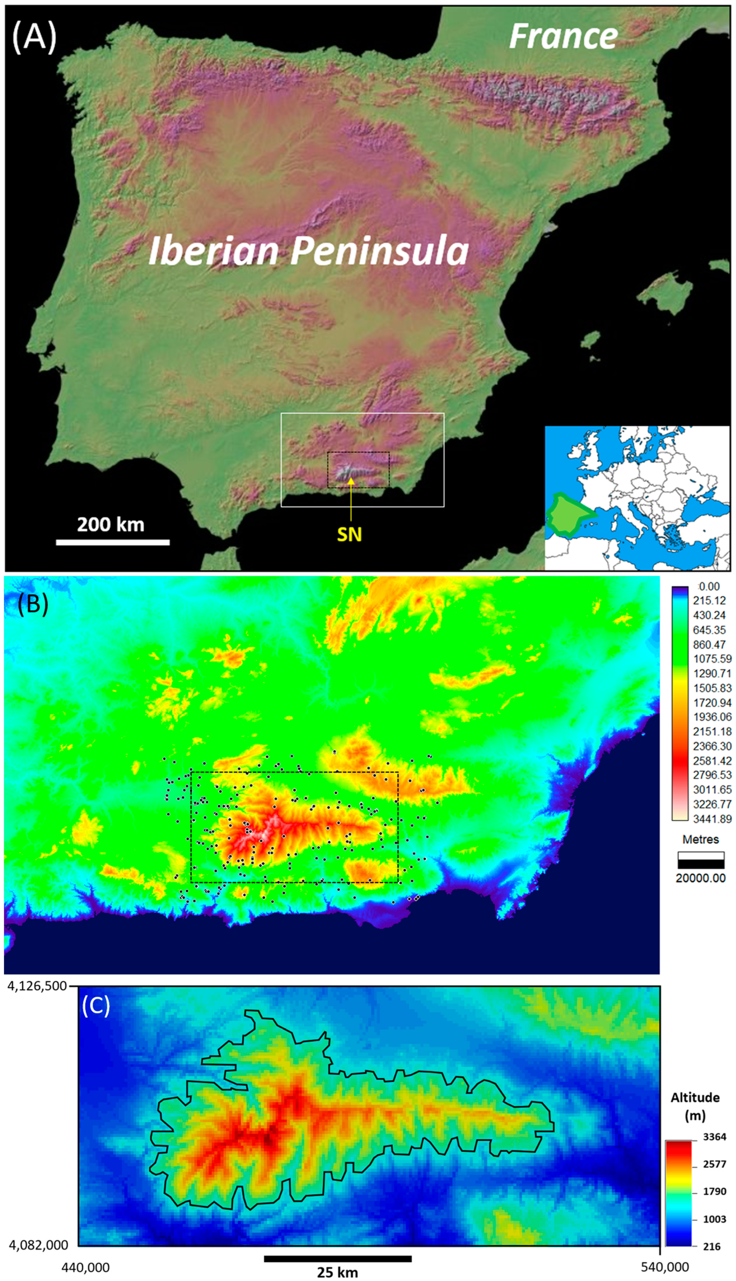
These and other previous studies have estimated precipitation and temperature over large regions, such as the entire Mediterranean region or the whole of the Iberian Peninsula, without any altitudinal restriction. The work presented here focuses on precipitation and temperature within the high-altitude area of the Sierra Nevada mountain range, and specifically, on the connected region with altitudes from 1500 m above sea level (asl) to almost 3500 m asl, which comprises the most southern alpine environment in Europe. The objective was to build a database of daily precipitation and temperature within this high-altitude area and to interpret it by using various statistical analyses, as explained in the following sections. This database reveals the spatio-temporal evolution of water resources in the studied area.
2. Methodology
Estimating precipitation in mountainous areas is a problem of recent interest [
17,
18]. There are particular solutions to the general problem of evaluating the areal distribution of precipitation using limited precipitation records (see for example [
19,
20] for urban areas). However, geostatistics has proved to be the optimal technique for estimating daily precipitation and daily temperature using altitude as a secondary variable [
21,
22,
23], among others. Altitude data are readily available from digital elevation models (DEMs) which provide complete coverage of an area. Rainfall data, however, are limited to sparsely located rain gauges. Temperature data are even more sparse, although they show a higher (negative) correlation with altitude. There are various geostatistical kriging procedures for incorporating altitude as a secondary variable. The most widely used is co-kriging [
24], which is a multivariate geostatistical interpolator [
25]. Essentially, the relative scarcity of the directly measured data for the primary variable (precipitation or temperature) is compensated for by using its spatial correlation with the more abundant secondary variable (altitude). The application of co-kriging requires estimates of the direct variogram (or covariance) of precipitation (or temperature), the direct variogram (or covariance) of altitude, and the cross-variogram (or cross-covariance) of precipitation and altitude (or temperature and altitude). These three estimated variograms are modelled by fitting permissible models, of which the most widely used is the linear co-regionalisation model [
26]. Co-kriging is used to estimate daily precipitation and temperature on a regular grid, and seasonal and annual averages are estimated by summing the days contained in the chosen time period (or support in geostatistical terminology) of estimation (e.g., one month, one season, one year). As the number of rain gauges and temperature stations available for any particular day may be small, a climatological variogram is used [
27,
28]. The shape and range of the climatological variogram remains constant, while the nugget variance and partial sill are updated with daily precipitation and temperature statistics [
28]. The mathematical basics of co-kriging are considered next.
Co-kriging is a geostatistical method for optimal multivariate spatial interpolation [
26]. In geostatistics, spatial variable
at spatial location
, representing, for example rainfall, minimum temperature, maximum temperature, etc., is modelled as a random variable. The set of all random variables
in region
of the space,
, comprises a random function or random field
. With
and
, the problem is two-dimensional, as is the case in the work presented here for precipitation or temperature and elevation. Thus,
represents precipitation or temperature and is the variable of interest that is to be estimated by co-kriging.
It is assumed that
is second-order stationary with constant spatial mean
and the two-point statistics, the covariance, and the variogram functions depend only on vector
:
where
and
are, respectively, the mean, variance, variogram, and covariance of the random function
and
is the mathematical expectation operator.
In the simplest form of co-kriging, a variable of interest, or primary variable (e.g., temperature or precipitation), is estimated based on the experimental values of the variable and the experimental values of a secondary variable (e.g., altitude) that is correlated with the primary variable. The co-kriging estimator of the precipitation (or temperature) at any given geographical location
, where
are the easting and northing coordinates respectively, can be expressed as:
where:
is the primary variable, precipitation or temperature, at location , and is the secondary variable, altitude, at location .
and are the number of values of variables and , respectively, used in the estimation in Equation (5). Usually, these data are inside a neighbourhood centred on estimation location .
The optimal weights for the linear estimation in Equation (5) are obtained by solving the corresponding co-kriging system; see for example, refs. [
25,
29]. If only the primary variable is used, ordinary co-kriging reduces to ordinary kriging of the primary variable. The same applies if there is no correlation between the primary and secondary variables.
For co-kriging, the direct variograms of the two variables and the cross-variogram (or direct covariances and cross-covariance) between the two variables must be estimated from the experimental data.
The unbiasedness of the co-kriging estimator in Equation (5) implies that the mean estimation error is zero:
This is achieved by including the following conditions in the co-kriging system:
and
The variance of the estimation error can be written as:
The co-kriging system is obtained by minimising the estimated variance in Equation (1), subject to the unbiasedness conditions, which, in matrix form [
30], is:
with:
where
and
are Lagrange multipliers or parameters that are used to include the constraints given in Equations (7) and (8).
The solution of the co-kriging system:
provides the weights required in the estimator in Equation (5).
In the geostatistical literature, the form of co-kriging summarised above is known as “ordinary co-kriging” to distinguish it from “simple co-kriging”, in which the mean
in Equation (1) is known [
26,
29,
31].
4. Results
Geostatistical co-kriging was applied to the database of experimental precipitation and temperature data. The linear regionalisation model was used with a spherical variogram model with a range of 30 km and a nugget variance and partial sill that were updated each day according to the daily variance of precipitation and temperature, i.e., following the methodology of the climatological variogram. The result is a new database comprising daily precipitation and temperature (minimum, maximum and mean) for 67 years on a 500 m × 500 m spatial grid (
Figure 1C).
Using the new database, various averages in space and time can be calculated to highlight the spatio-temporal dynamics of precipitation and temperature for the Sierra Nevada mountain range. As shown in
Figure 1C, the mountain range has been defined by including all points of the estimation grid that have an altitude greater than 1500 m and that yield a connected polygon that clearly defines the Sierra Nevada mountain range.
The first important result is the mean annual precipitation in the Sierra Nevada for the period from 1951 to 2017, which is represented in
Figure 3.
Figure 3A shows a raster colour map and
Figure 3B shows lines of equal precipitation (isohyets) overlaying the raster DEM in
Figure 1C. The most surprising result is the strong orographic influence in the spatial distribution of the mean annual precipitation. The most striking fact is that the dome of maximum precipitation has an NW–SE orientation rather than the E–W main topographical orientation of the Sierra Nevada orographic dome, as reported in most previous studies. The second interesting result is that the maximum coincides with the summit of the range but is in the upper part of the main valley of the southern slope. The third surprising result is that there is a second relative maximum (2 in
Figure 3A) in the eastern part of the Sierra, also located on the southern slope. There is also a second maximum of annual rainfall (3 in
Figure 3A), but it is located outside, and northwest of, the Sierra Nevada mountain range.
The estimated map of mean annual precipitation (
Figure 3A) is consistent with Figure 2 of Sumner et al. (2003) [
32], which represents the average annual precipitation (mm) for 1964–1993, but not with the detail given in the work presented here. In addition, the Confederación Hidrográfica del Guadalquivir (Water authority for the management of the Guadalquivir river basin) reported a mean precipitation of 618 mm in the river basin of the Canales dam (with a surface of 176 km
2). A similar estimate of 633 mm was obtained for the areal value for the same river basin in the map in
Figure 3A.
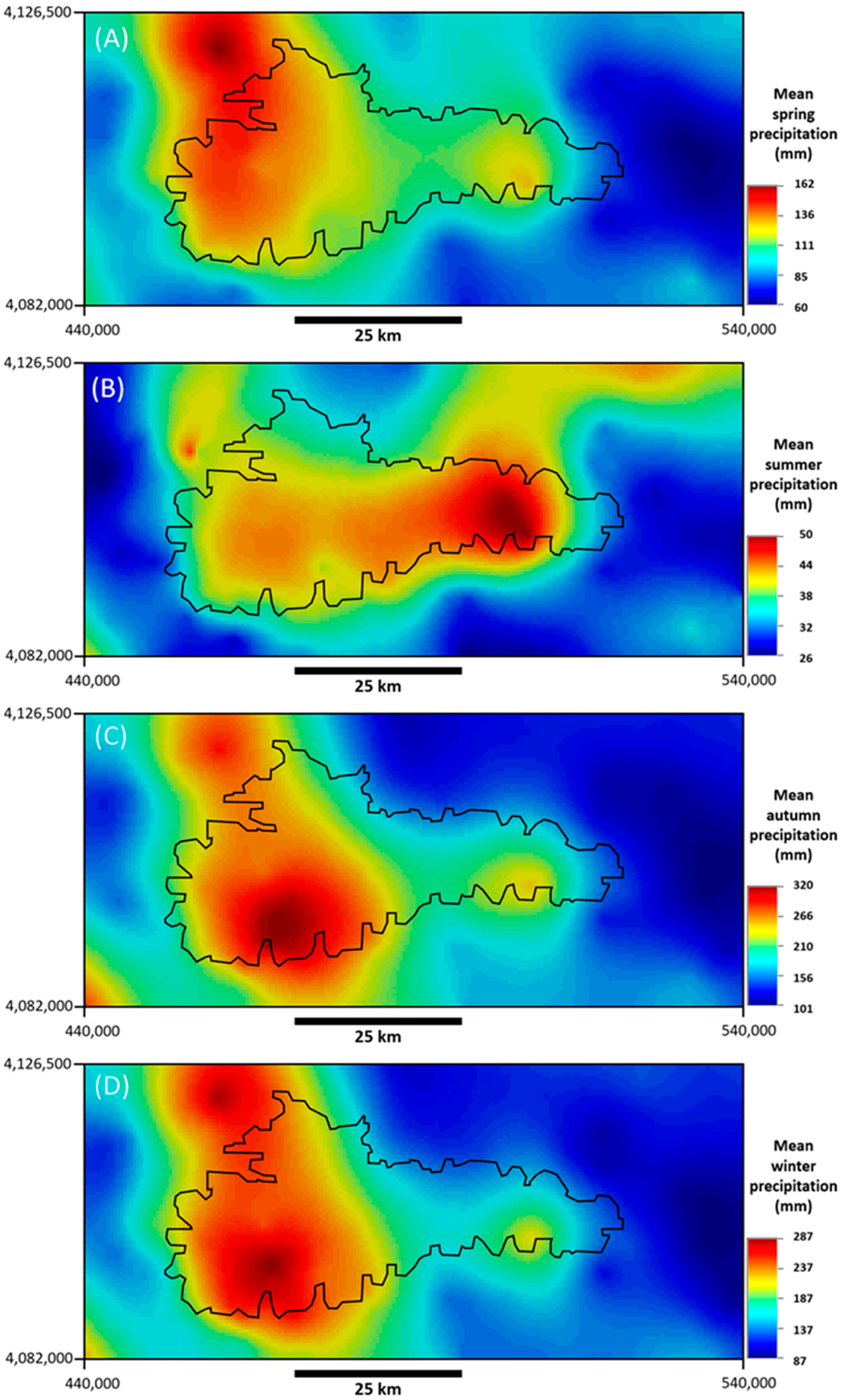
Another interesting result is the map of mean precipitation for the 1951–2017 period, but instead of integrating time for the year, it is integrated for each season: Spring (April, May, June), Summer (July, August, September), Autumn (October, November, December), and Winter (January, February, March). The results are shown in
Figure 4 and can be interpreted as a decomposition of the mean annual precipitation in
Figure 3 to produce the mean precipitation by season. This map should be assessed in conjunction with the results shown in
Table 1, which shows the mean precipitation by month and season.
Table 1 shows that, climatologically, the driest month is July, with less than 1% of the annual precipitation, while the wettest month is December, with 15% of the yearly precipitation. August is also a dry month, with 1.2% of the annual precipitation, while June and September, with 3.1% and 4.9% respectively of the annual precipitation, can be considered intermediate months. The remaining months, from October to May, can be considered humid months that define the rainy season. The seasons, from wettest to driest, are Autumn, Winter, Spring and Summer, with 39%, 34%, 20% and 7% respectively of the annual precipitation. The mean annual precipitation for Sierra Nevada for the 1951–2017 period is 575 mm with a standard deviation of 191 mm; this implies a high variability from year to year.
Figure 4 shows that the wettest seasons (Autumn in
Figure 4C and Winter in
Figure 4D) reproduce the annual mean precipitation shown in
Figure 3. The general spatial trend of the annual precipitation in
Figure 3 is also reproduced in the other two seasons (Spring and Summer) but with the difference that the maximum precipitation in Spring occurred outside the target area in the north-western sector (number 3 in
Figure 3A), while the maximum precipitation in Summer occurred in the second maximum of precipitation inside the target area, located in the eastern part of the Sierra (number 2 in
Figure 3A). This behaviour was due to the orographic effect and the provenance of the humid winds, as explained in the discussion section.
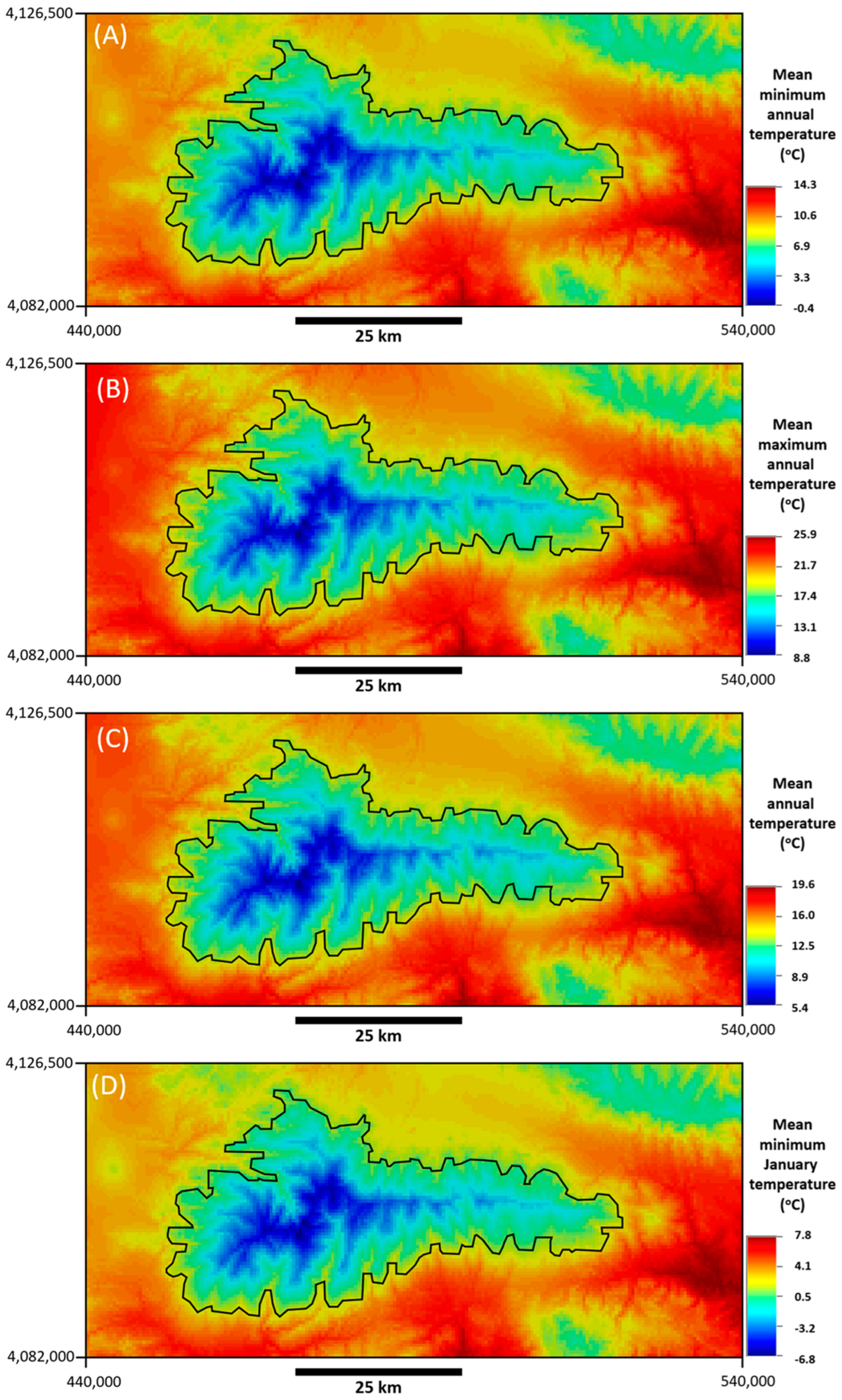
Another important result is the mean annual temperature (minimum, maximum, and mean) in the Sierra Nevada for the period from 1951 to 2017, which is represented in
Figure 5A–C, respectively. Because of the high negative correlation between temperature and altitude, the temperature maps in
Figure 5 clearly resemble the map of altitudes in
Figure 1C. The spatial distribution of temperatures can be calculated for any temporal interval as, for example, in
Figure 5D, which shows the minimum January temperature for the 1951–2017 period.
Figure 6A shows the spatial variability of the total annual snow obtained by assuming that the daily precipitation when the minimum daily temperature was below zero degrees Celsius would fall in the form of snow.
Figure 6B shows that the percentage of total precipitation that fell in the form of snow increased with altitude and, within the Sierra Nevada mountain range, varied from 4.2% to 78.7%, with a mean of 24.9%.
Another interesting result is the time series of the areal average of the annual precipitation for Sierra Nevada (black polygon in
Figure 1C) for the 1951–2017 period, i.e., a period of 67 years or almost seven decades. The estimated time series is shown in
Figure 7A. The mean annual precipitation of 575 mm is represented as a horizontal, large-dashed line. The high variability of annual precipitation over the years is reflected in a time series with a standard deviation of 191 mm. Despite this high variability, the annual precipitation decreased linearly at a rate of 33 mm of precipitation per decade. The negative slope is statistically significant (i.e., differs from zero), with a confidence level of 95%. The fitted linear trend is shown as a solid red line in
Figure 7A. This decrease can be seasonally decomposed as a decrease of 15 mm in Winter precipitation, 12 mm in Autumn precipitation, and 6 mm in Spring precipitation, while there was no significant change in Summer precipitation. In addition, the years with the lowest precipitation coincided with droughts in southern Spain or in the entire Iberian Peninsula and have been marked with blue arrows in
Figure 7A. It is clear from the Figure that the number of droughts increased with time, and it is estimated that a mean precipitation in Sierra Nevada of less than 440 mm is indicative of a drought in the region. A different aspect is the evolution of seasonality, defined here as the percentage of annual precipitation comprising Autumn precipitation. The result is shown in
Figure 7B, in which it is clear that seasonality has remained unchanged over the 1951–2017 period. Seasonality has been defined as the percentage of annual precipitation occurring in Autumn, because Autumn is the main wet season in the area, recording, on average, 40% of the precipitation of the whole year.
Although
Figure 7A shows the time series of the mean total rainfall over the Sierra Nevada mountain range, the same time series can be calculated on a pixel basis to show the spatial variability of the slope of the total rainfall as in
Figure 8A. It can be seen that inside the Sierra Nevada limits, the slope is always negative (rainfall decreasing with time), but it is statistically significant (at the 95% confidence level) in the western part and on the northern side of the eastern part.
A spectral analysis of the time series of mean annual precipitation may reveal hidden periodicities or cycles in precipitation. The maximum entropy method [
33,
34] was applied to the time series in
Figure 7A and the estimated power spectrum is shown in
Figure 9. There are important cycles lasting around 12 years, related to sunspot cycles. A cycle of 83 years is also related to solar activity but is less reliable because it is longer than the length of the time series of the available data. The cycles of 6.5, 3.4, and 2.7 years are related to the North Atlantic Oscillation (NAO) index.
The previous suggestion that there may be a relationship between annual precipitation and the annual NAO index has been investigated further. Both variables (annual precipitation and the annual NAO index) are plotted in
Figure 10A, in which there is an obvious correspondence of wet years with a negative NAO index, whereas dry years are related to a positive NAO index. This negative relationship can be more clearly seen by comparing the polynomial trends fitted to both time series (thick solid line in
Figure 10A). This clear relationship between precipitation in the Sierra Nevada and the NAO index is considered further in the discussion section, as is the issue of the altitudinal precipitation gradient.
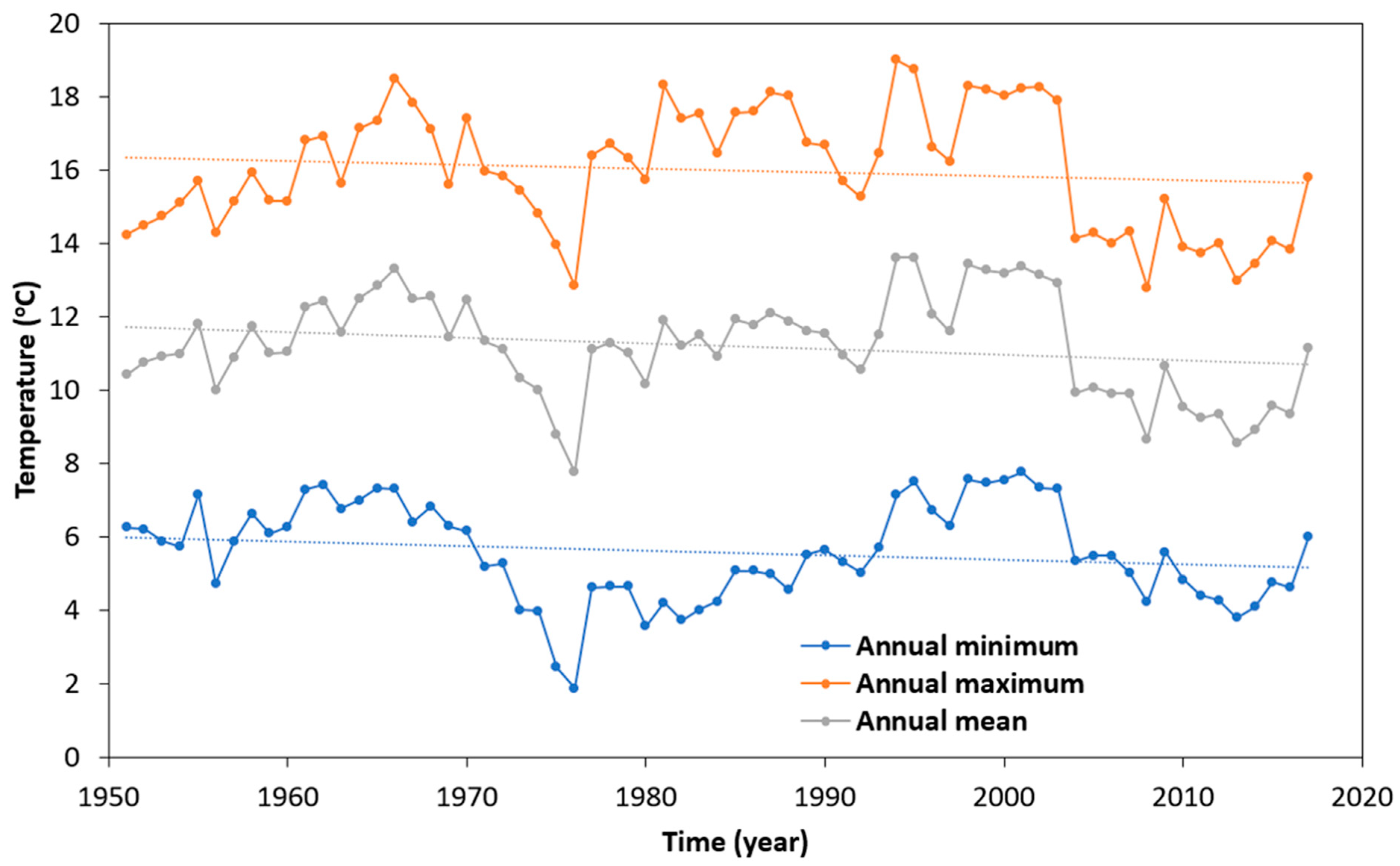
With respect to temperature,
Figure 11 shows, for the Sierra Nevada mountain range, the time series of minimum, maximum, and mean temperatures for the 1951–2017 period. It is clear from the figure that the slope is negative, which implies that temperature is decreasing at a rate of around 0.1 °C every 10 years, which seems paradoxical in a global warming context. However, it can be shown that all three slopes are statistically significant with a confidence level of 95%. Again, it is instructive to assess the time series of the different temperatures for the different pixels, i.e., the spatial variability of the trend across space, as shown in
Figure 12.
Figure 12A shows minimum temperature,
Figure 12C shows maximum temperature, and
Figure 12B,D shows the statistical significance of the different slopes. For both minimum and maximum temperatures, there are positive and negative trends, together with areas that are not statistically significant (at the 95% confidence level), areas that have positive slopes that are statistically significant, and areas that have negative slopes that are statistically significant. For both minimum and maximum temperatures, the statistically significant positive slopes (increasing temperature with time) are in the eastern part of the mountain range, while the statistically significant negative slopes (decreasing temperature) are in the western part of the mountain range.
Finally, the equivalent product for snow can be obtained by using a simple snow precipitation and melting model. The adopted model is precipitation in the form of snow when the minimum temperature is below zero degrees Celsius. The melting model used is the temperature index of the snow melt model [
35], formulated as:
where
are the daily minimum, maximum, and mean temperature, respectively.
: is the cell with spatial location (i, j) for day (t).
are real numbers. The first two are temperature thresholds and the third is a multiplicative melting factor.
The parameters were selected using a simple calibration that gave the following: , , , , and .
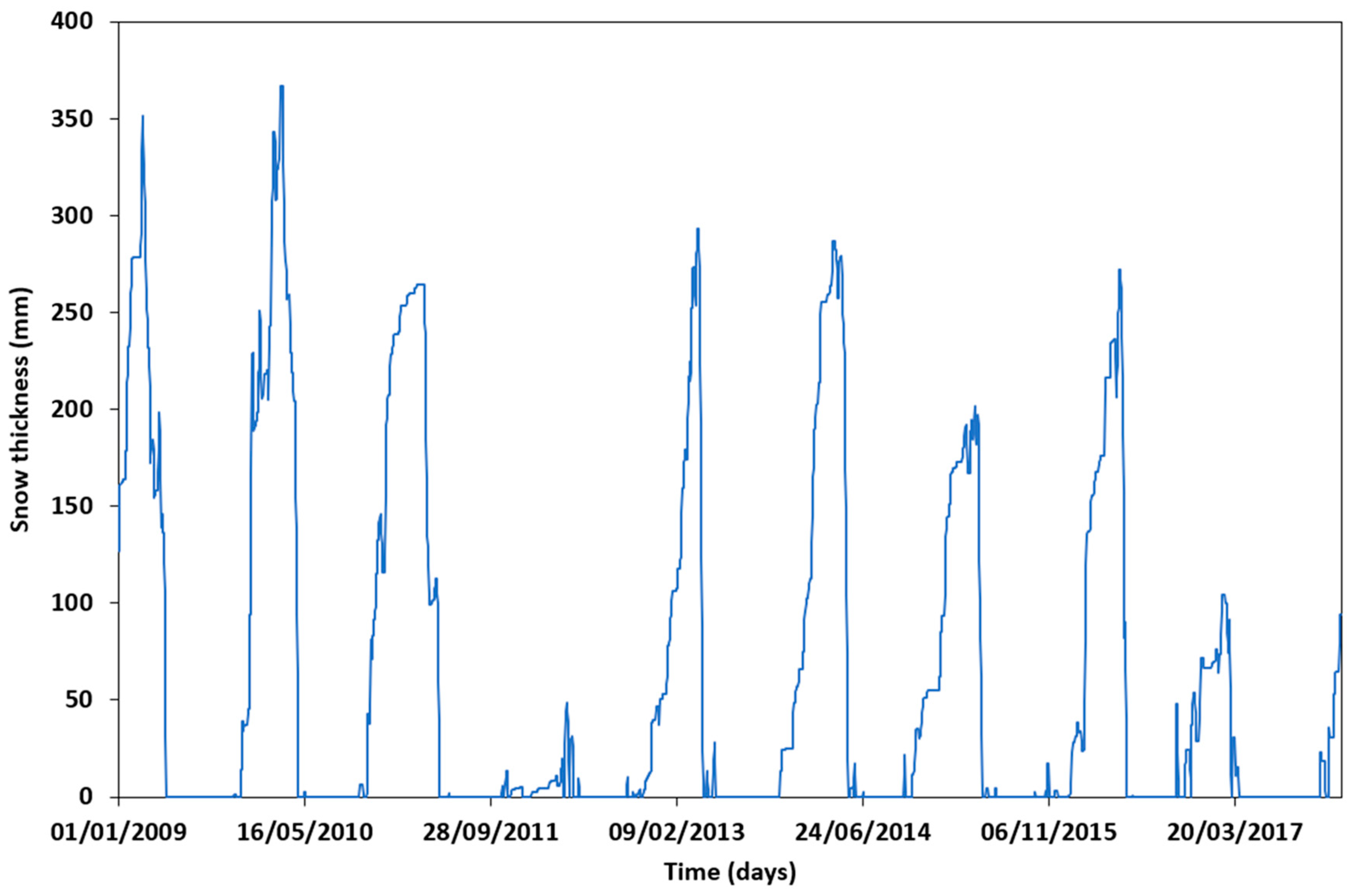
Figure 13 shows the experimental snow thickness data given in [
36,
37]. The thin line represents the point measurements of the changing thickness of snow over a four-year period at a point located in the Refugio de Poqueira (Sierra Nevada). The thick line represents the pixel measurements of snow from the dataset used in the work presented here and the previous simple model. The changing thickness results are similar but not identical because of the different supports (point and pixel) on which they are measured.
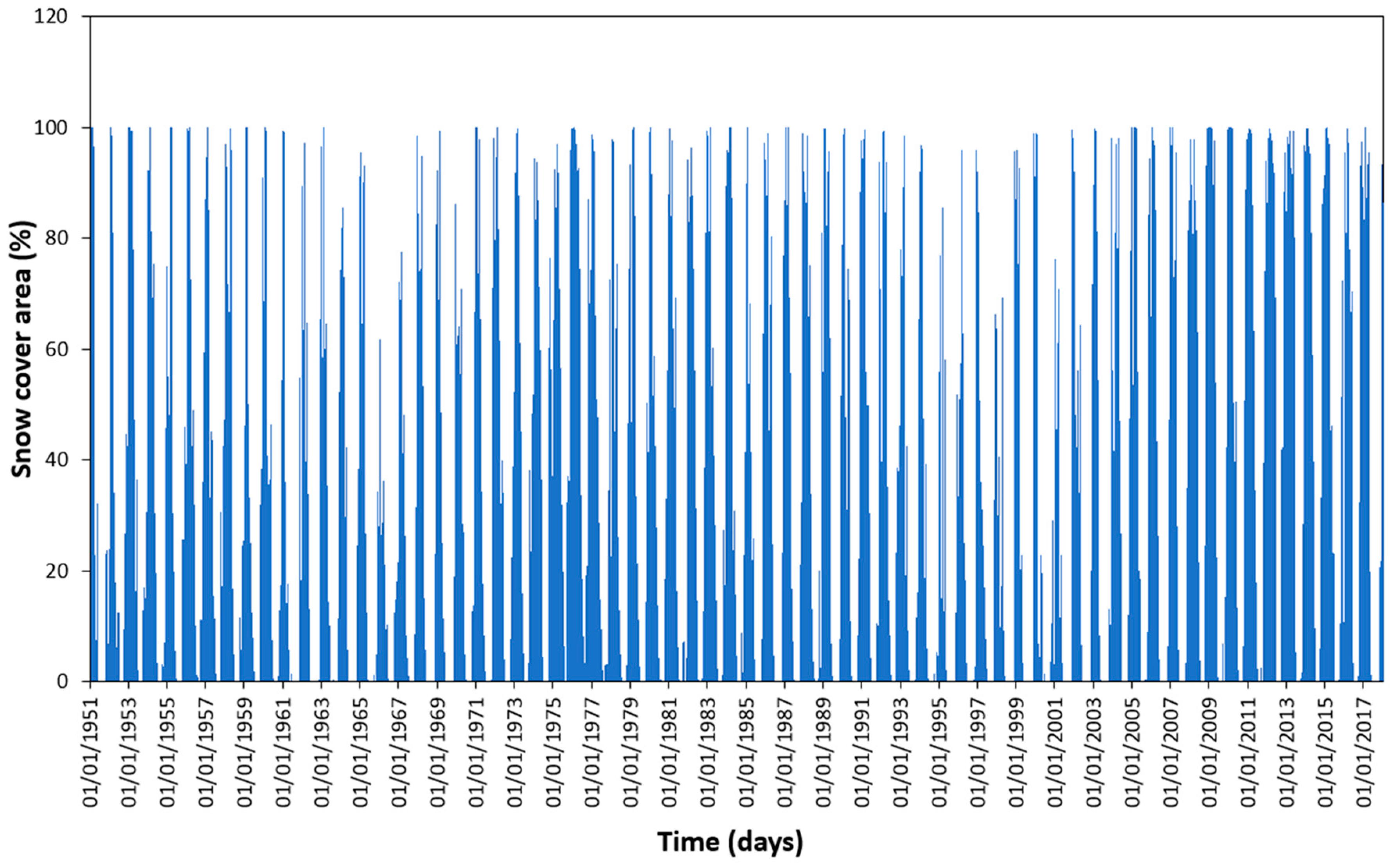
Figure 14 shows the changing area of snow cover in the Sierra Nevada mountain range over the 1951–2017 period. Days on which the entire mountain range was covered by snow are recorded as 100% snow cover. The detail of the snow-covered area is given in
Figure 15.
Figure 16 shows the thickness of snow in the cell that contains the ski resort town of Pradollano.
5. Discussion
Three important issues in the spatio-temporal dynamics of precipitation in the Sierra Nevada have been identified in this study: (1) the importance of orographic precipitation [
38] in understanding the spatial variability of mean annual precipitation; (2) the decreasing trend in the mean annual precipitation of 33 mm per decade; and (3) the NAO influence on mean annual precipitation. Other minor issues that have been revealed are (4) the persistence of seasonality over the almost seven decades studied and (5) the complex issue of the altitudinal precipitation gradient.
The precipitation patterns over the Sierra Nevada mountain range for the period of this study can be interpreted physically by considering the orographic effect and the main provenance of humid flows from the Atlantic and, to a lesser extent from the Mediterranean, that affect the Iberian Peninsula in general and the study area in particular. The authors of [
12] distinguished atmospheric patterns with a clear distinction between Atlantic and western Mediterranean disturbances that produce characteristic precipitation patterns over southern Spain. Most of the annual precipitation is drawn from the Atlantic Ocean and is mainly influenced by North Atlantic climatic processes [
39], such as the polar cyclone (Iceland Low), and hence the North Atlantic Oscillation (NAO) [
40]. Annual precipitation is sourced to a lesser extent from the Mediterranean and is mainly influenced by the Western Mediterranean Oscillation (WeMO) [
41]. Isotopic studies [
39] revealed two main sources of humidity that influence precipitation in the Mediterranean part of the Iberian Peninsula. Convective precipitation events from the Mediterranean are isotopically enriched and prevail during Summer (
Figure 10). In contrast, precipitation with lower isotopic values is transported along Atlantic storm tracks, which dominate during Winter [
42]. The authors of [
12] distinguished atmospheric patterns (synoptic types) with a clear distinction between Atlantic and western Mediterranean disturbances that produce characteristic precipitation patterns in Mediterranean Spain. In addition, from the synoptic types they obtained, The authors of [
12] summarised the main general scenarios that produce significant precipitation in Mediterranean Spain. The first scenario is a large-scale disturbance located to the west of the Iberian Peninsula and producing humid Atlantic flows that induce precipitation in western Andalucia. A second scenario is the passage of cold fronts over the Iberian Peninsula associated with higher latitude, low pressure systems that encourage precipitation in the mountainous areas of Andalucia. In a third scenario, relatively small lows at 500 hPa are found in the southern part of Spain, and the associated low-level flux over the Mediterranean from the east-southeast is warm and humid. This configuration leads to precipitation over the eastern flank of Spain [
12]. These three scenarios generated the three maxima in mean annual precipitation shown in
Figure 3A.
The observed decreasing trend, at a rate of 33 mm per decade, in mean annual precipitation in Sierra Nevada for the 1951–2017 period is consistent with findings by other authors. A general decreasing trend in precipitation in southern Spain from 1960 onwards was observed by [
43]. The authors of [
32,
44], among others, have also identified this decreasing trend of precipitation in southern Spain. Here, we have shown this decrease in the mean areal value of the high Sierra Nevada mountain range. The authors of [
45] studied the evolution over almost 100 years of the Azores high (the “centres of actions” for the weather in the Iberian Peninsula) and concluded that blocking anticyclones have become more prevalent over western Europe, which could explain the decrease in rainfall over the Iberian Peninsula in general and in the Sierra Nevada in particular.
There are clear correlations between the NAO index and the annual precipitation in the Sierra Nevada and between the NAO index and Autumn and Winter precipitation. This is because 73% of the annual precipitation occurs in Autumn and Winter. To a lesser extent, there is a correlation between the precipitation in Sierra Nevada and the WeMO index. The positive phase of the NAO reflects below-normal heights and pressures across the high latitudes of the North Atlantic and above-normal heights and pressures in the central North Atlantic [
46]. Hence, there is a northward shift of the axis of maximum moisture transport [
47], and thus, there is a decrease in precipitation over southern Europe in general (including Spain) and in the Sierra Nevada in particular.
Despite the variability of the total annual precipitation and its decreasing trend, there was variability, although there was no trend, in the seasonality for the observed 1951–2017 period. Here, seasonality has been defined as the percentage of annual precipitation comprising Winter precipitation. The conclusion is that, irrespective of the trend in annual precipitation, Winter precipitation will be the main seasonal precipitation contribution to the total annual precipitation.
Finally, there is the issue of the complex spatial gradient of mean annual precipitation with altitude. The altitudinal gradient between locations A and B can be defined as:
where
is the mean annual precipitation at location
A and
is the altitude of location
A. Given that the order of the locations is
, a positive gradient means that precipitation increases with altitude. It is clear from
Figure 3B that the altitudinal gradient of precipitation for Sierra Nevada will be complex. Because of the orographic effects shown in
Figure 3, in the best case (considering the windward side of the Sierra Nevada mountains), there will be an altitudinal gradient in the mean annual precipitation of 15 mm/100 m. There will be a gradient of 10 mm/100 m in the mean annual precipitation for the best location on the lee side of the Sierra Nevada mountains. However, in general, the altitudinal gradients will be smaller if any two arbitrary locations are considered. These altitudinal gradients in precipitation are significantly different to some of the values reported in the literature for the Sierra Nevada mountain range, e.g., 170 mm/100 m reported by [
48], among others.
With respect to the spatio-temporal dynamics of temperature in the Sierra Nevada, there are several points that have been identified in this study:
- (1)
The spatial distribution of temperature is highly correlated with altitude, with correlation coefficients of 0.85 and 0.9 for minimum and maximum temperature, respectively.
- (2)
The annual temperature trend has a negative slope but, as it is not statistically significant, the annual temperature in the Sierra Nevada cannot be considered to be decreasing, even in terms of the minimum, maximum, or mean temperatures.
- (3)
The spatial variability of the trend in annual temperatures is complex. There are areas that show an increasing trend while others show a decreasing trend and others are undefined, as the trend is not statistically significant.
- (4)
By using a simple degree-day model, it is possible to evaluate the evolution of the Sierra Nevada snowpack by assessing a large number of spatial and temporal statistics. For example, the transient seasonal snowline could be evaluated.


