3.2.1. Survey Data as an Input
In order to create a model based on observed daily mobility, one of the most thorough dataset available in France is the "Enquête Ménages-Déplacement", or "EMD" (household travel survey). This standardized survey is focused on the daily mobility in large urban districts.
The data production draws upon questionnaires given to randomly-selected households inside specific representative zones of the urban area, between the end of November 2009 and beginning of April 2010, excluding holidays and weekends. The collected data are focused on the day preceding the survey for each individual, and cover a 24 h period, in which every journey must be as detailed as possible in space and time.
The 2010 EMD survey used in this work collected 7600 households from Grenoble’s urban area in 97 districts, which means around 16,000 people aged 5 years and over.
We elaborated a typology of the population according to their socio-economic and demographic characteristics. The statistical aggregation method also keeps the groups different enough in their characteristics and numbers (
Table 1).
Table 1.
Typology of population according to their socio-economic, demographic characteristics and daily activities.
Table 1.
Typology of population according to their socio-economic, demographic characteristics and daily activities.
| Category | Headcount |
|---|
| 1: Active people | 3914 |
| 2: Single mothers/Part-time workers | 1313 |
| 3: Unemployed | 577 |
| 4: Active and unemployed 40–64 years old people | 2706 |
| 5: Students | 1283 |
| 6: Retired people | 2131 |
| 7: Young people (going to school) | 2897 |
3.2.2. Data Process and Validation of the Results
Based on these categories, a synthetic population could be generated following four important steps: (i) definition of attributes that will be assigned to agents; (ii) generation of agents under constraints of attributes using GenStar (Gen*) prototype [
19]; (iii) validation of the population obtained; (iv) spatial allocation of agents created.
The following table (
Table 2) illustrates the chosen attributes to be assigned.
Table 2.
Attributes assigned to the synthetic population.
Table 2.
Attributes assigned to the synthetic population.
| Attribute | Dependencies | Levels |
|---|
| Category | age | [1,2,3,4,5,6,7] |
| Age | category | 5:17, 18:24, 25:34, 35:49, 50:64, 65:100 |
| Gender | category | man, woman |
| Area | category | One of the 97 area |
| Main Activity | category | Work, Study, Shopping, etc. (8 possibilities) |
| Vehicle type | age, area | No vehicle, authorized vehicle (registred after 2001), un authorized vehicle (registred before 2001) |
The synthetic population is then generated with the Gen* algorithm [
19], using a learning sample of the initial survey data. The frequency of each desired attribute is extracted from the survey, with its dependency to an other attribute. The
Table 3 below gives an example of the frequency of people from the survey who are male (Gender = 1) depending on their category (from 0 to 2 in the example). Gen* will use such inputs to generate a conditional probability law for every attributes.
Therefore, empirical probability laws for every attribute and its dependencies (conditional probabilities) can be generated, as the basis of a statistically coherent synthetic population.
Then, the validation procedure per se follows three steps.
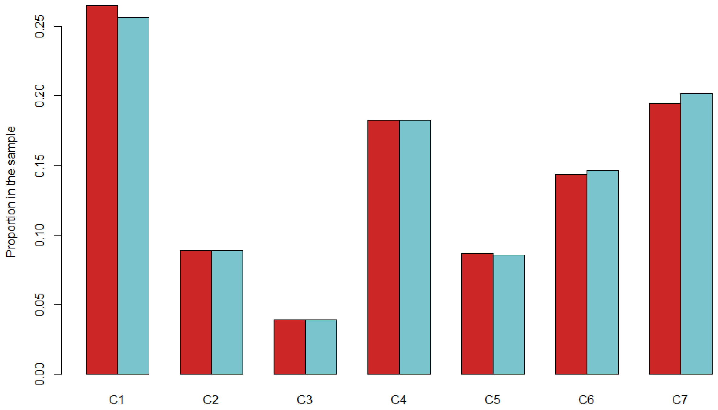
Firstly, we use 10 random subsets—called learning sets—extracted from a percentage of the individuals of the EMD survey, in order to generate a synthetic population with Gen*. Then we compare these subsets with the rest of the population, which is the validation set (
Figure 4).
Table 3.
Example of conditional probability law for male agents.
Table 3.
Example of conditional probability law for male agents.
| Category | Gender | Frequency |
|---|
| 0 | 1 | 1992 |
| 1 | 1 | 183 |
| 2 | 1 | 273 |
Figure 4.
Difference in categories’ proportions between 90% and 10% learning sets.
Figure 4.
Difference in categories’ proportions between 90% and 10% learning sets.
Secondly, we average the attributes of the generated population and the subsets. We compare them.
Thirdly, we compute relative errors between the learning subset and the synthetic population (
Table 4).
Table 4.
Relative errors for the main attributes.
Table 4.
Relative errors for the main attributes.
| Attribute | Value | Relative Error |
|---|
| Category | 0 | 0.007 |
| 1 | 0.012 |
| 2 | 0.008 |
| 3 | 0.006 |
| 4 | 0.016 |
| 5 | 0.002 |
| 6 | 0.001 |
| Gender | Man | 0.001 |
| Woman | 0.001 |
| Age groups | [5;17] | 0.001 |
| [18;24] | 0.011 |
| [25;34] | 0.001 |
| [35;49] | 0.011 |
| [50;64] | 0.006 |
| [65+] | 0.002 |
| Area | [100;199] | 0.002 |
| [200;299] | 0.011 |
| [300;399] | 0.004 |
| [400;499] | 0.008 |
| [500;599] | 0.005 |
| [600;699] | 0.019 |
| [700;799] | 0.036 |
| [800;899] | 0.013 |
| [900;999] | 0.006 |
Even if the learning subset is around 50%, the relative error is globally under 5%, and the methodology used does not produce any incoherent combination of attributes, as soon as the frequency is equal to 0 in the input file.
Other attributes that are not shown here are aggregated values from the global survey, and cannot be specific to a subset of the population. They are nonetheless well distributed as well.
3.2.3. Localization of Agents
Once generated, agents are randomly allocated to a living place—under constraints of capacity—within the zone they belong to. Then, a working (or their other main activity) place is assigned as well, but without restriction on the zone.
To simplify the model, there is no affectation of agents to households yet. This means that agents are randomly located in buildings together. The diversity of people at the building’s scale is expected to offset the lack of details at the households scale.
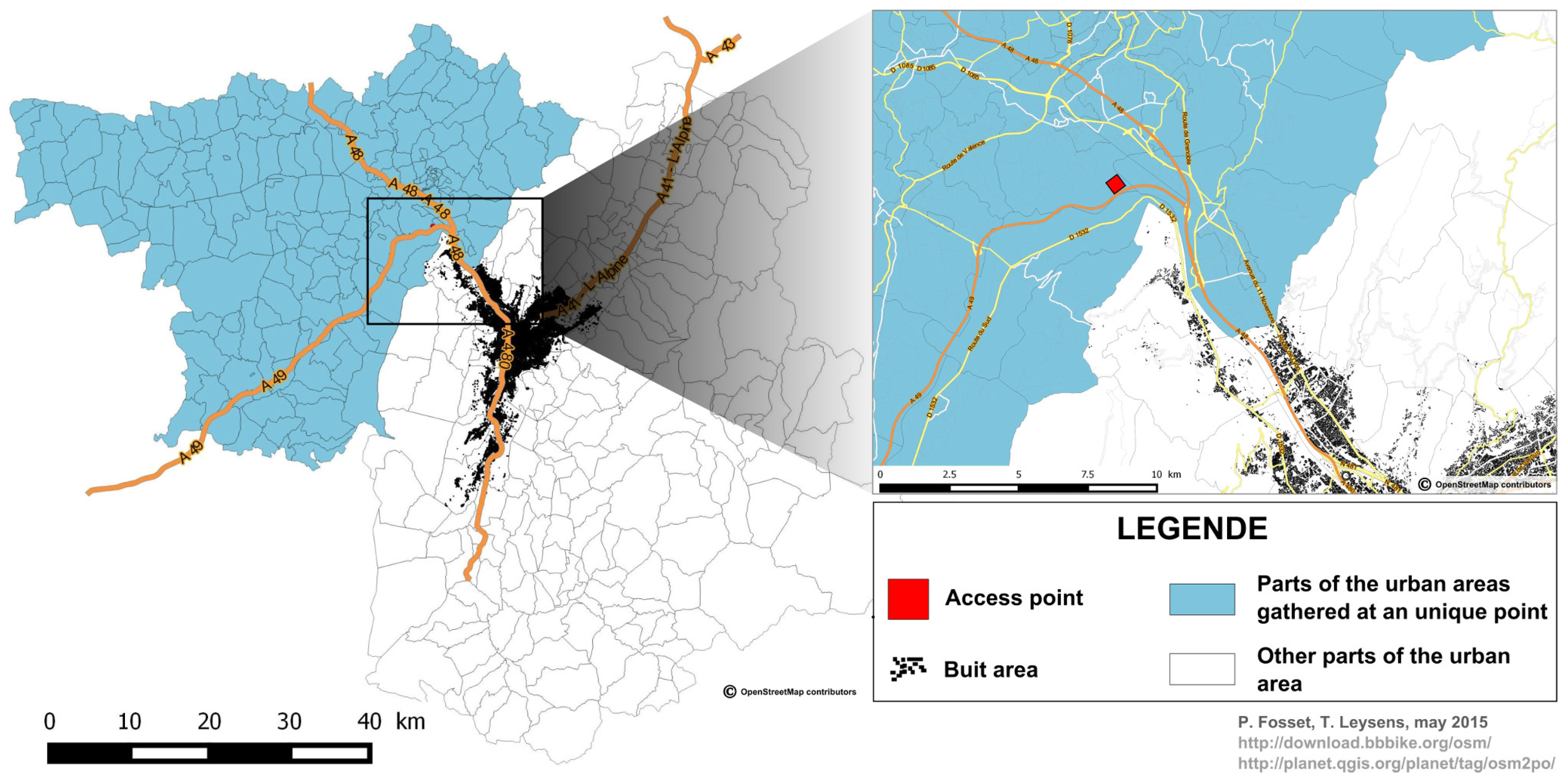
Moreover, as survey data cover a much larger area (urban area of Grenoble) than our limited case study does, we made sure to take into account populations coming from external areas, allocating them as agents to a limited number of “access points” localised on the main road axis of the urban system (
Figure 5).
Figure 5.
Concentrating external areas in one point.
Figure 5.
Concentrating external areas in one point.
3.2.4. Generation of Agent’s Schedule
Once created, each agent picks-up a schedule in a predefined library of schedules (
Table 5).
The predefined library of schedule, is derived from the full sets of combinations revealed by the EMD survey. A Python program, has been developed in order to create a set of around 5000 possible combinations of activities, according to the EMD survey.
At first, the logical combinations of all activities are generated, under the following list of constraints: existence of minimum (1) and a maximum (3) number of activities in a day; necessity for schedules to begin and end at “Home”; absence of redundancy for “Home”. These conditions are based on the analysis of the survey, revealing that the part of the population concerned by a schedule with more than three daily activities is not significant. Indeed, in every category except from the single women and partial time workers, it represents less than 2% of the combinations.
All the remaining logical combinations are sorted by main activity in a csv file, from which the schedules will be chosen and scheduled.
Several steps are implied at this level, to schedule the previously-selected schedules.
Table 5.
Schedule library extract (person #0, Main activity “Work”, time in second).
Table 5.
Schedule library extract (person #0, Main activity “Work”, time in second).
| ID_Pers | ID_Schedule | ID_ACT | ACTIVITY | DATE_BEGINNING | DATE_ENDING |
|---|
| 0 | 0 | 0 | Home | 0 | 49,440 |
| 0 | 0 | 1 | Work | 49,500 | 62,233 |
| 0 | 0 | 2 | Sport | 62,533 | 65,206 |
| 0 | 0 | 3 | Work | 65,326 | 78,059 |
| 0 | 0 | 4 | Home | 78,119 | 86,400 |
| 0 | 0 | 0 | Home | 0 | 29,091 |
| 0 | 0 | 1 | Study | 29,151 | 33,701 |
| 0 | 0 | 2 | Work | 33,881 | 60,751 |
| 0 | 0 | 3 | Study | 60,931 | 74,579 |
| 0 | 0 | 4 | Home | 74,369 | 86,400 |
First, we assign a main activity to each agent, according to his category and the occurrence of each activity in the schedules (provided that it exceeds 10%) from the survey.
Second, we assign the living place and main activity place to each agent, then using the library of schedules, we propose a limited number of schedules to each agent, in order to keep the choice at a realistic scale [
20].
This choice is limited by the main activity that must appear in the list of activity of the schedule. We propose 10 schedules that are randomly chosen in the library.
Agents will choose a schedule in this set using utility functions (see
Section 3.2.2). The parameters taken into account are: the proposed activities, the matching between these activities and agent’s category but also the time needed to reach and achieve these activities (see
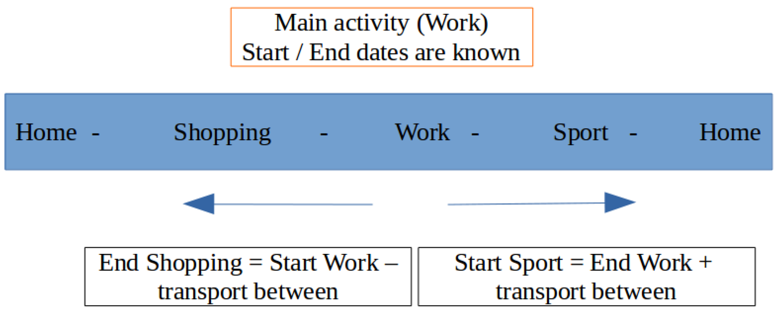
Section 3.2.5). Based on this, we construct a time sorted schedule with, for each activity, a beginning and an ending date (
Figure 6).
Figure 6.
Schedule creation.
Figure 6.
Schedule creation.
We first determine the duration of the main activity, based on the mean value depending on the category. Then, we determine a time interval during the day, based on the building’s schedule concerned by the main activity and on its duration. From this duration, we randomly assign a beginning date within the interval.
From this main activity starting date, we calculate the schedules for the activities that come after and before, by subtracting the mean transportation time (always depending on categories) between them, and taking the mean time of each one as a duration. We do so, until we reach the first and last activities of the schedule.
Transportation durations and main activity durations are based on average durations from the EMD survey, and are specific to each category. The durations follow a normal distribution.
For other activities, including the time spent at home, the mean time is also used, but the proportion of the day each activity covers is calculated in order to make the durations are realistic.
3.2.5. Utility Function and Decision Process
Each agent faces distinct schedules that are theoretically feasible and mutually exclusive (representative activity patterns). Decision process is then formalised with discrete choice models that are appropriate to bring out individuals’ preferences under the assumption of rational behaviour. The goal of these models is to understand, in a somewhat causal approach, the factors that lead to individual choices in various contexts. These factors are introduced in a utility function that is supposed to “explain” the choices made and that summarises agents’ preferences.
The most widely used discrete choice model is the logit model decomposed into representative and unobserved utility [
21]. In a choice set, each alternative could provide a certain level of utility for the agent. The utility that decision maker n obtains from alternative i is determined by its attributes k (representative utility). Unobserved factors related to strictly individual preferences can be added as a random term Euro (unobserved utility). However, in the logit model, this random term is assumed to be identically distributed among individuals, which is relatively consistent with the definition of our seven homogeneous groups (
Table 1). This assumption is restrictive but provides a convenient and easily interpretable expression for choice probabilities.
Although more complicated expressions are possible, representative utility functions are usually formulated as a linear additive function of attributes chosen by the modeller. The utility
is defined as Equation (
1).
where
is a vector of coefficients allocated to the potential explanatory variables
.
The data source for the calculation of the discrete choice parameters is the French “Enquête Mênages Dêplacements”. Variables tested in the model are duration and travel time associated to various out-of-home activities. The utility of a schedule (or an activity pattern) is comprised of the utilities of time spent in each out-of-home activities (positive coefficient expected) and travel time from the location of an activity to another one (negative coefficient expected).
Under the principle of utility maximization, the decision maker is expected to choose the alternative that provides him the largest utility among a reduced choice set. However, the agent’s choices are not strictly deterministic and the behavioral process is based on probabilities estimation. We can define the choice probability of each activity pattern evaluated by the agent. The probability
that an agent chooses an alternative is simply a function of its representative utility
into the set of all evaluated activity programs
. This probability is expressed as Equation (
2).
Although, the probabilities of choice are distributed in a disaggregate way, according to the utilities calculated for each individual [
22], the outcomes of the logit model provides an approximation of groups preferences that lead to activity program choice.
The calibration of the model is based on a selection of significant variables for which parameters
are determined with the maximum likelihood method [
23]. The variables are considered statistically significant if their p value remains lower than 0.05. Only significant variables are shown in the following outcomes (
Table 6, with the following symbols for the corresponding
p values : *
p < 0.05, **
p < 0.01, ***
p < 0.001).
Results show a classical strategy of maximization of several activity-times with a travel-time minimization. Travel time is not as frequently significant as expected but note that time spent in transport reduces the amount of time available for time activity.
Table 6.
Utility functions for different activities and population categories.
Table 6.
Utility functions for different activities and population categories.
| | Active People | Single Mothers/Part-Time Workers | Unemployed | Active and Unemployed 50–64 Years Old People | Students | Retired People | Young People (Going to School) |
|---|
| Working time | 0.584*** | 0.358*** | | 0.312*** | 0.152*** | | |
| Travel time to work | | | | | | | |
| Study time | | | | | 0.118*** | | 0.135*** |
| Travel time to place of study | | | | | −0.124*** | | −0.166*** |
| Purshasing time | 1.36** | | 5.12*** | 2.18*** | 0.236*** | 2.26** | |
| Travel time to purshase | −0.242*** | | | −0.257*** | −0.286*** | −0.127*** | |
| Health time | | | | 0.811*** | | 0.5*** | |
| Travel time to health facilities | | | | −0.167*** | | −0.268*** | |
| Administrative procedures time | | | 0.307*** | | | | |
| Travel time to administrative procedures | | | −0.303*** | | | | |
| Leisure time | 1.77*** | 2.0*** | 3.16*** | 6.18*** | 0.313*** | 2.13*** | 0.39*** |
| Travel time to leisure activity | | | | | | | |
| Accompanying time | 2.58*** | 4.0*** | | 4.48*** | | | 0.25* |
| Lunch time | | | | −0.191*** | 0.231*** | | |
| Travel time to lunch | | | | −0.078 | −0.087 | | |
The outcomes of the modelling that is the final form of the utility function synthesizes groups’ preferences that will be used in the simulation. Thus, utility functions are used by agents, according to their group assignment, to choose an activity and travel time schedule in a choice set. From this point, agents expect a certain level of utility from the chosen alternative and compare it with the utility really obtained in the simulation (satisfaction measure).
These functions can capture tradeoff or compromise effects between time spent on several specific activities and travel time to reach activities localizations. That is the same level of utility can be reached with different activity programs in term of activities chosen, location and mobility behaviour. This ensures a wide range of agents behaviour.
The level of satisfaction is calculated from the utility function. If the satisfaction obtained into the simulation is below the expected one from a certain threshold level, agents can change their route, modal choice or the location of their activities before choosing a new schedule available in the library. The real utility of this new schedule should be comprised between its expected utility and the expected utility of the previous schedule chosen.


 ,
, 


