1. Introduction
The US housing market crisis that began in August 2007 has led to a vast literature that has offered several, sometimes contradictory, causes for the crisis. This paper uses a system dynamics model of household finance to understand how some of the main hypothesized causes, working through household and institutional level decision-making based on information availability and incentives, influenced the outcomes in the market for homes. While there are a large number of explanations available, a majority of them fall into just a few broad categories. In particular four of the most comprehensive categories are the shortcomings of the institution of financial regulation, the availability of “cheap” money for households, the Federal Reserve’s expansionary monetary policy and bankruptcy reform.
The paper contributes to the literature by using a formal model to test whether the reasons cited by the extant literature could indeed be the causes of the housing crisis. Our test consists of simulating and checking against observed data. This question is difficult to address using standard empirical methods, such as regression analysis and event studies. Even if all the relevant data were available, it is unlikely to separate the effect of each cause. Our formal model allows us to achieve this. We replicate the assumptions made in the literature and then test each cause. Our results show whether the causes cited are indeed able to replicate the crisis. The added benefit of this approach lies in offering a formal platform, which other researchers may use to test alternate hypothesized causes and assumptions.
The institution of financial regulation has been blamed for a number of problems that precipitated the crisis. For example, it has been blamed for not evolving quickly enough to devise appropriate policies to keep pace with financial innovation [
1] and for assigning inordinate importance to credit rating agencies in determining the success of issuing of securities [
2]. The latter is believed to have led to credit rating agencies giving more importance to their input into the securities issuing process rather than informing investors about the risk of their investments. Ultimately financial regulation is believed to have led to overly easy credit availability to households as well as businesses.
Another category of explanations is “cheap” money, which is hypothesized to have been available to households due to rising savings abroad, rising equity in homes, and the government’s mandate to increase home ownership. Rising savings abroad meant cheaper loans in the US as foreigners invested in low yield US assets [
3].
Among other sources of cheap money during this period was the accelerated growth of home equity. Home prices rose about six percent annually in 1998 and 1999, and 10 percent from 2000 to 2003 followed by the most rapid gains of about 16 percent in 2004 and 2005 [
4]. The rising value of homes in the US provided cheap money to households particularly due to the sophistication of financial markets which made it possible for households to easily access this value through cash-out refinancing and home equity lines of credit. A final source of cheap money for households was the US government’s mandate to extend homeownership.
The third category of hypothesized causes for the crisis is the conduct of US monetary policy during the first half of the decade of the 2000s. The stock market collapse following the dot-com bust, led to a moderate recession in the US. This was followed by the terrorist attack in New York on 11 September 2001 that further diminished investor confidence. These developments led to an expansionary monetary policy. Expansionary monetary policy persisted through most of the first half of the last decade fueled by a series of corporate scandals, slow job creation and the perceived threat of deflation [
1]. Expansionary monetary policy has been put forth as a cause contributing to the home price bubble in the US. However, some of the evidence supporting this theory is contradictory.
In addition, bankruptcy reform reduced protection so that homeowners were forced to service other debt instead of having the option to concentrate on their home mortgages. This could have fueled an increase in mortgage defaults [
5].
In this paper we attempt to assess the relative importance of the main causes hypothesized in the extant literature as explanations for the financial crisis in the US. We construct a system dynamics model of the personal saving and investment decisions of households and experiment with it to assess the impact of each cause. This framework allows us to understand the mechanism through which each hypothesized cause might influence the market for homes and the household finances in the economy. We study whether the hypothesized causes could potentially lead to crisis situations. We also overlay each cause on the others to mimic the actual chronological order in which the real world situation unfolded. This helps to demonstrate how multiple causes, working together, might impact the market for homes and household finances in the economy; in particular, whether they might magnify or dampen one another’s effect when implemented simultaneously in our model.
In chronological order, the major categories of causes that are hypothesized to have led to the crisis occurred in the following: First, the earliest cause can be traced back to 1975 when the credit rating agencies were elevated in status. This along with failure to keep pace with financial innovation is hypothesized to have led to overly easy credit availability to households and firms. This process is subsumed in our first experiment. Second, the availability of cheap money via the government’s encouragement of home ownership dates back to the Community Reinvestment Act in 1977. This along with cheap money from developing country savings exported to the US is hypothesized to have led households to overinvest in homes. This process is added to the system in our second experiment. Third, the Federal Reserve lowered interest rates starting 2001 and kept them low well into 2004, which enters the system in our third experiment. Finally the bankruptcy reforms of 2005 have been hypothesized to have increased the default rate on home mortgages, which we add to the system in our fourth experiment.
Our findings indicate that each tested cause contributes to the crisis in a unique way. The lax financial regulations contribute to both the increase as well as eventual decline of housing prices. Cheap money influx contributes to the increase in home prices, however it actually cushions the fall in prices. In contrast, the lowering of the interest rate by the Federal Reserve, while contributing to the fall in prices, actually dampens the initial price increase. Bankruptcy reform contributes to the fall in prices.
Interestingly our experiment representing the Federal Reserve’s lowering of interest rate has an impact on home prices predominantly through lowering households’ incentive to save. This results in a smaller rise in home prices due to households’ reduced savings. However, when the home price bubble bursts, lower interest rates make the crisis worse because households are ill-equipped to handle the downturn due to low accumulated savings. This somewhat vindicates the Federal Reserve’s stance that lower interest rates did not feed the bubble. At the same time it draws attention to household savings as the route through which this policy might have played a role in the crisis.
Finally we confront our assumptions and our results with actual data surrounding the US housing crash of 2007. This helps to justify our assumptions and to test which of the hypothesized causes of the crisis are able to replicate the real world outcome. Our assumptions are broadly justified by the US data and our simulation results are supported strongly as well.
The rest of the paper is organized as follows.
Section 2 presents some controversies in the literature that have a direct bearing on this paper.
Section 3 presents our model and confronts assumptions made with US data.
Section 4 presents our experiments and findings and compares them with US data.
Section 5 concludes.
2. Literature Review: Controversies
The introduction has presented much of the relevant literature. We concentrate in this section on two of the four causes we investigate in this paper. Specifically, we delve into the controversies that surround monetary policy and availability of cheap money as causes of the housing crisis. While there is broad consensus on regulatory failures and bankruptcy reform as causes of the crisis, the role of cheap money and monetary policy remain less clear-cut.
We tackle the monetary policy controversy first. Bernanke [
1] provides a defense of the monetary stance during the years when the housing market was booming based on the underlying weak economy that needed monetary stimulus. Furthermore, home prices simultaneously rose in a number of countries. Cross-country comparison indicates that there is a strong positive relationship between current account deficits and home price appreciation rather than monetary policy and home price appreciation. In addition, expansionary monetary policy tends to improve the current account balance through a weaker currency that spurs exports and reduces imports. In addition, the historical relationship between monetary policy and home prices indicate that monetary policy could have been responsible for only a small portion of the increase in home prices seen in the early 2000s [
6,
7,
8,
9]. One possible reason for monetary policy to have influenced home prices more than historical relationships warrant could be financial innovation [
9]. For example adjustable rate mortgages made short-term interest low enough that it brought previously unaffordable homes within reach of some households.
The controversy surrounding cheap money deals with its source and importance as a cause of crisis. An important source of this cheap money is hypothesized to be excess savings from developing countries. This saving was exported predominantly to the US due to a conscious policy of accumulating war chests of foreign exchange reserves Bernanke [
3]. These reserves were meant to protect economies against the perceived risk of crisis due to uncertain international capital markets. This was even more so given the number of financial crises in developing countries from Asia to Latin America over the course of the 1990s and early 2000s. The US was the choice destination for these savings because of the special status of the US dollar as international reserve currency.
On the other side of this debate are models that demonstrate that the asset price bubbles in equity and residential real estate, and not cheap money, led US consumers to overspend. An example is Liabson and Mollerstrom [
10] who contends that this is more likely representative of reality since capital imports in the US were consumed and not invested which is counter to what would be expected if foreign savings were responsible for the cheap capital in the US. Bernanke [
3] provides the counter argument that while capital exports from developing countries were attracted by high investment returns up to the dot com bust in 2000, savings continued to follow into the US later simply as a precautionary measure to build war chests of foreign exchange reserves, as outlined above.
Another source of cheap money were Government Sponsored Entities (GSEs): Federal National Mortgage Association (Fannie Mae, CT, USA) and Federal Home Loan Mortgage Corporation (Freddie Mac, VA, USA). These entities raised money cheaply since they are implicitly backed by the government. In this context their primary function is to create a secondary market for mortgages: they purchase mortgages from banks and other primary mortgage lenders and hold them or package them into Mortgage Backed Securities (MBS) guaranteeing timely payment of interest and principle and sell these to investors. There were two policies that expanded mortgage markets and encouraged GSEs to accept lower quality mortgages and thus encouraged upstream primary mortgage lenders to lower their lending standards as well [
2]. These were the expansion of the affordable housing mission of the GSEs and the Community Reinvestment Act (CRA).
3. The Model
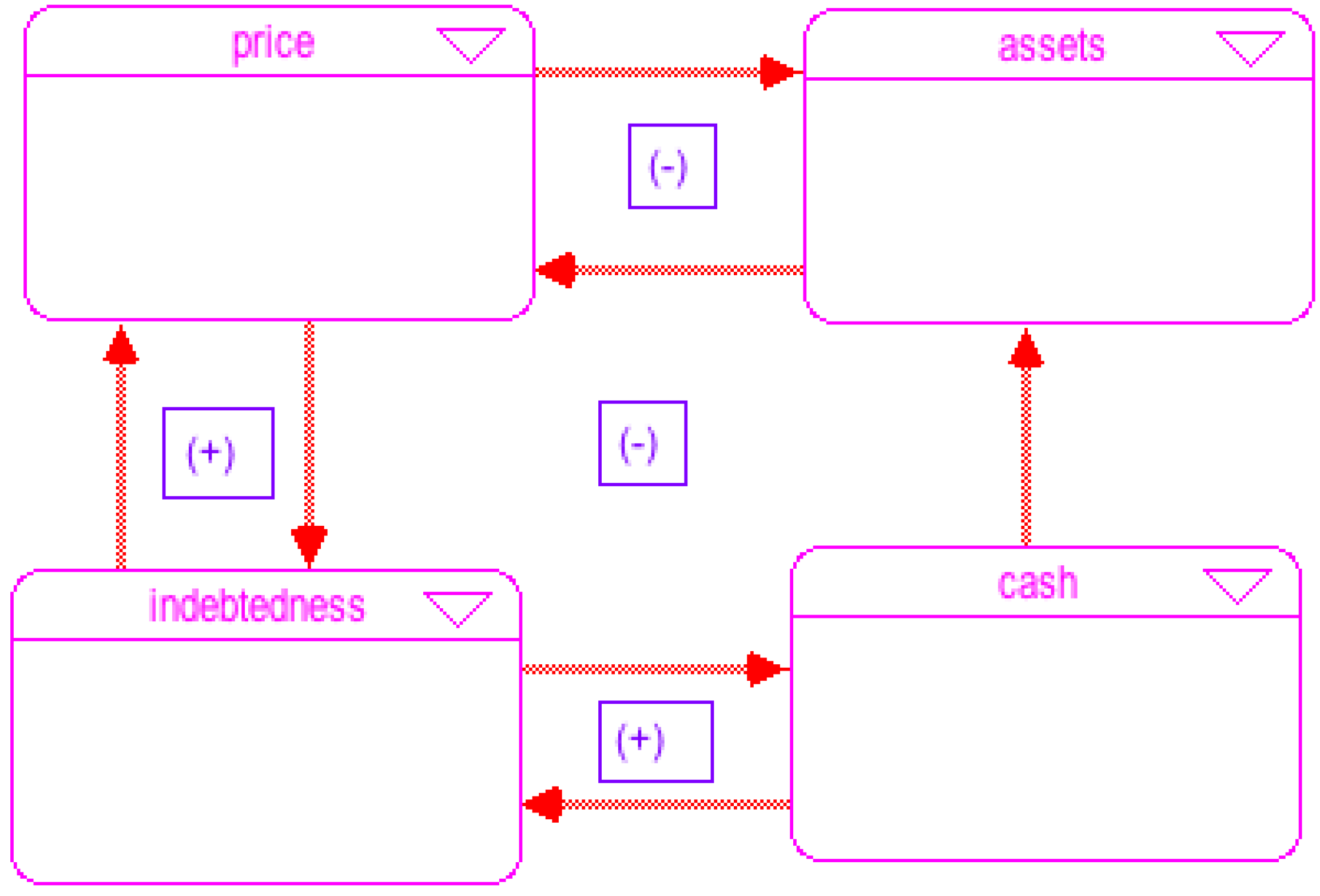
In this section we present the model of a system that describes the financial decisions of households. It takes into account the information available at the decision point, cognitive processes through which this information is processed and incentives built into the structure of the economy that together determine the financial policy pursued by households. An aggregate view of the model appears in
Figure 1, which shows the relationships between the sections into which the model is divided.
Figure 1.
Aggregate relationships in the model.
Figure 1.
Aggregate relationships in the model.
The model has four interrelated sections: real estate volume, real estate price, household debt and available cash for households.
Figure 1 represents the two-way relationships among these four sections and the fact that they are simultaneously determined in our model. The only assets in the model are homes. Real estate volume and real estate price are related directly, as well as through changes in household debt and available cash. Household debt and cash available for investment can grow together because rise in home prices lead to gains in equity for home owning households, allowing them to borrow even more. Finally, available cash reduces indebtedness through debt service.
A detailed view of each section of the model is presented in
Figure 2,
Figure 3,
Figure 4 and
Figure 5 and related equations are presented alongside in the text. These figures are representations of the model programmed in
ithink, which is the simulation software used to implement our experiments. These diagrams are helpful in visualizing the model succinctly before we introduce the model equations. Following the standard system dynamics notation, stocks are rectangles, flows are valve symbols, and parameters and intermediate computations are circles. Arrows indicate mathematical relationships between variables. To read more about the system dynamics methodology, please refer to [
11], a comprehensive one-volume reference on system dynamics.
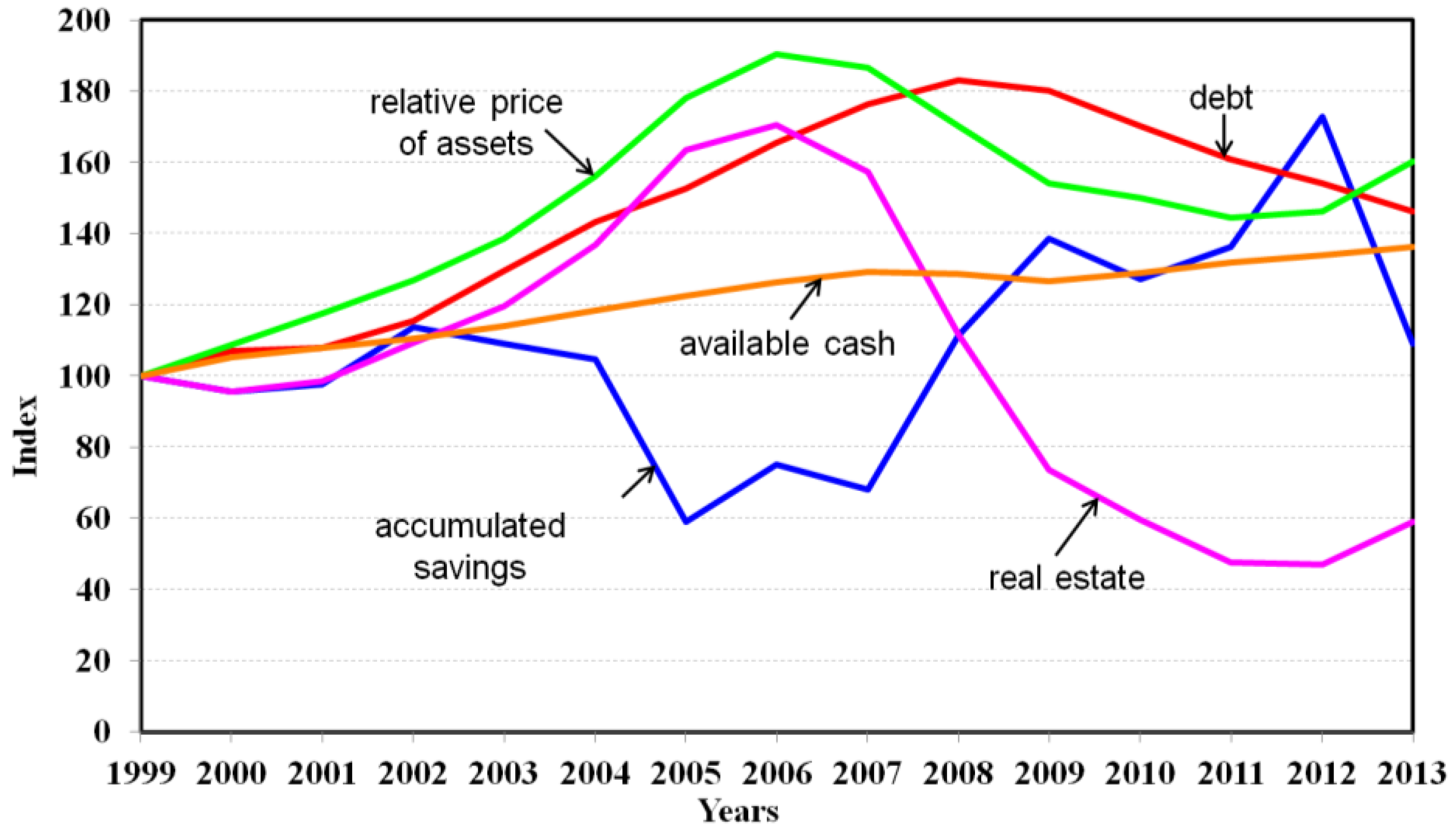
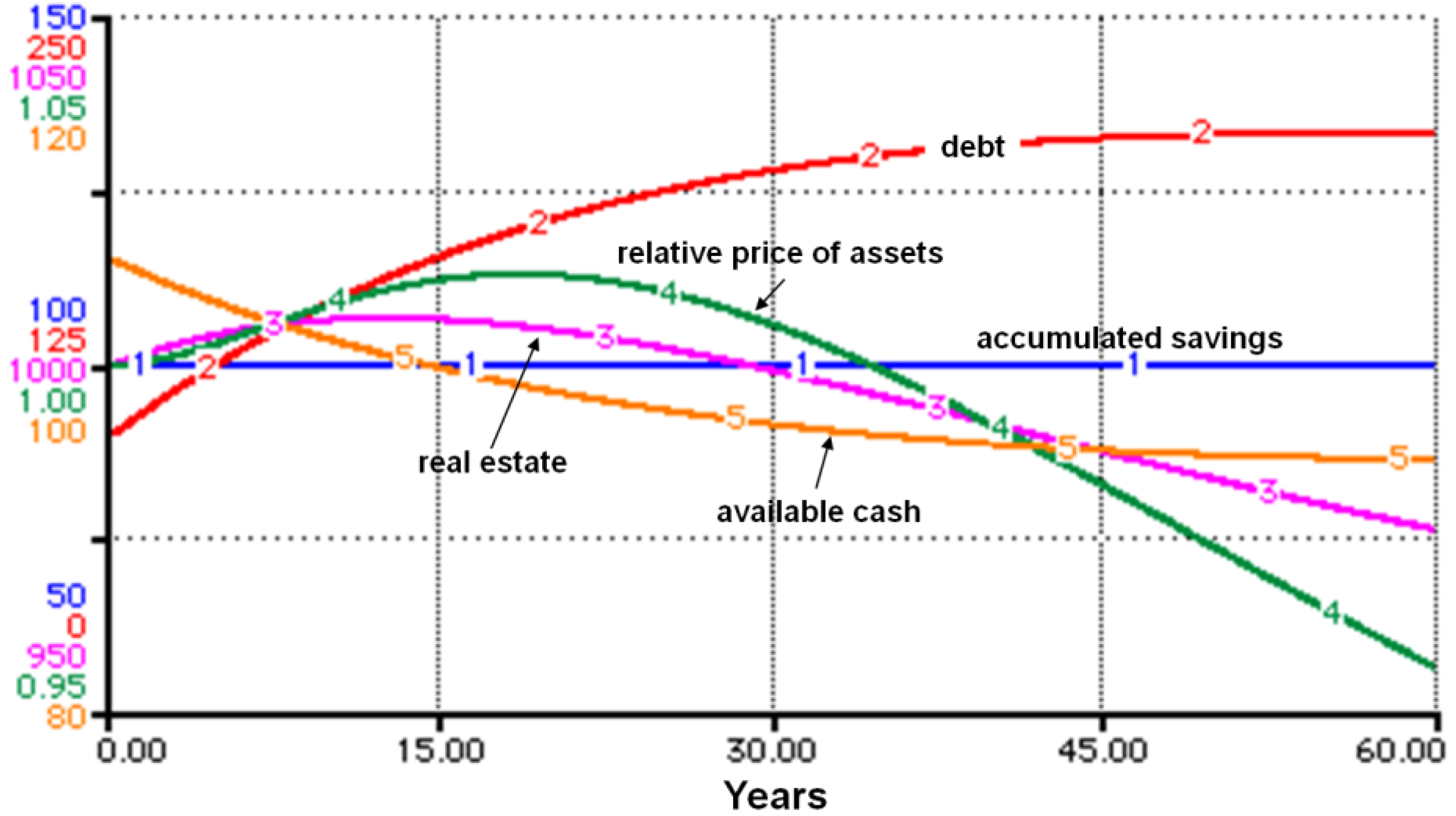
We present actual data relating to each of the outcomes of our model. Real estate volume is proxied in actual data by the US Census Bureau’s new residential sales, real estate price by the Case-Shiller index, household savings by the personal savings rate of the Fed, available cash by the BEA personal expenditure data and household debt by Fed data. Definitions, sources and calculations of the US data are in
Table 1 and the data is presented in
Figure 6 (the graph presents the data in index form, the raw data is available from the authors upon request).
Table 1.
Real data source and description.
Table 1.
Real data source and description.
| Variables | Source | Data Manipulations |
|---|
| Real Estate Volume | New Residiential Sales, US Census Bureau, available at [12] | None |
| Real Estate Prices | Case-Shiller Home Price Index, available at [13] | Monthly House Price Index were averaged in order to obtain annual index. |
| Debt | Consumer Credit Panel, Federal Reserve Bank of New York, available at [14] | Annual data calculated by averaging quarterly data. Nominal dollars converted to real dollars by deflating by the CPI. |
| Available Cash | National Income and Product Account Tables, Bureau of Economic Analysis, available at [15] | None |
| Accumulated Savings | Personal Saving Rate, Federal Reserve St. Louis, available at [16] | None |
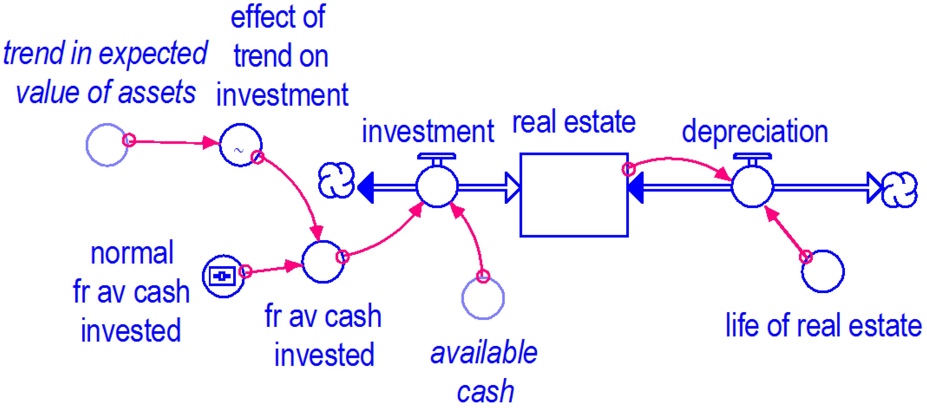
3.1. Real Estate Volume
Figure 2 describes the asset market,
i.e., the market for homes. In
Figure 2, real estate is a stock variable, depreciation and investment are flows. The normal fraction of available cash that is invested is an example of a parameter. The figure depicts how real estate volume is determined by the interaction of depreciation and investment. Investment is determined by household decisions, which are influenced by the trends in the price of real estate. Every home bought is assumed to be newly built. The volume of real estate, H, in the asset market adjusts over time according to the following equations:
where
I is investment,
Dep is depreciation,
C is available cash for households,
is the average fraction of available cash that households invest in homes and β
H is the life of the asset. Equation (2) indicates that the household’s investment in real estate assets is determined by the fraction of available cash that is invested on average in every time period t. This fraction is allowed to vary based on trends in home prices as follows:
where
is the normal fraction of available cash that is invested and λ is the trend in the value of homes. In our model, the formulation in Equation (4) implies that the households invest a greater fraction of cash available to them when real-estate prices are trending upward. Intuitively, households are willing to buy more expensive homes when they feel that the price of their home is likely to rise in the future based on the current upward trend in prices. The recent real estate bubble in the US was inflated in part by this willingness of households to continue buying homes even with rising prices. These households hoped to be able to refinance their home mortgage on better terms as home prices were expected to continue to rise indefinitely Bernanke [
2]. This may be attributed a general hypothesis about behavior that confidence tends to build on itself [
17].
Figure 2.
The asset market.
Figure 2.
The asset market.
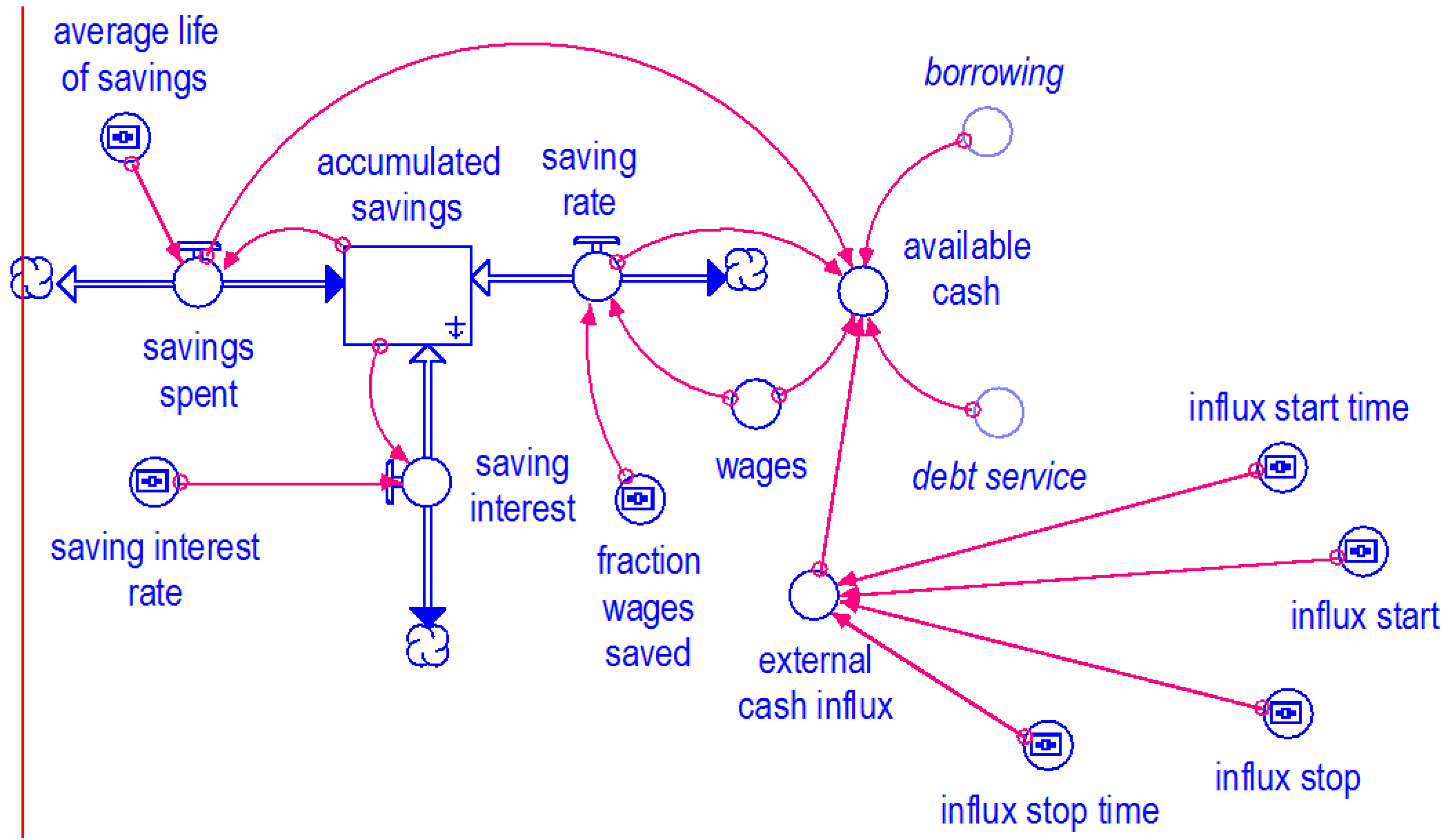
3.2. The Cash Available to Households
The cash available to households in each period, depicted in
Figure 3, can be spent or saved/invested. In
Figure 3, available cash for households to spend is a function of savings, income, borrowing, and the influx of cheap money. Specifically, it consists of their earnings, previous savings and borrowings less the debt served. In addition to these standard components, available cash also consists in the current model of cheap money. Thus, the equation for available cash in each time period t is as follows:
where
W is wage,
S is accumulated savings, β
s is the life of savings,
B is borrowing,
is fraction of debt serviced,
is the fraction of wage that is saved,
CM is cheap money. Therefore,
is the change in asset holdings across time
t to
t + 1 from the household balance sheet,
is the debt serviced and
are the current savings out of wages. Cheap money in Equation (5) becomes available to households due to government policies designed to encourage home ownership, e.g., the expansion of affordable housing mission of Freddie Mac and Fannie Mae, and the Community Reinvestment Act (CRA) [
2]. Another source of the cheap money arises as the price of the real estate assets of households rises and this creates new wealth for households, which they spend. [
10].
The accumulated savings of a household at time
t are adjusted according to the following equation:
where,
rs is the rate of interest on saving. Thus
are savings,
is the interest earned and
is the change in asset holdings across time
t to
t + 1 from the household balance sheet.
Figure 3.
Cash available to households.
Figure 3.
Cash available to households.
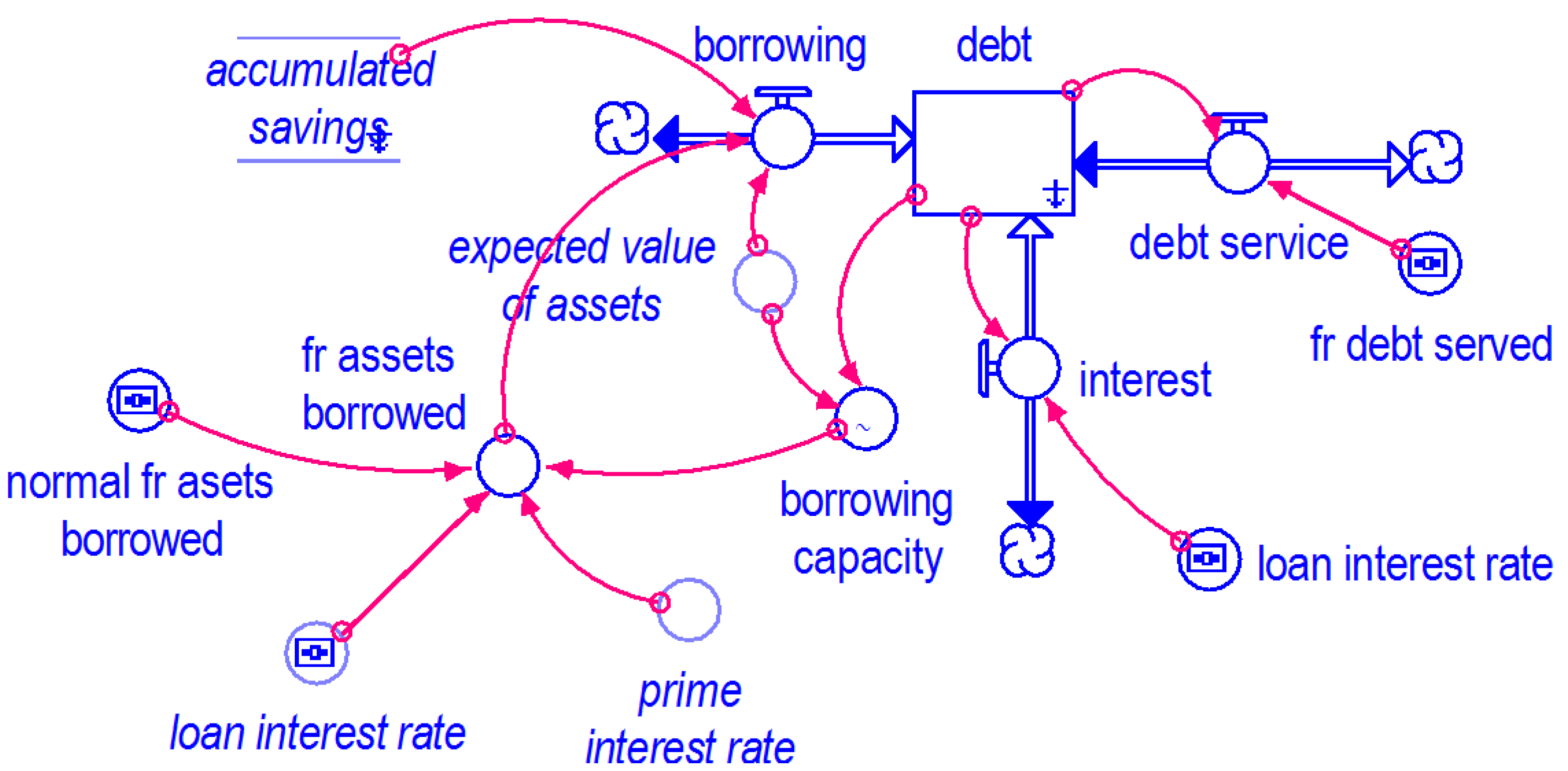
3.3. Household Debt
The evolution of households’ debt is illustrated in
Figure 4.
Figure 4 shows that household debt is determined by the borrowing capacity, interest rates, as well as the expected value of assets among other things. Households borrow a fraction of the total value of their assets in each time period
t. The fraction of assets borrowed by the household
i,
, is given by the following equation:
where
is household
i’s borrowing capacity,
is the normal fraction of asset value that is borrowed,
is the prime interest rate and
is the loan interest rate.
Borrowing capacity is a function of existing debt and the expected value of household assets as follows:
where the denominator of the right hand side,
, stands for the expected future value of assets. The household debt at time t is adjusted according to the following equation:
where
is the interest paid on loans and
is the debt service. Borrowing in time period
t equals:
where,
is the expected value of assets in the future. The normal fraction of assets borrowed had been rising before the housing market crisis. Indirect evidence of this is the sharp rise in actual US household debt in the run-up to the housing crisis (
Figure 6). This was in part the result of financial regulation not keeping up with financial innovation, which, in effect, loosened constraints on the banking sector’s capital requirements. The capability to repackage and sell home mortgage and other loans is an example of financial innovation that increased banks’ lending capacity with the same amount of capital. In addition, regulatory concessions such as allowing banks to use credit default swaps to reduce capital requirements starting in 1996 and permitting the large investment banks to self-determine capital requirements [
2].
Figure 4.
Household debt.
Figure 4.
Household debt.
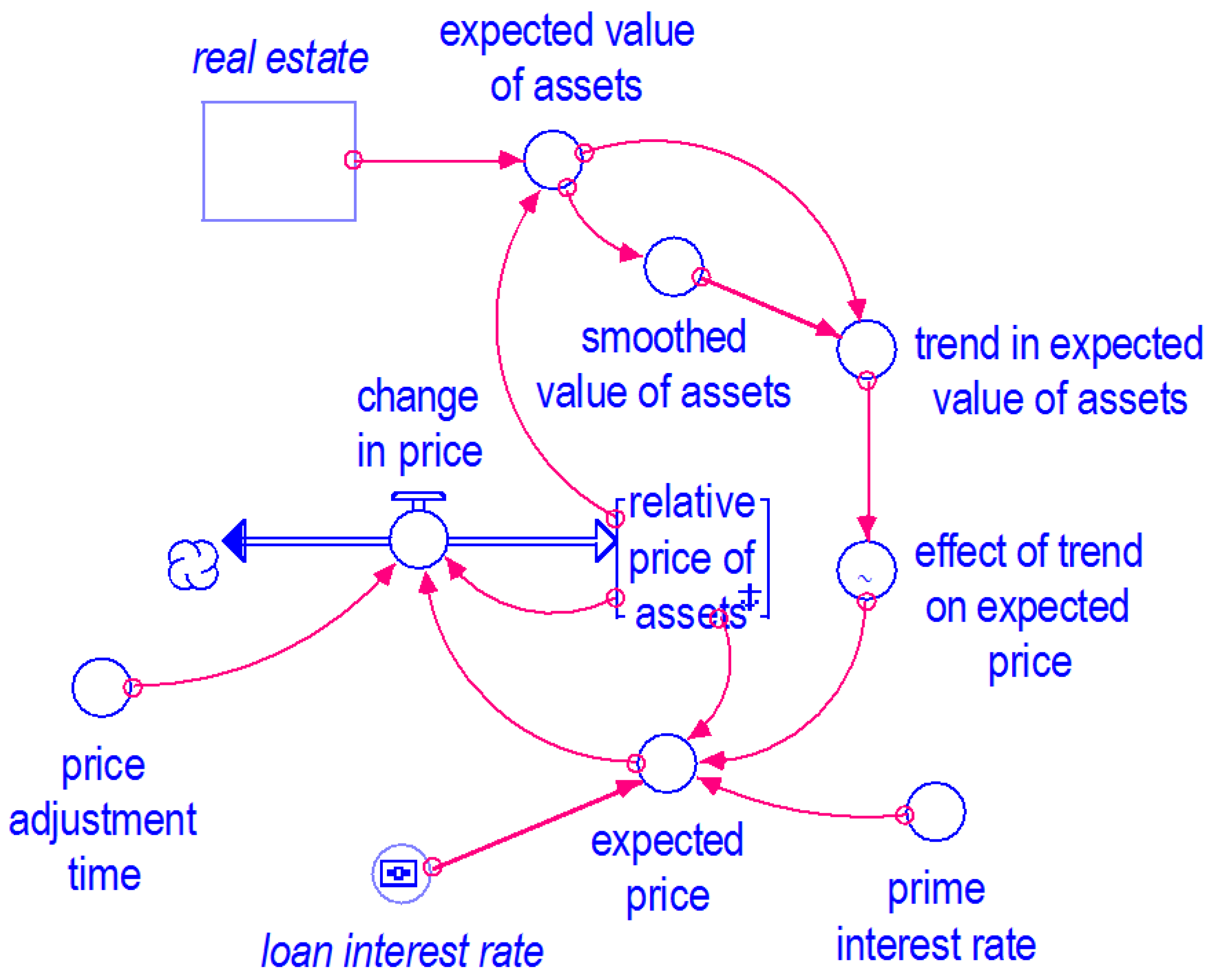
3.4. The Price of Real Estate
Figure 5 presents the process by which prices are determined. Price expectations of real estate are backward looking and self-fulfilling. Specifically, expected price is directly related to the past observed trend of prices in addition to the interest rate and the relative price of these assets. This formulation is shown in
Figure 5. It implies that an upward trend of home prices will generate future expectations of a continued rise. This is what was observed during the run-up in home prices. In
Figure 6 we see accelerating actual US home prices in the run up to the market crash, particularly up to 2005. Specifically the willingness of households to continue buying homes in the face of rising prices was driven in large part due to the expectation that prices would continue rising Bernanke [
2]. In our model the expectation turns out to be self-fulfilling as the price is assumed to move progressively in the direction of the expected price. The continued willingness of banks to lend and for households to invest into homes is believed to have lead to the persistent rise in home prices Levine and Bernanke [
1,
2].
The relative price of homes changes over time period t as follows:
where
is the expected price adjustment time and the expected price is as follows:
In Equation (12), the effect of trend on expected prices stands for the notion that expected price is backward looking. People expect the ongoing trend to continue. The trend is calculated as a ratio of the existing value of assets over the smoothed average. Specifically:
In Equation (13), is the existing volume of homes at time t. The denominator is a smoothed average value of assets calculated as a moving average of the two past time periods.
Figure 6.
Annual chart of indexed series.
Figure 6.
Annual chart of indexed series.
4. The Experiments
For the experiments section of our analysis we will follow the chronological order of the actual events that have been hypothesized to be the causes of the crisis. We conduct four experiments. Given their chronological nature, each experiment is overlaid atop the others that came before it as we move forward in time.
Our first experiment simulates the overly easy credit availability that resulted from the high importance designated to credit rating agencies and the failure of regulation to keep up with current financial innovation. In the second experiment, cheap money become available to households from abroad, as well as domestically from the government’s initiatives to increase home ownership. The third experiment simulates the expansionary monetary policy of low interest rates. The fourth simulates bankruptcy reform that in effect reduces the servicing of home mortgages.
In experiment 1 the fraction of assets borrowed by households increases (Equation (7)) due to lax financial regulations that result in excessive lending to households, in experiment 2 cheap money increases the cash that is available to households (Equation (5)), in experiment 3 interest rates are lowered by the Fed (Equation (6)) and kept low for a prolonged period of time and finally in experiment 4 bankruptcy reforms force households with financial troubles to put a smaller fraction of their tight finances towards servicing their mortgage debt than they would earlier have (Equation (9)).
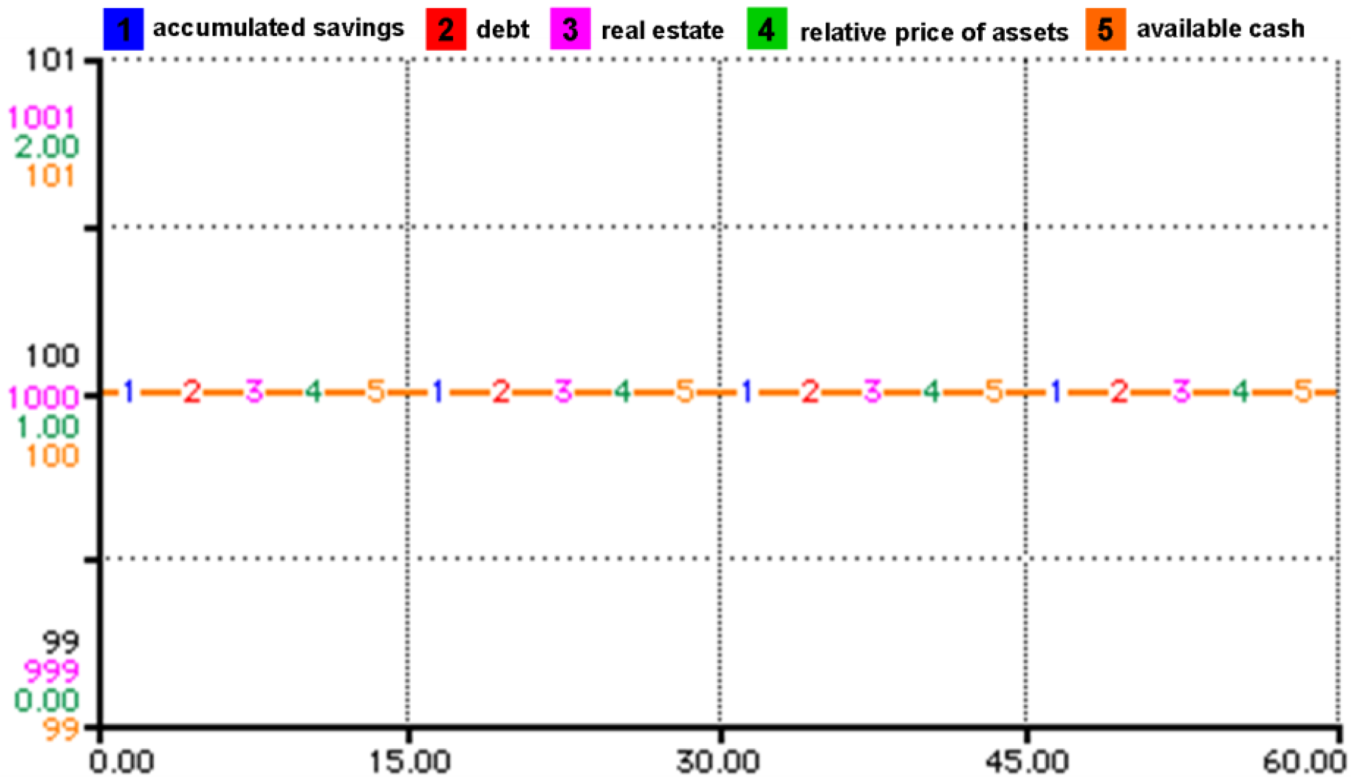
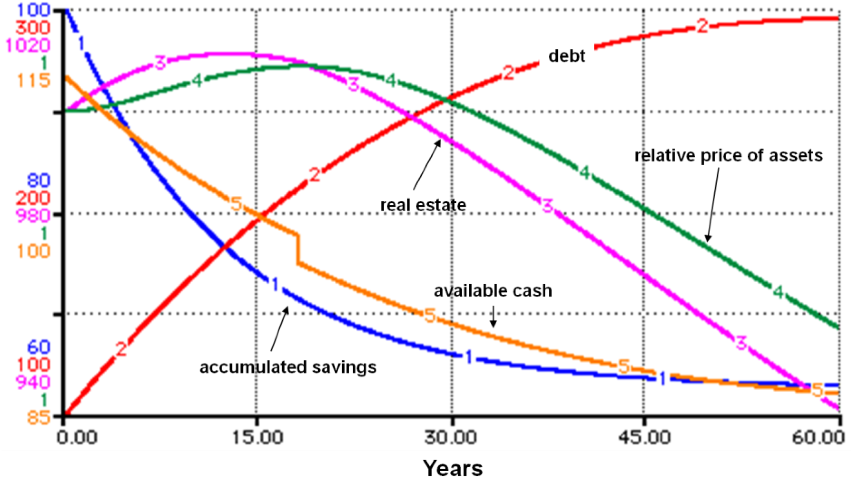
We begin with the market clearing equilibrium simulated in
Figure 7.
Table 2 contains the initial parameter values that ensure steady-state equilibrium. This serves as a point of reference since all stocks are in steady state. The equilibrium is dynamic, flows occur in every time period in such a way as to maintain stocks in their steady state. The initial steady-state equilibrium is used to illustrate the dynamics of the system. It is not calibrated to quantitatively produce any specific time history or forecast future. It is calibrated for initial equilibrium and its internal dynamics create the qualitative pattern representing the path to a new homeostasis when a policy parameter is changed. Each of our experiments alters the model’s parameter set and the model seeks a new equilibrium, but the primary point of interest is the path the system takes toward the new equilibrium that we attempt to describe.
Table 2.
Initial Parameter values *.
Table 2.
Initial Parameter values *.
| Parameter | Definition | Value |
|---|
| βH | Life of a real-estate asset | 50 |
| Normal fraction of cash invested by households | 0.2 |
| βs | Average life of savings | 10 |
| αWS | Fraction of wages saved | 0.05 |
| rs | Savings interest rate | 0.05 |
| W | Wages | 100 |
| αD | Fraction of debt served | 0.1 |
| rloan | Loan interest rate | 0.05 |
| Normal fraction of assets borrowed | 5/1100 |
| μp | Price adjustment time | 2 |
| rprime | Prime interest rate | 0.05 |
Figure 7.
Market clearing equilibrium.
Figure 7.
Market clearing equilibrium.
4.1. Experiment 1: Lax Financial Regulations
Our first experiment corresponds to lax financial regulations. This movement started as far back as 1975 when credit rating agencies were given NSRO status, gathered momentum in 1996 when CDSs were permitted in lieu of bank capital and was further reinforced in 2004 when investment banks were allowed to determine their own capital. In our model the lax financial regulation leads to lax rules for household borrowing. Specifically, it is represented by an increase in the normal fraction of assets borrowed by the households in Equation (7). There is support for this formulation in the actual data from the housing crisis. There was a rapid increase in mortgages with non-standard features that made them initially affordable;
Table 3 presents evidence of their increase. In addition,
Figure 6 shows the sharp and accelerated increase in actual household debt.
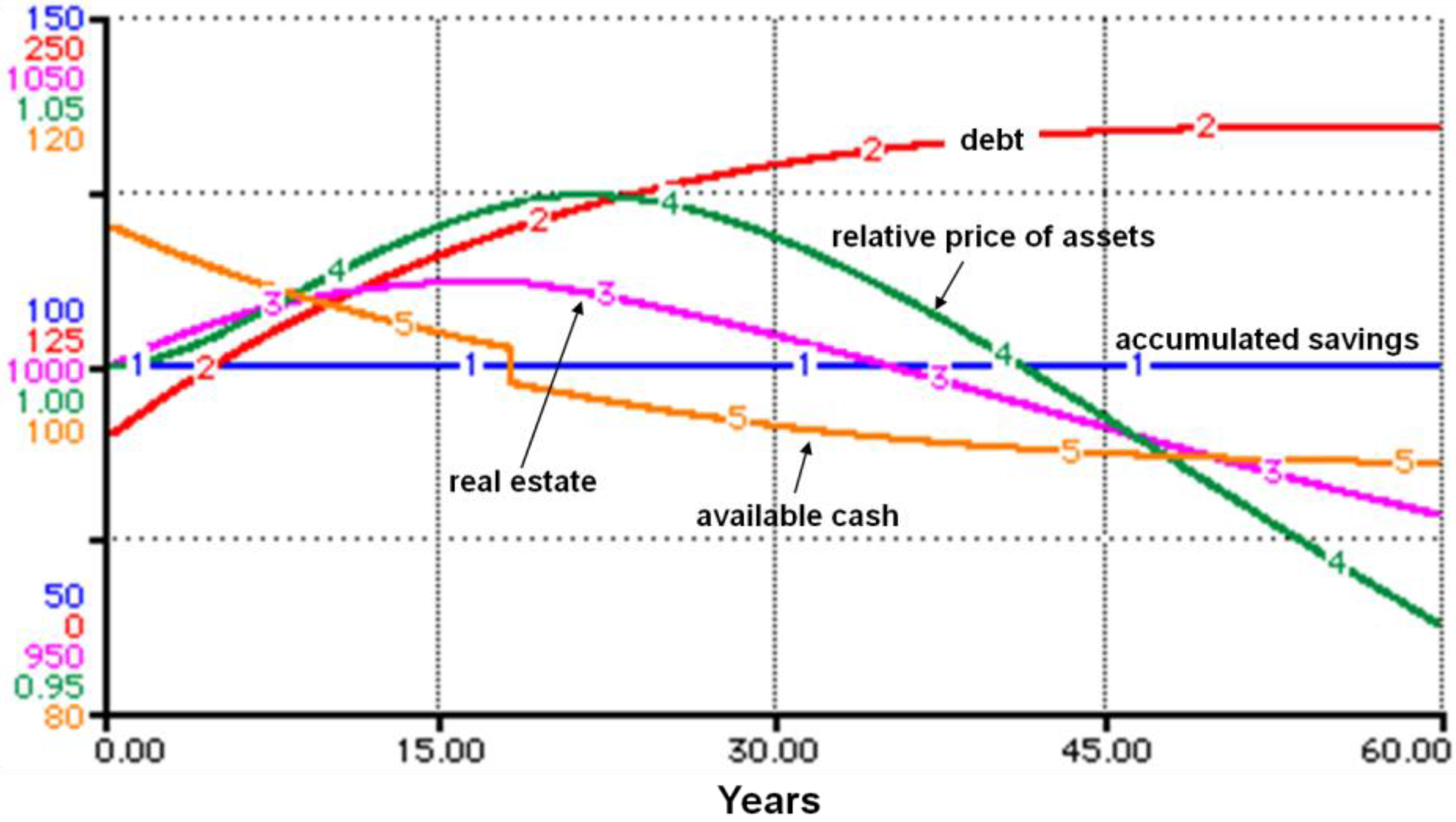
The normal fraction of assets borrowed by households at steady state is 0.5 percent of total assets in
Table 2. This is doubled in the experiment to one percent. The results are shown in
Figure 8. Housing prices rise at an accelerated pace in the first 18 time periods. After time period 18, they fall at an accelerating pace. This matches with actual data surrounding the housing crisis shown in
Figure 6. The run up to the crisis home price rise was accelerating and once home prices started falling, this fall was accelerating as well.
Table 3.
Financial innovation in mortgages (as a percentage of adjustable rate mortgage originated in that year).
Table 3.
Financial innovation in mortgages (as a percentage of adjustable rate mortgage originated in that year).
| | Interest Only * | Extended Amortization * | Negative Amortization * | Pay Option * |
|---|
| | Subprime | Alt-A | Subprime | Alt-A | Alt-A | Alt-A |
|---|
| 2000 | 0 | 3 | 0 | 0 | | |
| 2001 | 0 | 8 | 0 | 0 | | |
| 2002 | 2 | 37 | 0 | 0 | | |
| 2003 | 5 | 48 | 0 | 0 | 19 | 11 |
| 2004 | 18 | 51 | 0 | 0 | 40 | 25 |
| 2005 | 21 | 48 | 13 | 0 | 46 | 38 |
| 2006 | 16 | 51 | 33 | 2 | 55 | 38 |
Figure 8.
Experiment 1—lax financial regulation.
Figure 8.
Experiment 1—lax financial regulation.
This result arises due to the extra borrowing undertaken by households in order to invest in homes. Home prices rise as demand for home purchases increases. As prices rise, this trend is self-reinforcing because price changes are backward looking in our model (Equation (12)). Therefore price rise accelerates over time. To add further fuel to this process, this increase in prices feeds back into household investment behavior due to the fact that the fraction of cash that is available to households that they choose to invest in homes is dependent on the current trend in home prices (Equation (4)). Therefore, as home prices rise, so do the investment in homes.
House prices finally start falling as the household debt builds up and the debt service burden finally makes it harder for households to sustain ever-higher levels of real estate investment (Equation (5)). This puts the brakes on real estate prices, and finally leads to a fall in prices as demand evaporates. As before, the price trend is self-reinforcing, only this time the direction of change is downward as the fall in real estate prices is feeds on itself (Equation (12)). In actual data,
Figure 6, we see that household debt keeps rising even after the housing crash, house prices start falling in 2007, while it is only in 2009 that household debt finally starts falling.
4.2. Experiment 2: Influx of Cheap Money
The second experiment corresponds to cheap money that became available to households in the face of already increased borrowing from lax financial regulations. The cheap money became available through at least two sources: the savings glut in developing countries particularly following the Asian crisis of 1997–1998 Bernanke [
3]; and the government policy geared towards encouraging home ownership through expansion of affordable housing mission of the GSEs and the Community Reinvestment Act. In
Figure 6 the actual data corroborates this experiment as household expenditure increased faster in the run up to the crisis indicating an increase in cash available for households to spend.
In our model the savings glut and government’s encouraging of home ownership manifest themselves through an influx of “cheap money” into the available cash pool of the household (Equation (5)). The cheap money comes in through the channel of credit to households, however as soon as the crisis hits this money dries up as the economy’s credit mechanism freezes. This is what happened in the US housing crisis as banks stopped lending and the credit crunch hit following the start of the housing crisis. In
Figure 6, we see this as a mild fall in actual expenditure and the eventual falling of household debt after the crisis. Notice how actual expenditure and debt reduction lag the falling home prices. This provides some support for our findings.
Results are shown in
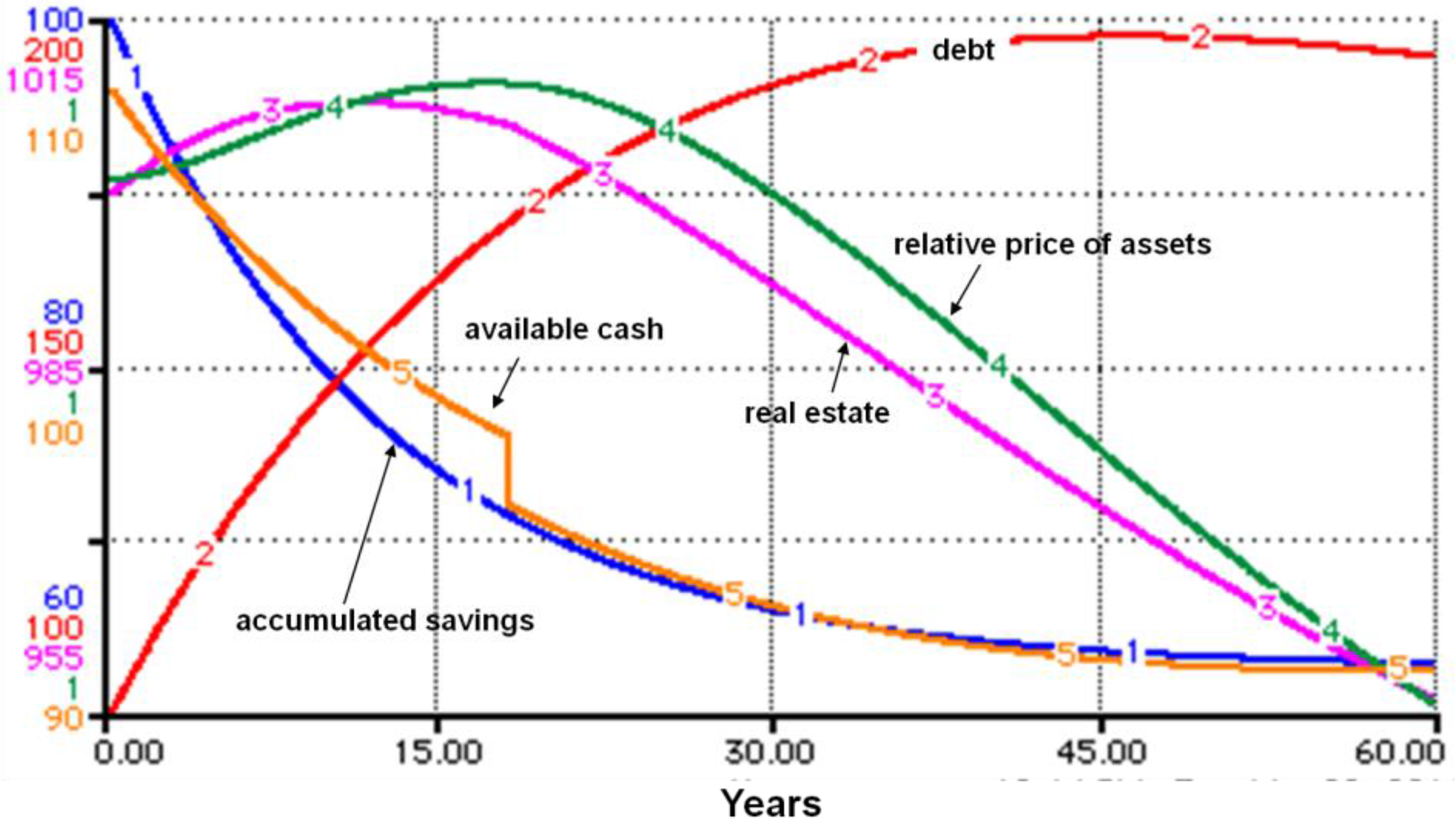
Figure 9. We assume that the influx of cheap money starts at time period 0 and stops at time period 18. Recall that the housing prices started falling in time period 18 in the first experiment. Thus to replicate the real world situation where credit dried up as the housing crisis hit, we stop the influx at time period 18.
This result indicates that this extra cash helps households to invest even more in homes. Home prices rise even higher and remain elevated for longer period of time. The fall in home prices starts only around time period 22. The reasons for the fall are similar to the ones in the first experiment. Households’ borrowing capacity falls due to increased indebtedness; although in the second experiment this fall comes later because the availability of cheap money helps to enhance the household’s debt servicing capacity for longer. Another important difference is that home prices fall less than before. This is because even though the influx of cheap money has ceased, it has served to support household finances by keeping borrowing costs low for a period of time.
Figure 9.
Experiment 2—cheap money inflow (and experiment 1).
Figure 9.
Experiment 2—cheap money inflow (and experiment 1).
4.3. Experiment 3: Lowering Interest Rates
The Federal Reserve lowered their target interest rate starting in 2001 in order to stabilize the economy in the face of the recession in the economy at that time. Following the 11 September 2001 terrorist attacks in New York, unemployment and corporate scandals, the Federal Reserve kept interest rates at that low level for most of the early part of the decade. Many have cited this as the cause for the housing bubble as low mortgage interest rates might have led households to borrow excessively and invest in homes that would have been out of their reach at higher interest rates.
Table 2 indicates our steady state equilibrium savings interest rates as 5% we decrease this to 2% in this experiment. We leave the loan interest rate unchanged since the second experiment depicts a de-facto lowering of this interest via the availability of cheap money. As before, we conduct experiment 3 in conjunction with the conditions prevailing under experiments 1 and 2. Thus, the normal fraction of assets borrowed is elevated and so is the cheap money influx to households up to period 18.
The results indicate that the boom in the housing market is comparable to the first experiment. The housing prices rise in similar fashion: at much the same rate and for about the same period of time. However in the new experiment the fall is much more precipitous and house prices end up at a significantly lower level.
The results in
Figure 10 add at least two substantive new findings to the previous experiments. First, in spite of cheap money influx, the housing price boom is not as large as experiment two. This is directly linked to another outcome of the third experiment that household savings are lower in this case than before. The reason can be traced to the low interest rate regime. In this experiment even though cheap money still flows in households’ own accumulated savings take a dip (Equation (6)). The second new finding is that there is a greater fall in house prices compared to earlier experiments. This result is also directly related to lower household savings because of lower interest rates.
Figure 10.
Impact of low interest rates due to expansionary monetary policy (and experiments 1 and 2).
Figure 10.
Impact of low interest rates due to expansionary monetary policy (and experiments 1 and 2).
This is an interesting result in many ways. There has been much argument about the role of the Fed in creating the crisis and the Fed has defended its low interest rate stance in the early 2000s as not being the cause of the housing crisis Bernanke [
2]. The results of our experiment show a new dimension in this argument. It findings seem to support the Fed in its stance that low interest rates did not feed the bubble. We see in the third experiment that home prices actually grew at a slower pace and did not reach the highs that it would have reached in the absence of low interest rates. Interestingly the reason our model renders this result is contrary to the arguments presented by the Federal Reserve in terms of “savings glut” from abroad. Our findings indicate that low savings resulting from low interest rates drives this result. The languishing actual savings is depicted in
Figure 6, savings only start recovering after the housing crash. In addition once home prices start falling the Fed’s low interest rate stance makes the crisis worse as housing prices fall further than they otherwise would have. The literature, as well as the Federal Reserve’s own energies, have been concentrated in trying to explain the role of low interest rates as having encouraged home ownership and therefore inflated house prices. However, the results of this experiment show that in the context of the previously existing conditions such as lax financial regulations (experiment 1) and the availability of cheap money for households (experiment 2), the Federal Reserve’s role was most important in reducing household savings.
4.4. Experiment 4: Mortgage Reform
Our final experiment simulated in
Figure 11 attempts to demonstrate the impact of mortgage reform of 2005. This reform made it harder for households to apply for bankruptcy by raising the cost of filing. In addition it gave limited protection from creditors compared to before. This meant that where households could have chosen to concentrate their finances in servicing mortgage debt to keep their home, now they were forced to service other debt as well. This reduced the amount of mortgage debt that could be served by them [
6].
Figure 11.
Experiment 4: Adding bankruptcy reform to experiments 1, 2 and 3.
Figure 11.
Experiment 4: Adding bankruptcy reform to experiments 1, 2 and 3.
Since the only asset in our model is real estate, this experiment corresponds to a reduction in the fraction of debt served in Equation (9). From
Table 2, the equilibrium fraction of debt served is 10%, this is lowered to 8% for this experiment. The results indicate that the rise in home prices is similar to experiment 2. However the fall is much greater than earlier experiments as the number of defaults rises due to lower debt service.
This result supports the mechanism hypothesized in the literature, which estimates that the 2005 reform caused mortgage default rates to rise 14 percent for prime borrowers and 16 percent for subprime borrowers. The literature has estimated that this increase in default rates, which began before the current mortgage crisis, has generated roughly 200,000 additional defaults each year, and exacerbated the housing crisis [
6].
4.5. Summing up the Experiments
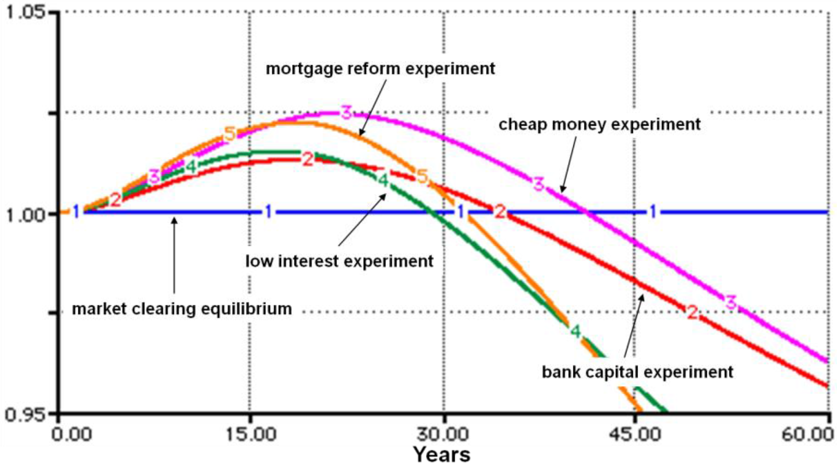
Figure 12 presents a comparative graph of housing price in each experiment. It brings into focus the causes, cited in the literature, that explain the bubble in the housing market,
i.e., the boom and then the bust in home prices in the US. We see that some of the causes fit neatly into the role of creating this boom and bust pattern of housing prices. Our first experiment that dealt with the lax financial regulation, for example, clearly leads to this outcome. There is an initial price rise followed by an accelerated price fall. The remaining three experiments, however, provide mixed results. The causes of crisis that they represent do not always create the entire boom bust pattern. In the second experiment, the influx of cheap money, amplifies the boom,
i.e., it leads to an even greater price rise that persists for a longer period of time, thus magnifying the bubble on the upswing. However it cushions the fall in prices, as house prices fall less. In the third experiment, low interest rates, lead to greater downturn in prices, however it actually dampens the initial price rise due to low household savings available for investment. Similarly bankruptcy reform depicted in the fourth experiment also leads to a more pronounced downturn. This is because mortgage reform reduces the households’ capacity to service their debt.
Figure 12.
Comparison of housing prices across all experiments.
Figure 12.
Comparison of housing prices across all experiments.


