The Bifactor Model Fits Better Than the Higher-Order Model in More Than 90% of Comparisons for Mental Abilities Test Batteries

Abstract
:1. Introduction
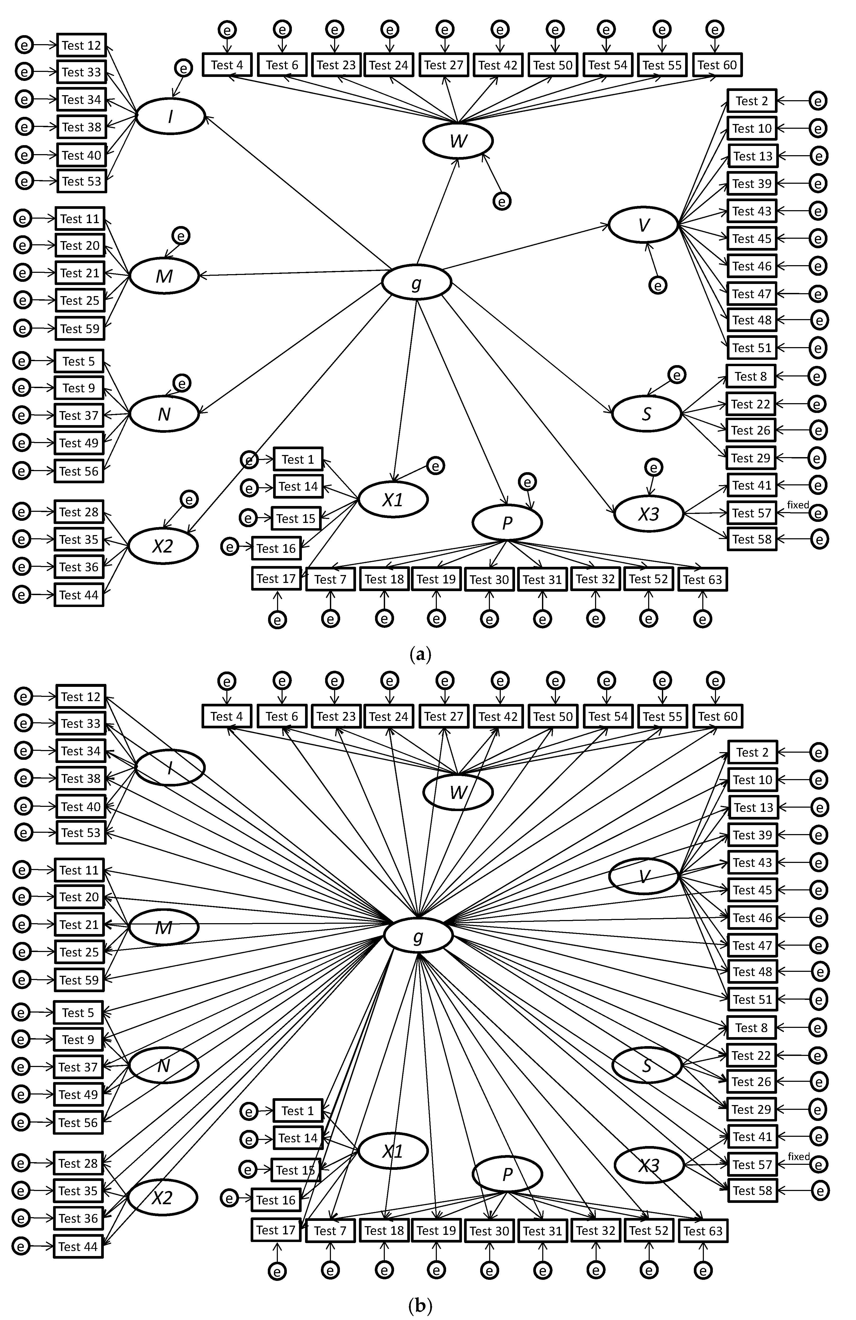
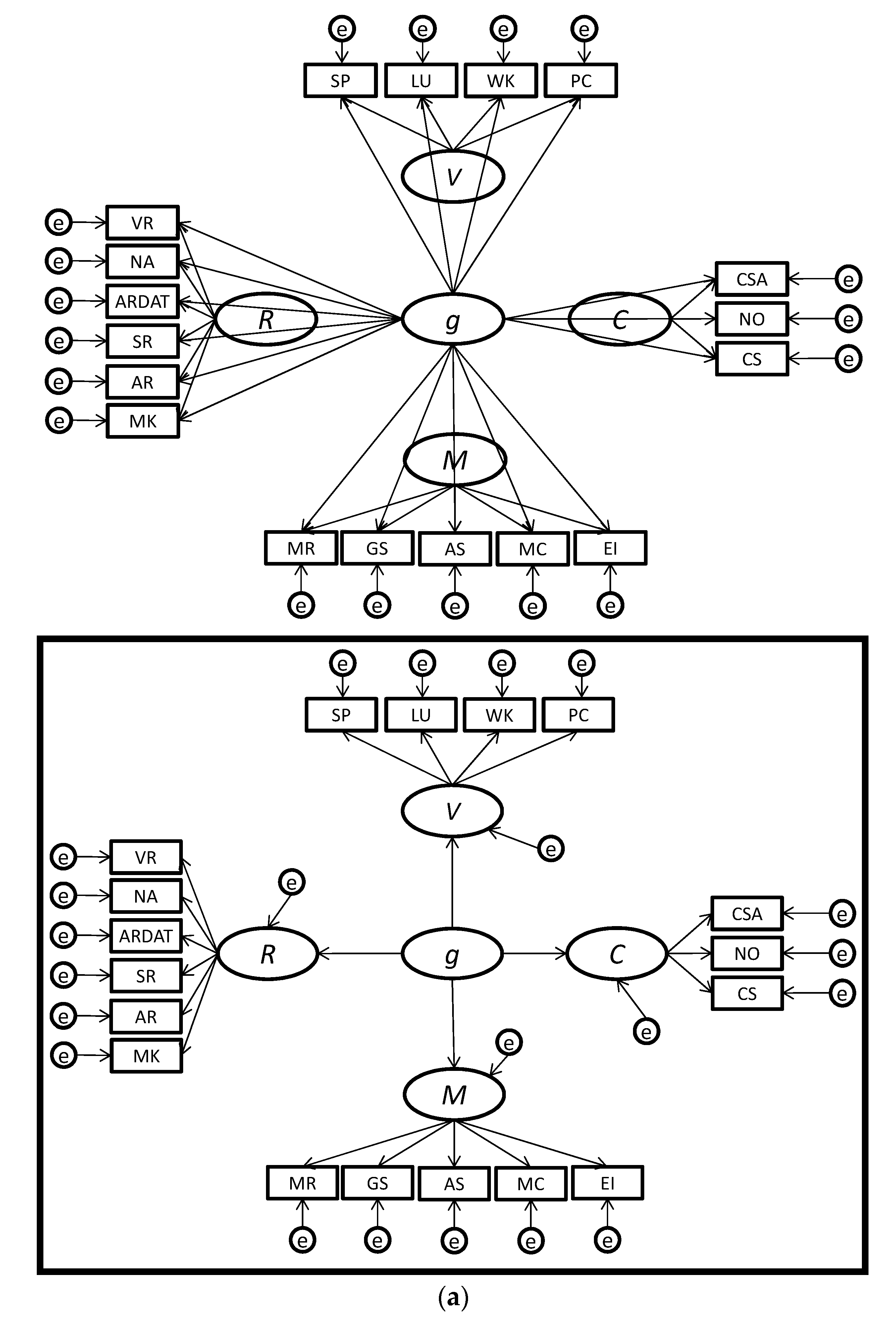
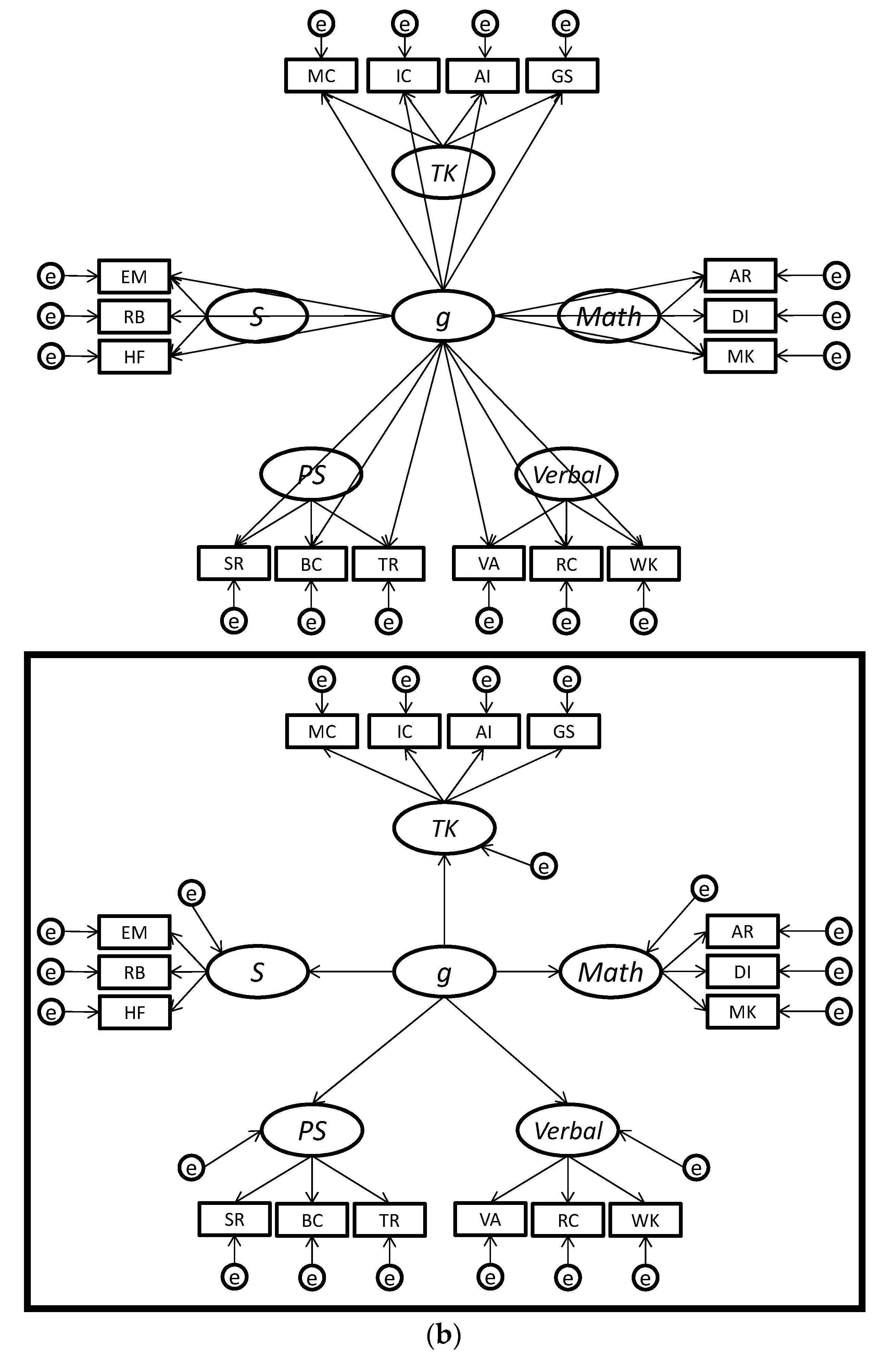
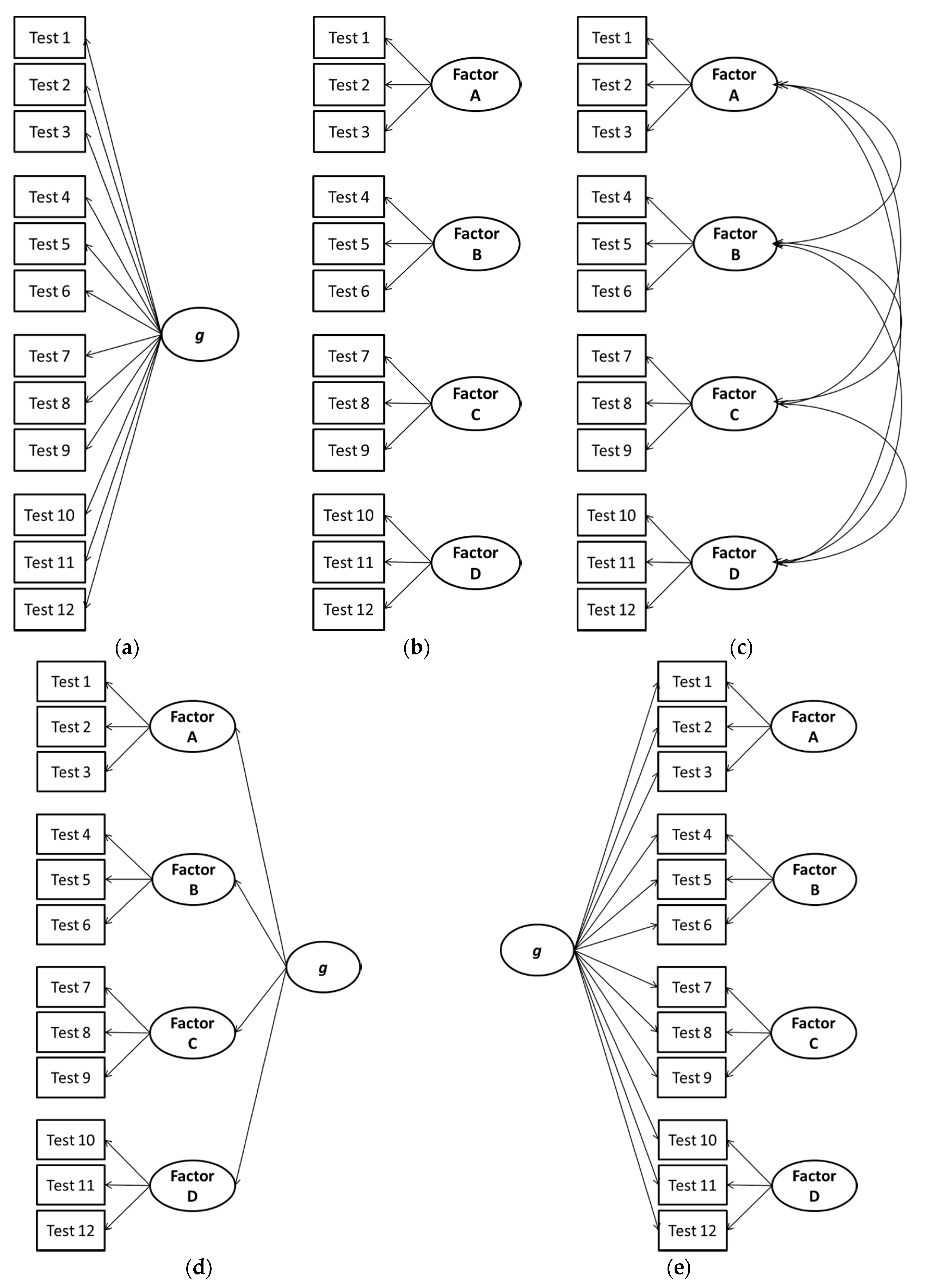
1.1. Higher-Order Model
1.2. Bifactor Model
1.3. Model Building
1.4. Past Research and the Need for Further Research
2. Materials and Methods
2.1. Selection of Datasets
2.2. Test Batteries and Datasets
2.3. Data Analysis Approach/Philosophy
3. Results
3.1. Additional Analyses
3.2. Summary of Results
4. Discussion
4.1. Loading Interpretation Considerations with the Higher-Order and Bifactor Models
4.2. Proportionality Considerations with the Higher-Order and Bifactor Models
4.3. Parsimony Considerations with the Higher-Order and Bifactor Models
4.4. Is the Higher-Order Model a Remnant of an Antiquated Compromise?
4.5. Limitations and Future Research
Supplementary Materials
Acknowledgments
Author Contributions
Conflicts of Interest
References
- American Educational Research Association, American Psychological Association, and National Council on Measurement in Education. Standards for Educational and Psychological Testing; American Educational Research Association: Washington, DC, USA, 2014. [Google Scholar]
- Bollen, K.; Lennox, R. Conventional wisdom on measurement: A structural equation perspective. Psychol. Bull. 1991, 110, 305–314. [Google Scholar] [CrossRef]
- Holzinger, K.; Swineford, F. The Bi-factor method. Psychometrika 1937, 2, 41–54. [Google Scholar] [CrossRef]
- Holzinger, K.; Swineford, F. A study in factor analysis: The stability of a bifactor solution. In Supplementary Educational Monograph; No. 48; University of Chicago Press: Chicago, IL, USA, 1939. [Google Scholar]
- Reeve, C.L.; Blacksmith, N. Identifying g: A review of current factor analytic practices in the science of mental abilities. Intelligence 2009, 37, 487–494. [Google Scholar] [CrossRef]
- Jensen, A.R. The g Factor: The Science of Mental Ability; Praeger Publishers: Westport, CT, USA, 1998. [Google Scholar]
- Jensen, A.R.; Weng, L. What is a good g? Intelligence 1994, 18, 231–258. [Google Scholar] [CrossRef]
- Thurstone, L.L.; Thurstone, T.G. Factorial studies of intelligence. Psychom. Monogr. 1941, 2, 1–94. [Google Scholar]
- Carroll, J.B. Human Cognitive Abilities: A Survey of Factor Analytic Studies; Cambridge University Press: New York, NY, USA, 1993. [Google Scholar]
- Beaujean, A.A. John Carroll’s views on intelligence: Bi-factor vs. higher-order models. J. Intell. 2015, 3, 121–136. [Google Scholar] [CrossRef]
- Gignac, G.E. Revisiting the factor structure of the WAIS-R: Insights through nested factor modeling. Assessment 2005, 12, 320–329. [Google Scholar] [CrossRef] [PubMed]
- Gignac, G.E. A confirmatory examination of the factor structure of the Multidimensional Aptitude Battery: Contrasting oblique, higher order, and nested factor models. Educ. Psychol. Meas. 2006, 66, 136–145. [Google Scholar] [CrossRef]
- Gignac, G.E. The WAIS-III as a nested factors model: A useful alternative to the more conventional oblique and higher-order models. J. Individ. Differ. 2006, 27, 73–86. [Google Scholar] [CrossRef]
- Gignac, G.E. Higher-order models versus direct hierarchical models: g as superordinate or breadth factor? Psychol. Sci. Q. 2008, 50, 21–43. [Google Scholar]
- Collinson, R.; Evans, S.; Wheeler, M.; Brechin, D.; Moffitt, J.; Hill, G.; Muncer, S. Confirmatory factor analysis of WAIS-IV in a clinical sample: Examining a bi-factor model. J. Intell. 2016, 5, 2. [Google Scholar] [CrossRef]
- Reise, S.P. The rediscovery of bifactor measurement models. Multivar. Behav. Res. 2012, 47, 667–696. [Google Scholar] [CrossRef] [PubMed]
- Reynolds, M.R.; Keith, T.Z. Spearman’s law of diminishing returns in hierarchical models of intelligence for children and adolescents. Intelligence 2007, 35, 267–281. [Google Scholar] [CrossRef]
- Murray, A.L.; Johnson, W. The limitations of model fit in comparing the bi-factor versus higher-order models of human cognitive ability structure. Intelligence 2013, 41, 407–422. [Google Scholar] [CrossRef]
- Gignac, G.E. The higher-order model imposes a proportionality constraint: That is why the bifactor model tends to fit better. Intelligence 2016, 55, 57–68. [Google Scholar] [CrossRef]
- Mansolf, M.; Reise, S.P. When and why the second-order and bifactor models are distinguishable. Intelligence 2017, 61, 120–129. [Google Scholar] [CrossRef]
- Beaujean, A.A.; Parkin, J.; Parker, S. Comparing Cattell-Horn-Carroll factor models: Differences between bifactor and higher order factor models in predicting language achievement. Psychol. Assess. 2014, 26, 789–805. [Google Scholar] [CrossRef] [PubMed]
- Benson, N.; Hulac, D.M.; Bernstein, J.D. An independent confirmatory factor analysis of the Wechsler Intelligence Scale for Children—Fourth Edition (WISC-IV) Integrated: What do the process approach subtests measure? Psychol. Assess. 2013, 25, 692–705. [Google Scholar] [CrossRef] [PubMed]
- Gignac, G.E.; Watkins, M.W. Bifactor modeling and the estimation of model-based reliability in the WAIS-IV. Multivar. Behav. Res. 2013, 48, 639–662. [Google Scholar] [CrossRef] [PubMed]
- Golay, P.; Lecerf, T. Orthogonal higher order structure and confirmatory factor analysis of the French Wechsler Adult Intelligence Scale (WAIS–III). Psychol. Assess. 2011, 23, 143–152. [Google Scholar] [CrossRef] [PubMed]
- Niileksela, C.R.; Reynolds, M.R.; Kaufman, A.S. An alternative Cattell-Horn-Carroll (CHC) factor structure of the WAIS-IV: Age invariance of an alternative model for ages 70–90. Psychol. Assess. 2013, 25, 391–404. [Google Scholar] [CrossRef] [PubMed]
- Von Stumm, S.; Chamorro-Premuzic, T.; Quiroga, M.A.; Colom, R. Separating narrow and general variances in intelligence-personality associations. Personal. Individ. Differ. 2009, 47, 336–341. [Google Scholar] [CrossRef]
- Brown, T.A. Confirmatory Factor Analysis for Applied Research; The Guilford Press: New York, NY, USA, 2006. [Google Scholar]
- Mueller, R.O. Basic Principles of Structural Equation Modeling: An Introduction to LISREL and EQS; Springer: New York, NY, USA, 1999. [Google Scholar]
- Wechsler, D. Wechsler Adult Intelligence Scale—Fourth Edition; Pearson Assessment: San Antonio, TX, USA, 2008. [Google Scholar]
- Wechsler, D. Wechsler Adult Intelligence Scale—Revised; Psychological Corporation: New York, NY, USA, 1981. [Google Scholar]
- Wechsler, D. WAIS-III WMS-III Technical Manual; Psychological Corporation: San Antonio, TX, USA, 1997. [Google Scholar]
- Jackson, D.N. Multidimensional Aptitude Battery: Manual; Research Psychologist Press: Port Huron, MI, USA, 1984. [Google Scholar]
- Jackson, D.N. Multidimensional Aptitude Battery—II: Manual; Sigma Assessment Systems: Port Huron, MI, USA, 1998. [Google Scholar]
- Colom, R.; Rebollo, I.; Palacios, A.; Juan-Espinosa, M.; Kyllonen, P.C. Working memory is (almost) perfectly predicted by g. Intelligence 2004, 32, 277–296. [Google Scholar] [CrossRef]
- Gustafsson, J.-E. A unifying model for the structure of intellectual abilities. Intelligence 1984, 8, 179–203. [Google Scholar]
- Gustafsson, J.-E. On the hierarchical structure of ability and personality. In Intelligence and Personality: Bridging the Gap in Theory and Measurement; Collis, J.M., Messick, S., Eds.; Erlbaum: Mahwah, NJ, USA, 2001; pp. 25–42. [Google Scholar]
- Raven, J.C. Progressive Matrices: A Perceptual Test of Intelligence; H.K. Lewis: London, UK, 1938. [Google Scholar]
- Yela, M. Solid Figures Rotation; TEA: Madrid, Spain, 1969. [Google Scholar]
- Thurstone, L.L. Primary Mental Abilities; University of Chicago Press: Chicago, IL, USA, 1938. [Google Scholar]
- The Psychological Corporation. Differential Aptitude Tests for Personnel and Career Assessment: Technical Manual; Psychological Corporation: San Antonio, TX, USA, 1991. [Google Scholar]
- Bennett, G.K.; Seashore, H.G.; Wesman, A.G. Differential Aptitude Tests, 5th ed.; Psychological Corporation: San Antonio, TX, USA, 1990. [Google Scholar]
- Golay, P.; Reverte, I.; Rossier, J.; Favez, N.; Lecerf, T. Further insights on the French WISC-IV factor structure through Bayesian structural equation modeling. Psychol. Assess. 2013, 25, 496–508. [Google Scholar] [CrossRef] [PubMed]
- Morgan, G.B.; Hodge, K.J.; Wells, K.E.; Watkins, M.W. Are fit indices biased in favor of bi-factor models in cognitive ability research? A comparison of fit in correlated factors, higher-order, and bi-factor models via Monte Carlo simulations. J. Intell. 2015, 3, 2–20. [Google Scholar] [CrossRef]
- McGrew, K.S. Human Cognitive Abilities (HCA) Data Set Archive: Archiving of Carroll’s 1993 Data Sets, 2011. Available online: http://www.iapsych.com/wmfhcaarchive/wmfhcaindex.html (accessed on 7 July 2017).
- McGrew, K.S.; Flanagan, D.P. The Intelligence Test Desk Reference (ITDR): The Gf-Gc Cross-Battery Assessment; Allyn & Bacon: Boston, MA, USA, 1998. [Google Scholar]
- McGrew, K.S. CHC theory and the human cognitive abilities project: Standing on the shoulders of the giants of psychometric intelligence research. Intelligence 2009, 37, 1–10. [Google Scholar] [CrossRef]
- Kettner, N. Armed Services Vocational Aptitude Battery (ASVAB Form 5): Comparison with GATB and DAT Tests; Technical Research Report No. 77–1; Military Enlistment Processing Command, Directorate of Testing: Fort Sheridan, IL, USA, 1977. [Google Scholar]
- Ree, M.J.; Earles, J.A. Predicting training success: Not much more than g. Pers. Psychol. 1991, 44, 321–332. [Google Scholar] [CrossRef]
- Ree, M.J.; Earles, J.A.; Teachout, M. Predicting job performance: Not much for than g. J. Appl. Psychol. 1994, 79, 518–524. [Google Scholar] [CrossRef]
- Cucina, J.M.; Peyton, S.T.; Su, C.; Byle, K.A. Role of Mental Abilities and Mental Tests in Explaining High-School Grades. Intelligence 2016, 54, 90–104. [Google Scholar] [CrossRef]
- Glutting, J.J.; Watkins, M.W.; Konold, T.R.; McDermott, P.A. Distinctions Without a Difference The Utility of Observed Versus Latent Factors From the WISC-IV in Estimating Reading and Math Achievement on the WIAT-II. J. Spec. Educ. 2006, 40, 103–114. [Google Scholar] [CrossRef]
- Yung, Y.F.; Thissen, D.; McLeod, L.D. On the relationship between the higher-order factor model and the hierarchical factor model. Psychometrika 1999, 64, 113–128. [Google Scholar] [CrossRef]
- Yang, R.; Spirtes, P.; Scheines, R.; Reise, S.P.; Mansolf, M. Finding Pure Submodels for Improved Differentiation of Bifactor and Second-Order Models. Struct. Equ. Model. 2017, 24, 402–413. [Google Scholar] [CrossRef]
- Kummerfeld, E.; Ramsey, J. Causal clustering for 1-factor measurement models. In Proceedings of the 22nd International Conference on Knowledge Discovery and Data Mining, San Francisco, CA, USA, 13–17 August 2016. [Google Scholar]
- Kummerfeld, E.; Ramsey, J.; Yang, R.; Spirtes, P.; Scheines, R. Causal clustering for 2-factor measurement models. In Machine Learning and Knowledge Discovery in Databases; Calders, T., Esposito, F., Hüllermeier, E., Meo, R., Eds.; Springer: New York, NY, USA, 2014; pp. 34–49. [Google Scholar]
- Lucas, C.M.; French, J.W. A Factorial Study of Experimental Tests of Integration, Judgment, and Planning; (Research Bulletin 53–16); Educational Testing Service: Princeton, NJ, USA, 1953. [Google Scholar]
- Reeve, C.L.; Bonaccio, S. The nature and structure of “intelligence”. In The Wiley Blackwell Handbook of Individual Differences; Chamorro-Premuzic, T., von Stumm, S., Furnham, A., Eds.; John Wiley & Sons, Ltd.: Malden, MA, USA, 2011; pp. 187–216. [Google Scholar]
- Gustafsson, J.E. Hierarchical models of individual differences in cognitive abilities. In Advances in the Psychology of Human Intelligence; Stemberg, R.J., Ed.; Lawrence Erlbaum Associates, Inc.: Hillsdale, NJ, USA, 1988; Volume 4, pp. 35–71. [Google Scholar]
- Gustafsson, J.E. Broad and narrow abilities in research on learning and instruction. In Abilities, Motivation, and Methodology. The Minnesota Symposium on Learning and Individual Differences; Kanfer, R., Ackermari, P.L., Cudeck, R., Eds.; Erlbaum: Hillsdale, NJ, USA, 1989; pp. 203–237. [Google Scholar]
- Gustafsson, J.-E. Measurement from a hierarchical point of view. In The Role of Constructs in Psychological and Educational Measurement; Braun, H.I., Jackson, D.N., Wiley, D.E., Eds.; Lawrence Erlbaum Associates, Publishers: Mahwah, NJ, USA, 2002; pp. 73–95. [Google Scholar]
- Cucina, J.M.; Howardson, G.N. Woodcock-Johnson-III, KAIT, KABC, and DAS support Carroll but not Cattell-Horn. Psychol. Assess. [CrossRef]
- Canivez, G.L. Bifactor modeling in construct validation of multifactored tests: Implications for multidimensionality and test interpretation. In Principles and Methods of Test Construction: Standards and Recent Advancements; Schweizer, K., DiStefano, C., Eds.; Hogrefe: Gottingen, Germany, 2016; pp. 247–271. [Google Scholar]
- Chen, F.F.; Hayes, A.; Carver, C.S.; Laurenceau, J.P.; Zhang, Z. Modeling general and specific variance in multifaceted constructs: A comparison of the bifactor model to other approaches. J. Pers. 2012, 80, 219–251. [Google Scholar] [CrossRef] [PubMed]
- Schmid, J.; Leiman, J.M. The development of hierarchical factor solutions. Psychometrika 1957, 22, 53–61. [Google Scholar] [CrossRef]
- Colom, R.; Abad, F.J.; Garcia, L.F.; Juan-Espinosa, M. Education, Wechsler’s full scale IQ, and g. Intelligence 2002, 30, 449–462. [Google Scholar] [CrossRef]
- Spearman, C. “General Intelligence”, Objectively Determined and Measured. Am. J. Psychol. 1904, 15, 201–292. [Google Scholar] [CrossRef]
- Spearman, C. The Abilities of Man; Macmillan: Oxford, UK, 1927. [Google Scholar]
- Thurstone, L.L. Multiple Factor Analysis; University of Chicago Press: Chicago, IL, USA, 1947. [Google Scholar]
| 1 | We prefer the term bifactor since alternative meanings of the words “hierarchical” (cf. the higher-order model shown in Figure 1 and Figure 2 with most hierarchical organizational trees/charts) and “nested” (which often implies that cases are wholly nested in a larger class similar to the narrow factors being nested in the higher-order factors). |
| 2 | To briefly explain, the Schmid-Leiman [64] decomposition can be applied to a higher-order model, whereby a g-loading can be computed for each test by multiplying the loading of the test on the broad factor (i.e., λTiFi, where Ti is the test i and Fj are factor j) by the loading of the broad factor on the higher-order g factor (i.e., λFig), resulting in the following formula: g-loading = λFig × λTiFi. As we discussed earlier, the g-loadings for tests are constrained in higher-order models, since they can only take on values that are proportional to the loading of the broad factor on the higher-order g factor (λFig). Thus, the higher-order model can be viewed as a version of the bifactor model in which the g-loadings are fixed, not to a specific value but to proportional values. |


| Citation | Battery/Notes | Higher-Order | Comparison | Bifactor | ||||||||||||||||
|---|---|---|---|---|---|---|---|---|---|---|---|---|---|---|---|---|---|---|---|---|
| CFI | TLI | NFI | RMSEA | AIC | χ2 | df | p | Δχ2 | df | p | CFI | TLI | NFI | RMSEA | AIC | χ2 | df | p | ||
| Beaujean et al. [21] | WISC-IV | 0.981 | 0.976 | 0.960 | 0.039 | 226.74 | 150.74 | 82 | <0.001 | 23.15 | 9 | 0.006 | 0.985 | 0.978 | 0.966 | 0.037 | 221.60 | 127.60 | 73 | <0.001 |
| Benson et al. [22] | WISC-IV | 0.956 | 0.950 | 0.925 | 0.042 | 1108.74 | 934.74 | 409 | <0.001 | 122.14 | 24 | <0.001 | 0.964 | 0.957 | 0.934 | 0.039 | 1034.60 | 812.60 | 385 | <0.001 |
| Gignac & Watkins [23] | WAIS-IV a | |||||||||||||||||||
| Age 16-19 | 0.945 | 0.933 | 0.918 | 0.068 | 314.75 | 246.75 | 86 | <0.001 | 99.47 | 11 | <0.001 | 0.975 | 0.965 | 0.951 | 0.049 | 237.28 | 147.28 | 75 | <0.001 | |
| Age 20-34 | 0.959 | 0.950 | 0.944 | 0.064 | 366.51 | 298.51 | 86 | <0.001 | 101.3 | 11 | <0.001 | 0.977 | 0.967 | 0.963 | 0.052 | 287.21 | 197.21 | 75 | <0.001 | |
| Age 35-54 | 0.943 | 0.930 | 0.920 | 0.075 | 347.28 | 279.28 | 86 | <0.001 | 118.85 | 11 | <0.001 | 0.975 | 0.965 | 0.954 | 0.053 | 250.43 | 16.43 | 75 | <0.001 | |
| Age 55-69 | 0.948 | 0.937 | 0.927 | 0.074 | 341.93 | 273.93 | 86 | <0.001 | 78.98 | 11 | <0.001 | 0.967 | 0.954 | 0.948 | 0.063 | 284.95 | 194.95 | 75 | <0.001 | |
| Gignac [11] | WAIS-R b | 0.970 | 0.959 | 0.967 | 0.068 | 443.97 | 391.97 | 40 | <0.001 | 229.69 | 7 | <0.001 | 0.989 | 0.982 | 0.986 | 0.046 | 228.28 | 162.28 | 33 | <0.001 |
| Gignac [13] | WAIS-III c | 0.968 | 0.959 | 0.965 | 0.064 | 723.38 | 663.38 | 61 | <0.001 | 215.13 | 10 | <0.001 | 0.979 | 0.968 | 0.976 | 0.056 | 528.25 | 448.25 | 51 | <0.001 |
| Gignac [12] | MAB d | 0.955 | 0.941 | 0.953 | 0.077 | 664.9 | 622.9 | 34 | <0.001 | 237.56 | 9 | <0.001 | 0.973 | 0.951 | 0.971 | 0.069 | 445.34 | 385.34 | 25 | <0.001 |
| Gignac [14] | Colom S1 e,f | 0.893 | 0.859 | 0.815 | 0.073 | 157.8 | 101.8 | 50 | <0.001 | 14.65 | 8 | 0.066 | 0.907 | 0.854 | .842 | 0.074 | 159.15 | 87.15 | 42 | <0.001 |
| Colom S2 e | 0.913 | 0.893 | 0.783 | 0.049 | 196.48 | 126.48 | 85 | 0.002 | 28.64 | 10 | 0.001 | 0.952 | 0.933 | 0.832 | 0.039 | 187.84 | 97.84 | 75 | .039 | |
| Colom S3 e | 0.878 | 0.850 | 0.767 | 0.064 | 221.1 | 151.1 | 85 | <0.001 | 21.84 | 10 | 0.016 | 0.900 | 0.860 | 0.800 | 0.061 | 219.26 | 129.26 | 75 | <0.001 | |
| G1984 g | 0.958 | 0.951 | 0.943 | 0.051 | 673.15 | 575.15 | 161 | <0.001 | 192.78 | 17 | <0.001 | 0.976 | 0.968 | 0.962 | 0.041 | 514.37 | 382.37 | 144 | <0.001 | |
| HS1939/G2001 h | 0.901 | 0.890 | 0.827 | 0.060 | 617.27 | 511.27 | 247 | <0.001 | 76.98 | 19 | <0.001 | 0.923 | 0.907 | 0.853 | 0.055 | 578.29 | 434.29 | 228 | <0.001 | |
| Golay & Lecerf [24] | French WAIS-III i | 0.965 | 0.956 | 0.957 | 0.059 | 359.5 | 301.5 | 62 | <0.001 | 178.5 | 9 | <0.001 | 0.990 | 0.985 | 0.983 | 0.035 | 199 | 123 | 53 | <0.001 |
| Niileksela et al. [25] | WAIS-IV | 0.964 | 0.967 | 0.942 | 0.067 | 193.62 | 179.62 | 71 | <0.001 | 10.76 | 5 | 0.056 | 0.966 | 0.966 | 0.945 | 0.062 | 192.86 | 168.86 | 66 | <0.001 |
| Von Stumm et al. [26] | Lab Study j | 0.934 | 0.905 | 0.897 | 0.079 | 103.19 | 63.19 | 25 | <0.001 | 29.2 | 4 | <0.001 | 0.977 | 0.962 | 0.944 | 0.050 | 81.99 | 33.99 | 21 | 0.036 |
| True Model = Bifactor; Fitted Model = Bifactor a | True Model = Higher-Order; Fitted Model = Bifactor b | ||||||
|---|---|---|---|---|---|---|---|
| Factor Structure c | n d | CFI | TLI | RMSEA | CFI | TLI | RMSEA |
| Expected Results e | |||||||
| 3:1 & 2:1 | 200 | 156 | 151 | 148 | 120 | 111 | 111 |
| 3:1 & 2:1 | 800 | 166 | 166 | 166 | 133 | 118 | 108 |
| 3:1 | 200 | 151 | 143 | 141 | 120 | 110 | 106 |
| 3:1 | 800 | 166 | 166 | 166 | 138 | 121 | 110 |
| Observed Results f | |||||||
| 3:1 & 2:1 | 200 | 165 | 156 | 156 | 165 | 156 | 156 |
| 3:1 & 2:1 | 800 | 165 | 156 | 156 | 165 | 156 | 156 |
| 3:1 | 200 | 165 | 156 | 156 | 165 | 156 | 156 |
| 3:1 | 800 | 165 | 156 | 156 | 165 | 156 | 156 |
| χ2 g | |||||||
| 3:1 & 2:1 | 200 | 0.5 | 0.2 | 0.4 | 16.9 | 18.2 | 18.2 |
| 3:1 & 2:1 | 800 | 0.0 | 0.6 | 0.6 | 7.7 | 12.2 | 21.3 |
| 3:1 | 200 | 1.3 | 1.2 | 1.6 | 16.9 | 19.2 | 23.6 |
| 3:1 | 800 | 0.0 | 0.6 | 0.6 | 5.3 | 10.1 | 19.2 |
| p | |||||||
| 3:1 & 2:1 | 200 | 0.471 | 0.684 | 0.511 | <0.001 | <0.001 | <0.001 |
| 3:1 & 2:1 | 800 | 0.938 | 0.438 | 0.438 | 0.006 | <0.001 | <0.001 |
| 3:1 | 200 | 0.255 | 0.277 | 0.207 | <0.001 | <0.001 | <0.001 |
| 3:1 | 800 | 0.938 | 0.438 | 0.438 | 0.022 | 0.001 | <0.001 |
© 2017 by the authors. Licensee MDPI, Basel, Switzerland. This article is an open access article distributed under the terms and conditions of the Creative Commons Attribution (CC BY) license (http://creativecommons.org/licenses/by/4.0/).
Share and Cite
Cucina, J.; Byle, K. The Bifactor Model Fits Better Than the Higher-Order Model in More Than 90% of Comparisons for Mental Abilities Test Batteries. J. Intell. 2017, 5, 27. https://doi.org/10.3390/jintelligence5030027
Cucina J, Byle K. The Bifactor Model Fits Better Than the Higher-Order Model in More Than 90% of Comparisons for Mental Abilities Test Batteries. Journal of Intelligence. 2017; 5(3):27. https://doi.org/10.3390/jintelligence5030027
Chicago/Turabian StyleCucina, Jeffrey, and Kevin Byle. 2017. "The Bifactor Model Fits Better Than the Higher-Order Model in More Than 90% of Comparisons for Mental Abilities Test Batteries" Journal of Intelligence 5, no. 3: 27. https://doi.org/10.3390/jintelligence5030027
APA StyleCucina, J., & Byle, K. (2017). The Bifactor Model Fits Better Than the Higher-Order Model in More Than 90% of Comparisons for Mental Abilities Test Batteries. Journal of Intelligence, 5(3), 27. https://doi.org/10.3390/jintelligence5030027