Modeling of Multivalent Ligand-Receptor Binding Measured by kinITC

Abstract

In addition to the conventional Isothermal Titration Calorimetry (ITC), kinetic ITC (kinITC) not only gains thermodynamic information, but also kinetic data from a biochemical binding process. Moreover, kinITC gives insights into reactions consisting of two separate kinetic steps, such as protein folding or sequential binding processes. The ITC method alone cannot deliver kinetic parameters, especially not for multivalent bindings. This paper describes how to solve the problem using kinITC and an invariant subspace projection. The algorithm is tested for multivalent systems with different valencies.

1. Introduction

Multivalency is an important phenomenon of binding processes characterized by an interaction of two or more molecules through several binding sites that enhance overall binding affinity [1,2,3,4,5,6,7,8,9,10,11,12,13]. Ligands and receptors form a complex according to: $L+R\begin{array}{c}\underrightarrow{k_{on}}\\ \overleftarrow{k_{\mathrm{off}}}\end{array}LR$. While the binding mechanisms of one ligand to one receptor through one binding site have been studied widely, theoretical models for multivalent ligands and receptors are still lacking. In order to conduct numerical modeling and compare them to actual experimental results, ITC and kinITC data previously presented by Igde et al. [14] were used. So far, the average $k_{on}$ value of all titration steps has been used to obtain the binding rate $k_{on}$ in the reaction equation above. Averaging $k_{on}$ values implies that these values do not change systematically with regard to the titration steps. Instead, we propose a concentration-dependent binding rate approach and show that the binding rate follows a certain scheme over the titration steps. Isothermal titration calorimetry is a common tool to measure the thermodynamic parameters of mono- and multi-valent bindings in biochemistry. The experimental setup of ITC is the following: The apparatus consists of two adiabatic cells of a thermally-conducting material connected by a feedback circuit to measure their temperature difference upon binding. The titration cell contains a fixed number of receptors. The other cell is filled with a buffer solution only. According to the multiple injection method (MIM), a certain solution volume with a known concentration of ligands is injected into the cell at regular time intervals [15]. The binding of ligands and receptors is in most cases an exothermic reaction (Ligand–receptor interaction may under some circumstances be endothermic, as well. In this case, the reference cell is cooled down to maintain equal temperatures. The isotherm has the same shape as in the exothermic case, but with negative signs.), i.e., heat is generated in the titration cell. The apparatus measures the heat that is necessary for the reference cell to have the same temperature as the titration cell. After binding and unbinding take place, the system is in equilibrium, and the titration cell has a constant temperature. Then, the next titration step takes place. Usually, the heights of the single heat peaks decrease with each injection. The shape of this time-dependent thermogram gives insights into thermodynamic parameters. With the kinITC method, it is possible to obtain kinetic parameters in addition to the thermodynamic information from the ITC experiment [15]. Based on the paper of Vander Meulen et al. [16], the heat power measured by ITC can be linked to the production rate of the complex taking into account the conservation equations of ligand and receptor concentrations. The change of the complex concentration over time is:

$$\frac{\partial \left[LR\right]}{\partial t}=-\frac{\partial \lambda }{\partial t}=k_{on}({\left[L\right]}_{eq}+\lambda )({\left[R\right]}_{eq}+\lambda )-k_{\mathrm{off}}({\left[LR\right]}_{eq}-\lambda )$$

with $\lambda$ the difference between the equilibrium concentration of the complex and its current concentration $\lambda ={\left[LR\right]}_{eq}-\left[LR\right]$. $\lambda$ cannot be determined analytically, but together with $k_{on}$ in a least squares approximation. The heat evolution function is:

$$Q_{ev}=-\Delta H{V}_0({\lambda }_{t=0}-\lambda ).$$

The equilibrium constants are determined by the van’t Hoff equation:

$$\frac{\partial ln{K}_a}{\partial T}=\frac{\Delta H}{R{T}^2}$$

with R the gas constant and T the temperature. The enthalpy change $\Delta H$ is known from the ITC experiment. The association constant $K_a$ is derived from a fitting procedure. The binding constants k are temperature dependent and are determined with the Arrhenius equation:

$$k_{on}=A{e}^{\frac{-E_a}{k_{B}T}}$$

with A some pre-exponential factor depending on the type of chemical reaction, $E_a$ the activation energy, $k_B$ the Boltzmann constant, and T the temperature. $k_{\mathrm{off}}$ is obtained by the relationship:

$$k_{\mathrm{off}}=\frac{k_{on}}{K_a}.$$

Since these binding rates depend on the temperature, usually several ITC experiments are run at different temperatures and an average is used.

Mathematically speaking, multivalent bindings of ligands and receptors to a complex comprise a high-dimensional system, which can be projected onto a subspace of lower dimension. Therefore, a rate matrix consisting of all the possible intermediate binding states is set up. Using the robust Perron cluster analysis (PCCA+), this high-dimensional system is projected on a two-dimensional system: bound and unbound. Because this projection is mathematically feasible, a fitting of the unknown binding and unbinding parameters $k_{on}$ and $k_{\mathrm{off}}$ is possible, only by knowing the system’s valency and the receptor concentration per titration step. In contrast to standard kinITC methods, our projected overall $k_{on}$ and $k_{\mathrm{off}}$ values are concentration dependent. The benefit of our method is the insight into multivalency: ITC experiments can be conducted for monovalent and multivalent systems. The fact that the states can be clustered to unbound and bound and that the inverse problem of fitting the single $k_{on}$ and $k_{\mathrm{off}}$ parameters to the experimental data can be solved very well are an indication that our multivalent binding assumption is correct. This paper shows experimental data obtained from Igde et al. [14], who previously applied ITC and kinITC to multivalent mannose: functionalized oligo(amidoamines) with different valencies and sequences of mannose ligands. The focus of the present paper is the mathematical aspect: the application of the invariant subspace projection to the given kinITC data.

Regarding ITC, there exists extensive literature. Both theoretical, as well as applied aspects have been studied in depth. An early theoretical paper was, e.g., Freire et al. from 1990 [17]. For experimental details and applications, see for example Pierce et al. [18]. For bridging the gap between computational and experimental analysis, Leavitt and Freire must be mentioned [19]. kinITC is a relatively new technique. The pioneers here were Burnouf [15] and Dumas [20]. The matrix approach we used to translate our multivalent binding setting into discrete states was previously done by Aberg et al. [21]. The mathematical literature concerning clustering is vast. A concise summary of the clustering of reversible Markov processes was given by the paper of Deuflhard and Weber [22]. The present paper is mainly based on the PCCA+ algorithm from Röblitz and Weber [23]. For both reversible and irreversible processes, the reader may consult [24] for the advanced G-PCCA algorithm. To the authors’ knowledge, there is no publication on the application of clustering kinITC data.

The paper is organized as follows: In Section 2, the biomolecular basics and their notations are introduced. The equations for bivalent bindings as stated in Kugel and Goodrich [25] and their practical limitations are shown. In Section 3, the ITC experiment and the kinetic data retrieval are outlined. Section 4 is dedicated to the mathematical modeling. It is shown how the rate matrix is set up, once for a bivalent example and in general for the n-valent case, and how to derive the projected $2\times 2$ rate matrix using the PCCA+ clustering algorithm. Section 5 gives numerical results by applying the projection to the experimental kinITC data from Section 3. Further, potential pitfalls and error sources of the method are discussed. The last Section 6 summarizes the paper and gives an outlook on future research.

2. Biomolecular Preliminaries and Notations

Two biomolecules form a complex with the binding rate constant $k_{on}$ in units M⁻¹ s⁻¹. The dissociation takes place according to the unbinding rate $k_{\mathrm{off}}$ in units s⁻¹. Rate constants are numeric representations of the time needed for molecules to associate or dissociate. The dissociation constant $K_d$ and the association constant $K_a$ are the ratios of $k_{on}$ and $k_{\mathrm{off}}$, i.e., $K_d={\displaystyle \frac{k_{\mathrm{off}}}{k_{on}}}$ and $K_a={\displaystyle \frac{k_{on}}{k_{\mathrm{off}}}}$ [25]. Note that in this paper, we assume a one-to-one stoichiometry between the protein and ligand after the bindings. Although aggregation may occur in some settings, i.e., for molecules with many binding sites, we consider in theory one multivalent ligand interacting with one multivalent receptor only.

In the same way as a one-step binding process, a two-step binding process can be described by inserting one intermediate step. Based also on Kugel and Goodrich [25], the bivalent ligand–receptor encounter is:

$$L+R\begin{array}{c}\underrightarrow{k_{o{n}_1}}\\ \overleftarrow{k_{{\mathrm{off}}_1}}\end{array}L{R}^1\begin{array}{c}\underrightarrow{k_{o{n}_2}}\\ \overleftarrow{k_{{\mathrm{off}}_2}}\end{array}L{R}^2$$

with $k_{o{n}_1}$ the association rate for the first binding $\left[M^{-1}{t}^{-1}\right]$, $k_{{\mathrm{off}}_1}$ the dissociation rate constant for the first binding $\left[t^{-1}\right]$, $k_{o{n}_2}$ the association rate for the second binding $\left[t^{-1}\right]$, and $k_{{\mathrm{off}}_2}$ the dissociation rate constant for the second binding $\left[t^{-1}\right]$ where t denotes the time unit. The superscript * in [LR*] denotes the number of interaction sites in the complex. The second binding is an intramolecular transformation, a conformational change. It is a structural rearrangement of the complex formed by the first binding step. Therefore, $k_{o{n}_2}$ comes in units [t⁻¹] instead of [M⁻¹t⁻¹]. The rate equation for the change in bivalent complexes is:

$${\displaystyle \frac{d\left[L{R}^2\right]}{dt}}=k_{o{n}_2}\left[L{R}^1\right]-k_{{\mathrm{off}}_2}\left[L{R}^2\right]$$

(1)

and the rate equation for the first binding is:

$${\displaystyle \frac{d\left[L{R}^1\right]}{dt}}=k_{o{n}_1}\left[L\right]\left[R\right]-k_{{\mathrm{off}}_1}\left[L{R}^1\right]-k_{o{n}_2}\left[L{R}^1\right]+k_{{\mathrm{off}}_2}\left[L{R}^2\right].$$

(2)

The amount of receptors will be fixed throughout the experiment at ${\left[R\right]}_{total}$, and only the number of ligands changes. At time t, the concentration of free receptor $R_t$ depends on the number of monovalent and bivalent complexes and is given by:

$${\left[R\right]}_t={\left[R\right]}_{total}-\left[L{R}^1\right]-\left[L{R}^2\right].$$

(3)

The dissociation constant of the first binding is:

$$K_{D_1}={\displaystyle \frac{\left[L\right]\left[R\right]}{\left[L{R}^1\right]}}.$$

(4)

Substituting $\left[R\right]$ from Equation (3) into (4) and rearranging for $\left[L{R}^1\right]$ gives:

$$\left[L{R}^1\right]=\frac{{\left[R\right]}_{total}\left[L\right]-\left[L{R}^2\right]\left[L\right]}{K_{D_1}+\left[L{R}^1\right]}.$$

(5)

Equation (1) is an ODE of the form $dx/dt+\alpha x-\beta =0$ and has the standard solution $x=\left(\frac{\beta }{\alpha }\right)exp(-\alpha t)+\frac{\beta }{\alpha }=\left(\frac{\beta }{\alpha }\right)(1-exp(-\alpha t))$. Substituting (5) into (1) and rearranging give:

$$\frac{d\left[L{R}^2\right]}{dt}+\underset{\alpha }{\underbrace{{\displaystyle \frac{k_{o{n}_2}\left[L\right]+K_{D_1}{k}_{{\mathrm{off}}_2}+k_{{\mathrm{off}}_2}\left[L\right]}{K_{D_1}+\left[L\right]}}}}\left[L{R}^2\right]-\underset{\beta }{\underbrace{{\displaystyle \frac{k_{o{n}_2}{\left[R\right]}_{total}\left[L\right]}{K_{D_1}+\left[L\right]}}}}=0.$$

(6)

Thus, the solution of Equation (1) would be:

$$\left[L{R}^2\right]=\left(\frac{\beta }{\alpha }\right)(1-exp(-\alpha t))\mathrm{with}$$

$$\alpha ={\displaystyle \frac{k_{o{n}_2}\left[L\right]+K_{D_1}{k}_{{\mathrm{off}}_2}+k_{{\mathrm{off}}_2}\left[L\right]}{K_{D_1}+\left[L\right]}}\mathrm{and}\beta ={\displaystyle \frac{k_{o{n}_2}{\left[R\right]}_{total}\left[L\right]}{K_{D_1}+\left[L\right]}}.$$

Note that $\alpha$ and $\beta$ are time dependent, as they depend on time-sensitive parameters. The ligand concentration $\left[L\right]$ changes with each titration step. In the ideal case, we knew all the three quantities $\left[L\right],\left[R\right]$, and $\left[L{R}^1\right]$ at all time steps. However, we only know that they depend on each other, and thus, we cannot solve this ODE straightforwardly. A kinITC approach is necessary.

3. From ITC to kinITC

As briefly explained in the Introduction, the ITC apparatus consists of two cells connected by a temperature feedback circuit. Each ligand injection causes a change in the solution composition in the sample cell, and during the relaxation to a new equilibrium, the heat of reaction is recorded as a peak in the power trace. Integration of this peak provides the total heat generated or consumed upon changing the solution composition [26].

Numerically, ITC determines the change in Gibbs free energy G using the Gibbs–Helmholtz equation: $\Delta G=-RTlnK=\Delta H-T\Delta S$, with R being the gas constant, T the temperature, K the binding affinity, H the binding enthalpy, and S the entropy. The heat Q itself is not measured from the thermogram, but the heat power P, which is: $P\left(t\right)=\frac{dQ}{dt}$. Integrating P over time yields the total heat generated or consumed upon changing the solution composition [26]. Plotting the integrated heat against the ligand/receptor molar ratio gives $K,\Delta H$, and the stoichiometry can be inferred [27].

Burnouf and his coworkers developed the ITC method further to kinITC. The ITC experiment and the measurement stayed the same, and just the output data were processed further using chemical kinetics knowledge. The essential link between the heat power and the rate of production of the complex [LR] is [16]:

$$P\left(t\right)=V_{cell}\Delta H\frac{d\left[LR\right]}{dt}$$

with $V_{cell}$ the volume of the titration cell. Knowing the ligand and receptor concentrations per time step leads to:

$$\frac{d\left[LR\right]}{dt}=k_{on}\left[L\right]\left[R\right]-k_{\mathrm{off}}\left[LR\right]$$

with respect to the conservation equations $\left[L\right]+\left[LR\right]={\left[L\right]}_{t=0}$ and $\left[R\right]+\left[LR\right]={\left[R\right]}_{t=0}$.

The innovation is that more complex reactions, i.e., more than one binding step, can be addressed [15,20]. In their paper, Burnouf et al. [15] gained both thermodynamic and kinetic information for the specific binding and folding processes. While the classical processing of raw ITC data (peak integration) yielded thermodynamic information ($K_A$ and $\Delta H$), the analysis of the shape of each injection peak can give kinetic information ($k_{on}$ and $k_{\mathrm{off}}$) [28,29]. Especially the equilibration time curve, i.e., the end of each injection [20], plays a key role. To find this exact effective end of each injection curve, an automatic baseline determination, integration of the power curves is necessary. Burnouf et al. [15], as well as Dumas et al. [20] explained how to derive $k_{on}$ and $k_{\mathrm{off}}$ using the equilibration time.

ITC Data Generation for the Study

All ITC measurements and subsequent kinITC data in this paper were taken from Igde et al. [14]. As model structures mimicking the multivalent nature of oligosaccharides, they used glycooligomers based on oligo(amidoamines) with pendant mannose side chains. These glycomimetics are built up by a stepwise assembly of functional building blocks on solid support, thereby allowing for the control of the monomer sequence. In their recent study, Igde et al. synthesized a library of mannose-functionalized oligo(amidoamines) varying the valency of the ligands from mono- to deca-valent, introducing different linkers between the mannose and the oligomer backbone, and varying the position of mannose ligands along the backbone.

Table 1. Ligands used in the study [14,30].

Valency (N)	Structure	Compound Name
bivalent (2)		Man(1,5)-5
trivalent (3)		Man(1,3,5)-5
pentavalent (5)		Man(1,3,5,7,9)S-9

shows the ligands we used for comparing the experimental data to the mathematical model.

Binding of the glycooligomers to model lectin Concanavalin A (Con A) was studied by ITC performing normal titration where the glycooligomers were titrated into the sample cell containing the protein [14]. ITC data were then evaluated for thermodynamic information on the ligand–receptor complex formation, and kinetic rate constants were extracted from the heat flow signals of the ITC isotherms following the work by Dumas et al. [15], Vander Meulen and Butcher [16], and Egawa et al. [28]. Datasets of di-, tri-, and penta-valent ligands binding to tetrameric Con A were selected from the series of measurements [14] to be compared with the model derived in this study (Table 1; see the Supplementary Information (SI) for additional information on thermodynamic and kinetic evaluation).

The ITC experimental data came in spreadsheets containing the following information per titration step:

• Dissociation constant: $K_d$ in mM
• Receptor concentration at injection time: $c_R$ in mM
• Ligand concentration at injection time: $c_L$ in mM
• Complex concentration at injection time: $c_{LR}$ in mM
• Receptor concentration at equilibrium: $c_R$ in mM
• Ligand concentration at equilibrium: $c_L$ in mM
• Complex concentration at equilibrium: $c_{LR}$ in mM
• Wiseman parameter at the beginning of each titration: $c_0$

For the overall experiment, the following data entries were collected:

• Heat power: $E=\frac{dQ}{dt}$ in $\mu \mathrm{cal}/\mathrm{s}$

In a MATLAB script, a weighted average $k_{on}$, in this paper referred to as overall $k_{on}$, was determined for each titration step based on the reaction rate equation in the paper of Vander Meulen and Butcher [16]. In order to fit $k_{on}$, an initial guess was made and subsequently fitted by a Gauss–Newton iteration such that it fulfilled equation:

$$\frac{\partial \left[LR\right]}{\partial t}=-\frac{\partial \lambda }{\partial t}=k_{on}({\left[L\right]}_{eq}+\lambda )({\left[R\right]}_{eq}+\lambda )-k_{\mathrm{off}}({\left[LR\right]}_{eq}-\lambda )$$

with $\lambda ={\left[LR\right]}_{eq}-\left[LR\right]$ and the subscript eq denoting the equilibrium. The kinetic data were fitted with the ZIB algorithm $nlscon$, the numerical solution of Nonlinear (NL) least Squares (S) problems with nonlinear Constraints (CON), especially designed for numerically-sensitive problems [31].

4. The Mathematical Model

In general, the ligand–receptor interaction is modeled as a Markov process. Markov processes are memoryless stochastic processes. Let ${\left(X_t\right)}_{t\in T}$ be a stochastic process, $(E,\mathsf{\Sigma })$ a measurable space for a given set E, and $(\Omega ,\mathcal{A},\mathbb{P})$ the probability space. A stochastic process $X_t$ on a state space E is a Markov process if the probability function p fulfills the following condition [32]:

$$p(t,x,A)=\mathbb{P}(X_{t+s}\in A|X_s=x)\mathrm{for}\mathrm{all}s,t\in T,x\in E,A\in \mathsf{\Sigma }.$$

If E consists of a finite number, say n, of states, we can construct a transition probability matrix $P\left(t\right)\in {\mathbb{R}}^{n\times n}$. The entries $P_{ij}\left(t\right)$ denote the probability to jump from state i to state j within one time step t. The row sum of P is always one. The transition probability matrix P and the transition rate matrix K are linked through the matrix exponential $P_t=exp\left(tK\right)$.

$K=k_{ij}$, also called the intensity matrix, rate matrix, or infinitesimal generator, has the following properties [33]:

-

the off-diagonal entries are positive: $k_{ij}\ge 0\mathrm{for}i\ne j$

-

each column sum is zero: ${\sum }_i{k}_{ij}=0\mathrm{for}\mathrm{all}j$

-

each diagonal element is the sum of the column entries: $k_{ii}={\sum }_{i\ne j}{k}_{ij}$.

A binding process can be interpreted as a kinetic projection from an infinitesimal generator K onto a clustered rate matrix $K_c$ such that the resulting process can be approximated by a Markov chain. Then, the binding process can be described in terms of transition probabilities between the bound and unbound state. This procedure is no longer valid when considering multivalent binding processes, since here, a clear distinction between the bound or unbound state is no longer possible. In detail, spatial effects spoil the Markovianity. Röblitz and Weber [23] therefore introduced “soft conformations” respecting the spatial situation. In contrast to crisp clustering methods, where a molecule is in either one state or the other, with soft membership vectors, also called almost characteristic vectors, a molecule can partly belong to one state and partly to another one. For example, a bivalent receptor and a bivalent ligand connected through one binding site are partly bound and partly unbound.

For the mathematical model, a transition rate matrix K was set up first. This technique was established by, e.g., Berberan-Santos and Martinho [34]. In our model, an n-valent binding process consists of n receptors and n ligands, with conformational states that can be unbound, singly bound, bivalently bound, etc., up to n-valently bound. Further, it is assumed that ligands and receptors have a certain rigidity. That means that not every ligand arm can reach every receptor binding site, depending on the already existing bindings. There is no “cross binding” of ligand arms possible.

The number of possible states is:

$$n_{states}\left(n\right)=1+n+n\sum _{i=1}^{n-1}\left(\genfrac{}{}{0pt}{}{n}{i}\right).$$

The proof is a simple induction. Because ${\sum }_{i=0}^n\left(\genfrac{}{}{0pt}{}{n}{i}\right)=\left(\genfrac{}{}{0pt}{}{n}{0}\right)+\left(\genfrac{}{}{0pt}{}{n}{1}\right)+\cdots +\left(\genfrac{}{}{0pt}{}{n}{n}\right)=2^n$, we can further simplify this equation to $n_{states}\left(n\right)=1-n+n{2}^n$. This gives an intuition that the number of states increases exponentially when the valency goes up. The examples discussed in Section 5 have 2, 3, and 5 binding sites. The number of states is hence $n\left(2\right)=7$, $n\left(3\right)=22$, and $n\left(5\right)=156$.

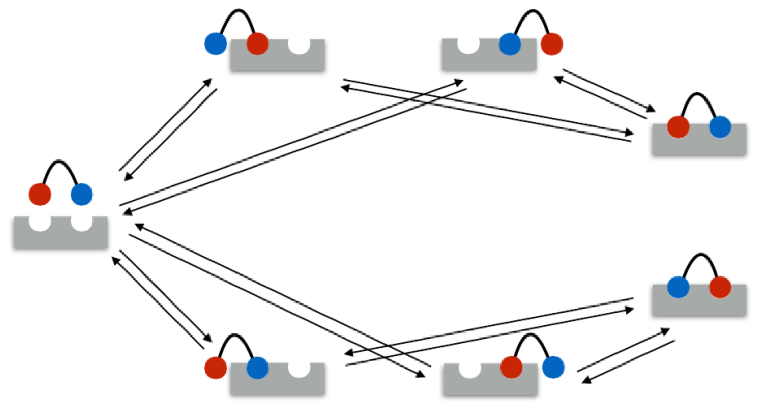
In the following example, the rate matrix is set up for a bivalent system. As mentioned above, in the bivalent case, there are seven different binding states: 1 unbound state, 4 monovalent binding states, and 2 bivalent binding states. These seven states are illustrated in Figure 1. Therefore, the rate matrix is of size $7\times 7$. Assume the ligands 1 and 2 and the receptors A and B.

In the example, the seven states were ordered as listed in

Table 2. Order of the seven possible states for bivalent bindings: as described in Section 2, $\left[L{R}^1\right]$ comprises the sum of the conformational states II, ..., V, and $\left[L{R}^2\right]$ comprises the sum of states VI and VII.

State Number	Combination	Number of Bindings
I	$\left[\begin{array}{c}1-\\ 2-\end{array}\right]$	0
II	$\left[\begin{array}{c}1A\\ 2-\end{array}\right]$	1
III	$\left[\begin{array}{c}1B\\ 2-\end{array}\right]$	1
IV	$\left[\begin{array}{c}1-\\ 2B\end{array}\right]$	1
V	$\left[\begin{array}{c}1-\\ 2A\end{array}\right]$	1
VI	$\left[\begin{array}{c}1A\\ 2B\end{array}\right]$	2
VII	$\left[\begin{array}{c}1B\\ 2A\end{array}\right]$	2

.

Our model considers every possible combination of each ligand interacting with each receptor. In general, the states can also be summarized into $n+1$ states, i.e., one unbound state, one singly-bound state, one doubly-bound state, ..., and one fully-bound state. Then, the rate matrix is of size $(n+1)\times (n+1)$. This is particularly useful for bigger valency numbers n, i.e., decavalent bindings and above. However, in the following, the procedure is explained in detail for all possible states in the bivalent case. The matrix entries depend on the order of the states, the receptor concentration $c_R$, as well as on the two $k_{on}$ and two $k_{\mathrm{off}}$ rates, where $k_{o{n}_1}$ represent the binding rate for the first (monovalent) binding and $k_{o{n}_2}$ the second (bivalent) binding. $k_{{\mathrm{off}}_2}$ represents the first unbinding, i.e., from the bivalent to monovalent state, and $k_{{\mathrm{off}}_1}$ represents the second unbinding rate (from the monovalent to unbound state). The diagonal elements are the sum of the remaining column entries such that the column sum of K is always zero.

Note that the positions of the entries in the submatrix on the upper right diagonal (in the red box):

$$\left[\begin{array}{cc}{k}_{{\mathrm{off}}_2}& 0\\ 0& k_{{\mathrm{off}}_2}\\ k_{{\mathrm{off}}_2}& 0\\ 0& k_{{\mathrm{off}}_2}\end{array}\right]$$

depend on the order of the states. Likewise, this submatrix transpose with the $k_{o{n}_2}$-values instead of $k_{{\mathrm{off}}_2}$ is inserted below the diagonal (see the submatrix in the blue dotted box). The matrix size increases exponentially. The rate matrix for the n-valent binding is only sketched schematically.

$$K=\left(\begin{array}{cccccc}\ast & k_{\mathrm{off}}& 0& 0& \cdots & 0\\ k_{on}·c_L& \ast & X_1& 0& \cdots & 0\\ 0& Y_1& \ast & X_2& \cdots & 0\\ 0& \cdots & \cdots & \ddots & ⋮& 0\\ 0& 0& \cdots & Y_2& \ast & X_{n-1}\\ 0& 0& 0& \cdots & Y_{n-1}& \ast \end{array}\right)$$

Legend:

*	diagonal matrix with the negative column sum such that the column sum is zero
koff	row vector of length $n^2$ with entry $k_{{\mathrm{off}}_1}$
$k_{on}·c_L$	column vector of length $n^2$ with entry $c_L·k_{{on}_1}$
$X_i$	sparse matrix of size $(\left(\genfrac{}{}{0pt}{}{n}{i}\right)·n\times \left(\genfrac{}{}{0pt}{}{n}{i+1}\right)·n)$ with entries $k_{{\mathrm{off}}_2}$ to $k_{{\mathrm{off}}_n}$, respectively.
	The positions of these entries depend on the theoretical order of conformational states.
$Y_i$	sparse matrix of size $(\left(\genfrac{}{}{0pt}{}{n}{i+1}\right)·n\times \left(\genfrac{}{}{0pt}{}{n}{i}\right)·n)$ with entries $k_{o{n}_2}$ to $k_{o{n}_n}$, respectively.
	The positions of the entries are the transpose of the respective $X_i$ submatrices.

Let $\left[I\right],\left[II\right],\dots ,\left[n_{states}\right]$ be the number of molecules in the respective conformation $1,\dots ,n_{states}$. Then, the corresponding ODE system for n-valent bindings to be solved is:

$${\displaystyle \frac{d}{dt}}\left(\begin{array}{c}\left[I\right]\\ \left[II\right]\\ ⋮\\ [n_{states}]\end{array}\right)=\mathbf{K}\left(\begin{array}{c}\left[I\right]\\ \left[II\right]\\ ⋮\\ [n_{states}]\end{array}\right)$$

PCCA+

Our Markov process is space and time continuous and therefore needs to be discretized for numerical results. A possible discretization method is the Galerkin discretization. The key idea is to project this Markov process onto fewer macro states, i.e., in the bivalent case, we project the $7\times 7$ matrix K on a $2\times 2$ matrix in order to cluster these seven states into only two distinct states: bound and unbound. To do so, the robust Perron cluster analysis (PCCA+) algorithm of Röblitz and Weber [23] was used. Therefore, the eigenvalues of K are computed first according to:

$$KX=X\Lambda$$

with X the matrix of all the eigenvectors and a diagonal matrix of eigenvalues $\Lambda =diag({\lambda }_1,\dots ,{\lambda }_{n+1})$. In this case, only two eigenvalues are of interest because all the states will be clustered into two states only. The eigenvector corresponding to the biggest eigenvalue is called the Perron eigenvalue. For rate matrices, the biggest eigenvalue is always $\lambda =0$. This leading eigenvalue and its corresponding leading eigenvector were selected. The second eigenvector has to satisfy the criterion that the first entry and the respective last one have the maximum distance, to make sure that the two states “unbound” and “bound” are as distinct as possible. For regular matrices K, the clustering algorithm gives a membership matrix $\chi$ by:

$$\chi =XA$$

with A being a matrix of linear factors computed by an optimization process within the clustering algorithm. $\chi$ is a $7\times 2$ matrix stating the degree of membership of each of the seven states to the unbound and bound states, respectively. Its row sum is always one. Finally, K is Galerkin discretized weighted by the stationary distribution $\Pi$ into $K_c$ (clustered K) using $\chi$.

$$K_c={({\chi }^T\Pi \chi )}^{-1}{\chi }^T\Pi K\chi$$

Since we project on a two-dimensional subspace, our $K_c$ matrix is of size $2\times 2$ and has the following entries:

$$K_c=\left(\begin{array}{cc}-k_{on}·c_R& k_{\mathrm{off}}\\ k_{on}·c_R& -k_{\mathrm{off}}\end{array}\right)$$

By dividing the lower left matrix entry by the respective receptor concentration $c_R$ of the titration step, we determine the overall binding rate $k_{on}$. This projection is only possible because we project on an invariant subspace. No crucial information is lost by the clustering.

The following Algorithm 1 shows how the PCCA+ clustering is used to determine the optimal $k_{on}$ and $k_{\mathrm{off}}$ values.

Algorithm 1: Find the optimal overall $k_{on}$ curve after clustering

Require: 14 k_on-ITC and cR values from ITC

P ← permutation matrix of possible k_on and k_off values

for all rows of P do

set up rate matrix K;

for all titration steps t do

perform PCCA+ to obtain $Kc$;

k_on $\leftarrow Kc(2,1)/cR\left(t\right)$;

end for

C ← correlation coefficient of k_on-ITC and k_on;

index $\leftarrow max\left(C\right)$;

end for

return P(index), k_on(index);

For details of the PCCA+ algorithm and specific MATLAB code with examples, please consult [35] (specifically the file optimizeMetastab.m in folder “Figure 6”) and the respective paper.

5. Results and Discussion

To test the model fit, the overall binding rate $k_{on}$ was calculated and compared to the observed binding rate $k_{on-ITC}$ from the experiments. Therefore, the input variables for the mathematical model had to be fitted by a sensitivity analysis. The goal was to achieve the same qualitative behavior of the $k_{on-ITC}$ curve over time, that is over the titration steps and our computed $k_{on}$ curve. That means that the slope including anomalies like kinks should be equal. The goodness of fit was assessed via the correlation coefficient for the lower left entry $K_c(2,1)$, divided by the receptor concentration $c_R$ of the respective titration step and the $k_{on}$ from ITC experiments for each time step. The algorithm was tested for the bivalent Man(1,5)-5, trivalent Man(1,3,5)-5, and pentavalent Man(1,3,5,7,9)S-9 binding processes.

The valency of receptor and ligand was not always the same in the experiments. For setting up the rate matrix, one overall valency of the interaction process was needed. Because we assumed a one-to-one stoichiometry, we used the minimum number of binding sites of the receptor and ligand, i.e., $n=min(n_{ligand},n_{receptor})$. As we will see next, the subsequent projection and clustering of the rate matrix mimicked the experimental $k_{on}$ rate behavior very well. By allowing the theoretical $k_{on}$ and $k_{\mathrm{off}}$ rates to move on a logarithmic scale, i.e., from ${10}^0$–${10}^4$, some further conclusions of the valency of the overall binding can be drawn. If the single $k_{on}$ rates were searched for in a limited range due to computation time limits, it is not possible to learn about the different affinities of the binding steps. We were interested in the relation of say the first binding and the second. For instance, a first binding is quite rare, but if it is made, a second binding is 100-times more likely.

The subsequent discussion of the results should be considered as a preliminary explanation of the systematic change of the $k_{on}$ and $k_{\mathrm{off}}$ rates of the kinITC experiments. Actually, kinITC is a suitable tool for describing: $L+R\begin{array}{c}\underrightarrow{k_{on}}\\ \overleftarrow{k_{\mathrm{off}}}\end{array}LR$ settings, but for higher valent bindings, a mathematical projection becomes necessary. For the following comparison, the first 14 titration steps of each experiment were considered (see the Supplementary Information (SI) for experimental data).

5.1. Bivalent Model Fitting

Man(1,5)-5

The experimental and computed $k_{on}$ rates are depicted in Figure 2. The correlation coefficient was 0.98. The experimental $k_{on}$ showed a clear upward slope. To interpret these binding and unbinding rates from a mathematical model point of view, this constellation seemed to be a monovalent binding process, as only the first binding rate $k_{o{n}_1}=100$ was high, while the second one $k_{o{n}_2}=1$ was very low. Both unbinding rates were very low, $k_{{\mathrm{off}}_1}=1$ and $k_{{\mathrm{off}}_2}=1$. We can assume that unbinding was very unlikely. All in all, there seemed to be one binding taking place, which was the equilibrium.

5.2. Trivalent Model Fitting

Man(1,3,5)-5

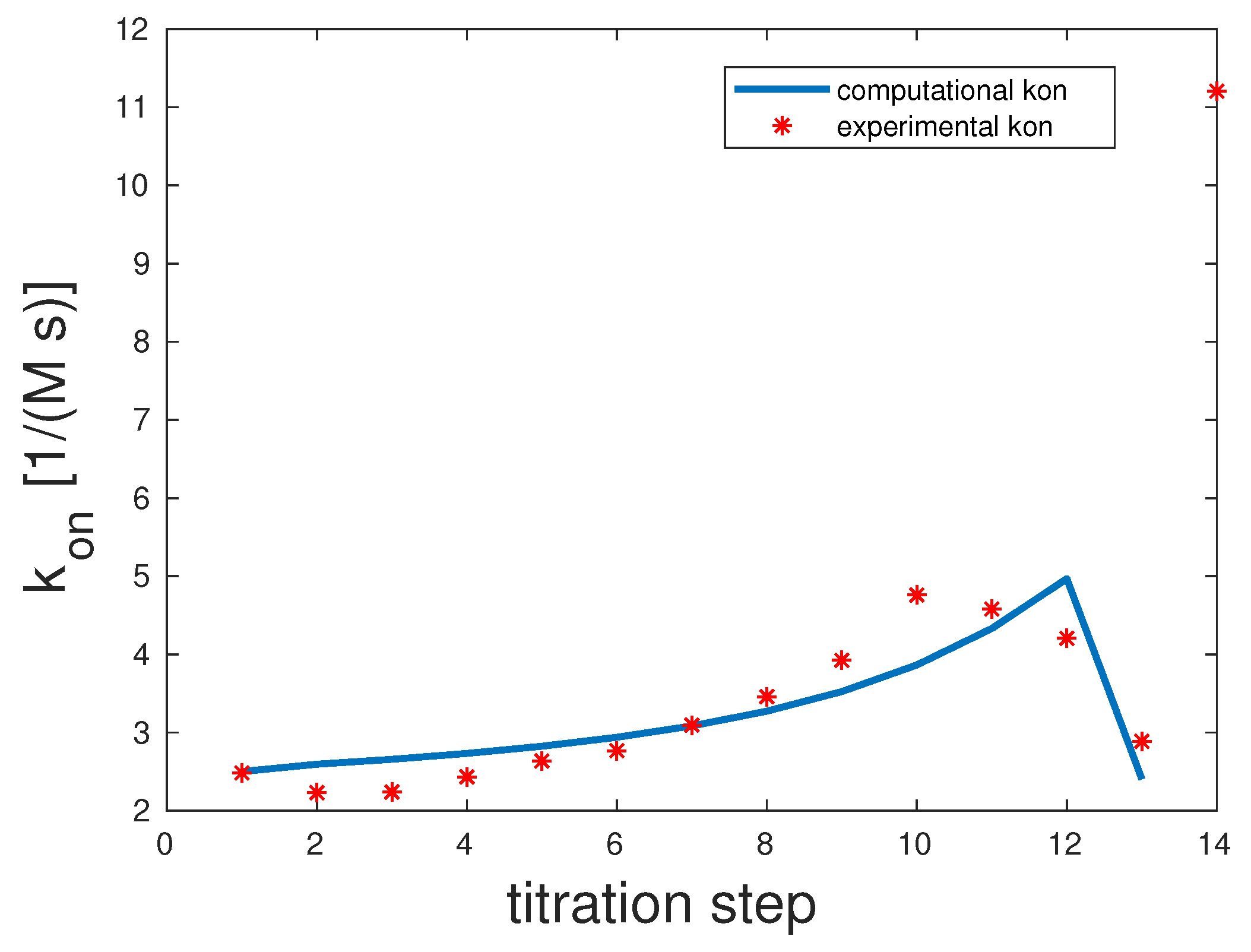
As shown in Figure 3, only 13 out of 14 titration steps were considered for the fitting procedure. The 14^th overall $k_{on}$ value was clearly an outlier, probably due to measurement inconsistencies. For completeness, it is depicted in the graph. The correlation coefficient was 0.87. The binding rates were the following: $k_{o{n}_1}=1000,k_{o{n}_2}=1000,k_{o{n}_3}=1000$. All three unbinding rates were $k_{{\mathrm{off}}_i}=1$. One possible interpretation is that all the fully-bound state was what Whitesides called the kinetic origin of high stability [36].

5.3. Pentavalent Model Fitting

Man(1,3,5,7,9)S-9

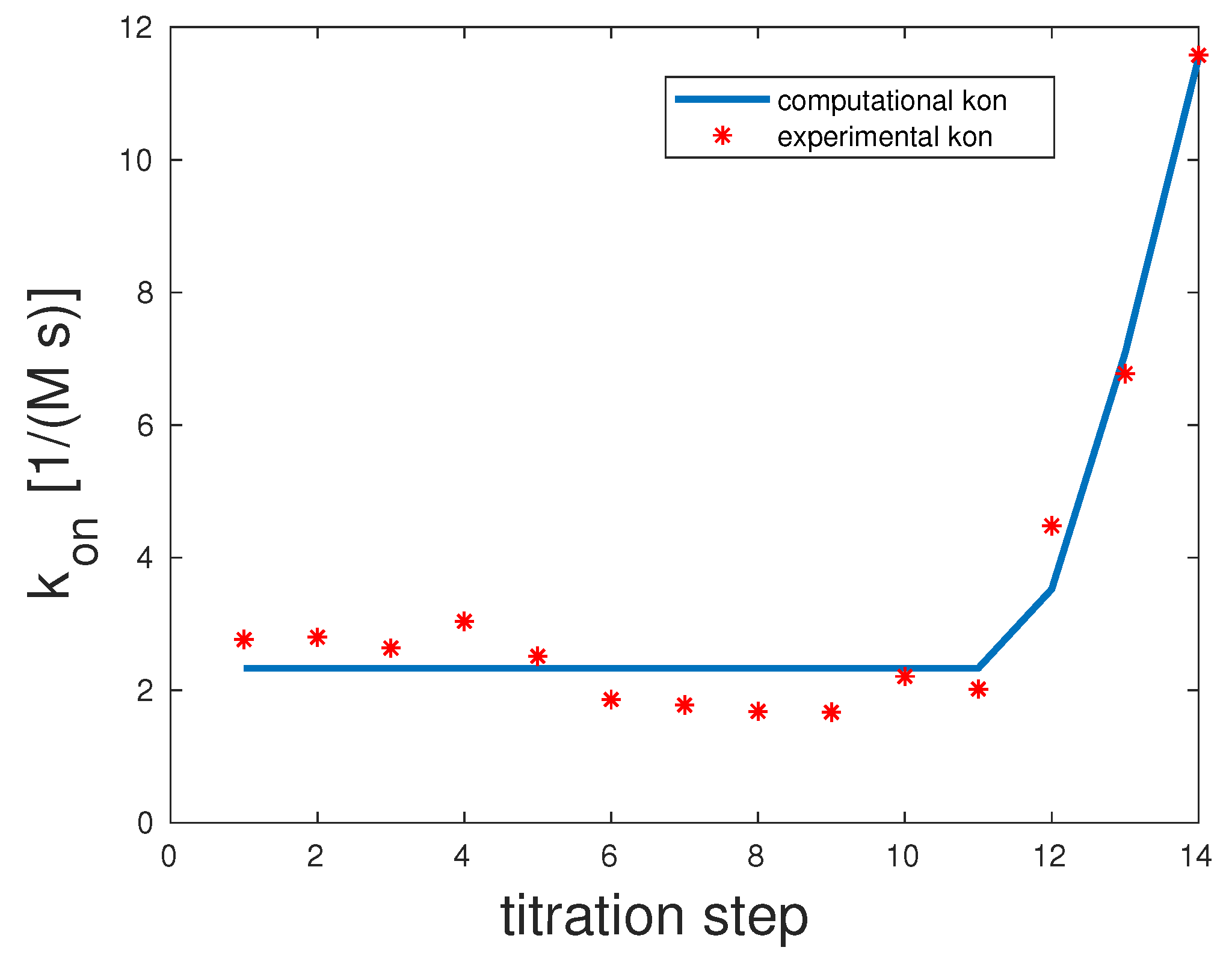
In the pentavalent example, there were only four specific $k_{on}$ and $k_{\mathrm{off}}$ rates and not five. This was due to the fact that Con A was tetrameric, and within the model when assuming a one-to-one stoichiometry, there can only be a maximum of min $(n_{ligands},n_{receptor})=min(4,5)=4$ single bonds. Experimental and computed $k_{on}$ rates are illustrated in Figure 4.

The correlation coefficient for this example was 0.98. The scenario representing the best fit for this model showed that the first and second binding seemed to be highly unlikely with $k_{o{n}_1}=k_{o{n}_2}=1$, but once they took place, the third binding happened almost surely with $k_{o{n}_3}=$ 10,000. The last binding was again unlikely with $k_{o{n}_4}=10$. $k_{{\mathrm{off}}_1}=$ 10,000 and $k_{{\mathrm{off}}_2}=k_{{\mathrm{off}}_3}=k_{{\mathrm{off}}_4}=1$. That means that overall unbinding was very low if there was more than one binding. If there was only one bond between the mannose and Con A, dissociation was very likely.

5.4. Limitations of the Model and Discussion

The deviation of the modeled $k_{on}$ rates to the experimental ones was due to several reasons. Our mathematical model was a simplification of complex binding processes and therefore had theoretical limitations. First, our mathematical models assumed a one-to-one stoichiometry. So far, intermolecular complex formation has been neglected. Especially for ligands with many binding sites, this intermolecular crosslinking does occur. This phenomenon was not considered in our mathematical model and can partly explain the deviations from our computed $k_{on}$ rates to the experimental rates $k_{on-ITC}$. Secondly, so far, no rebinding has been considered. Every binding was treated as a first time ligand–receptor interaction no matter if this very couple was bound before. The heat absorption due to unbinding was not yet taken into account, but very likely had an effect on the ITC signal. As discussed in the outlook, we are working on a rebinding quantification for a better interpretation of the kinITC results.

Third, we solved an inverse problem by fitting four (two $k_{on}$ rates and two $k_{\mathrm{off}}$ rates in the bivalent case), six (three $k_{on}$ rates and three $k_{\mathrm{off}}$ rates in the trivalent case), or eight (four $k_{on}$ rates and four $k_{\mathrm{off}}$ rates in the pentavalent case) specific binding and unbinding rates knowing 14 different titration data. We do not claim that our solution found was the only possible interpretation of the laboratory data with regard to our model. There may be other combinations that will yield a comparably good fit. For instance, in the trivalent example, 15,625 different combinations ($5^6$ because five different values for each of the three $k_{on}$ and $k_{\mathrm{off}}$) of the $k_{on}$ and $k_{\mathrm{off}}$ rates were considered. Out of these, 25 had the maximum correlation coefficient. The results shown in this paper are one example out of these 25 fits. Despite not delivering unique results, this method helped in excluding inappropriate models.

The ITC method can be fragile, and single outliers occur due to experimental limitations. The thermodynamic parameters of the ITC data can have errors stemming from the ligand and receptor concentrations, unfavorable fitting procedures, and baseline drift. Other error sources were a combination of random noise, unclear instrument response time, uncertainty in $K_a$, and the instrumental rate constant $k_{ITC}$ [16]. For an uncertainty quantification in the experimental data used in the practical part, see Igde et al. [14]. Numerically, the $k_{on}$ parameters from our computation do not correspond to the kinITC experimental data yet. However, it is possible to model such a complicated process showing the same qualitative behavior with each titration step. Shifting our computed $k_{on}$ rates down to the experimental $k_{on-ITC}$ baseline level allowed for slope comparison. This is due to the fact that the $k_{o{n}_i}$ and $k_{{\mathrm{off}}_i}$ parameters were assumed to be on an exponential scale. This scaling could be refined further or even made adaptive to tackle this problem.

6. Conclusions and Outlook

This paper demonstrated that the overall binding rate of a ligand–receptor interaction implies a systematic dependency of the $k_{on}$ rates with regard to the titration steps. Taking the average $k_{on}$ value over all titration steps did not fully account for the whole process. It is possible to compute the overall binding rate of multivalent bindings, only by knowing the valency number and the ligand concentration per titration step. Our subspace projection approach could be successfully applied to kinITC data. The key finding of this study is that we can learn about the system’s association rate by projecting a high-dimensional process on a two-dimensional space, namely bound and unbound. Doing so, we obtained a binding rate $k_{on}$ per time step, i.e., one for each titration step. This rate showed the same qualitative behavior as the overall $k_{on}$ rate obtained from the kinITC experiments. This finding will be useful for the prediction of the binding behavior when no experimental data, but only the ligand and receptor concentration, are available.

Our method still has some limitations. In the present model, we assumed one-to-one bindings between ligands and receptors. However, other stoichiometries such as intermolecular aggregations were possible and could occur in the experiments. If this was not possible, an error estimate for overall $k_{on}$ rates would be necessary, as they were the result of a slightly different stoichiometric model.

Another aspect that was not considered in this paper is the so-called rebinding effect where the probability of a monovalent binding event of multivalent ligands is increased by the high local concentration of ligands with no regard to potential multivalent receptor binding. So far, there has been no distinction made between rebinding and new binding. Mathematically, there already existed a quantification of the lower bound of rebinding in the system [32,37]. Such an estimation could also be applied numerically for ITC data as presented in this paper.

References

- Lundquist, J.J.; Toone, E.J. The cluster glycoside effect. Chem. Rev. 2002, 102, 555–578. [Google Scholar] [CrossRef] [PubMed]
- Mammen, M.; Choi, S.K.; Whitesides, G.M. Polyvalent interactions in biological systems: Implications for design and use of multivalent ligands and inhibitors. Angew. Chem. Int. Ed. 1998, 37, 2754–2794. [Google Scholar] [CrossRef]
- Cairo, C.W.; Gestwicki, J.E.; Kanai, M.; Kiessling, L.L. Control of multivalent interactions by binding epitope density. J. Am. Chem. Soc. 2002, 124, 1615–1619. [Google Scholar] [CrossRef] [PubMed]
- Gestwicki, J.E.; Cairo, C.W.; Strong, L.E.; Oetjen, K.A.; Kiessling, L.L. Influencing receptor- ligand binding mechanisms with multivalent ligand architecture. J. Am. Chem. Soc. 2002, 124, 14922–14933. [Google Scholar] [CrossRef] [PubMed]
- Hunter, C.A.; Tomas, S. Cooperativity, partially bound states, and enthalpy-entropy compensation. Chem. Biol. 2003, 10, 1023–1032. [Google Scholar] [CrossRef] [PubMed]
- Hunter, C.A.; Anderson, H.L. What is cooperativity? Angew. Chem. Int. Ed. 2009, 48, 7488–7499. [Google Scholar] [CrossRef] [PubMed]
- Kiessling, L.L.; Pohl, N.L. Strength in numbers: Non-natural polyvalent carbohydrate derivatives. Chem. Biol. 1996, 3, 71–77. [Google Scholar] [CrossRef]
- Fasting, C.; Schalley, C.A.; Weber, M.; Seitz, O.; Hecht, S.; Koksch, B.; Dernedde, J.; Graf, C.; Knapp, E.W.; Haag, R. Multivalency as a chemical organization and action principle. Angew. Chem. Int. Ed. 2012, 51, 10472–10498. [Google Scholar] [CrossRef]
- Ercolani, G.; Schiaffino, L. Allosteric, chelate, and interannular cooperativity: A mise au point. Angew. Chem. Int. Ed. 2011, 50, 1762–1768. [Google Scholar] [CrossRef]
- Ambrosi, M.; Cameron, N.R.; Davis, B.G. Lectins: Tools for the molecular understanding of the glycocode. Org. Biomol. Chem. 2005, 3, 1593–1608. [Google Scholar] [CrossRef]
- Brewer, C.F.; Miceli, M.C.; Baum, L.G. Clusters, bundles, arrays and lattices: Novel mechanisms for lectin–saccharide-mediated cellular interactions. Curr. Opin. Struct. Biol. 2002, 12, 616–623. [Google Scholar] [CrossRef]
- Ambrosi, M.; Cameron, N.R.; Davis, B.G.; Stolnik, S. Investigation of the interaction between peanut agglutinin and synthetic glycopolymeric multivalent ligands. Org. Biomol. Chem. 2005, 3, 1476–1480. [Google Scholar] [CrossRef] [PubMed]
- Müller, C.; Despras, G.; Lindhorst, T.K. Organizing multivalency in carbohydrate recognition. Chem. Soc. Rev. 2016, 45, 3275–3302. [Google Scholar] [CrossRef] [PubMed] [Green Version]
- Igde, S.; Röblitz, S.; Müller, A.; Kolbe, K.; Boden, S.; Fessele, C.; Lindhorst, T.K.; Weber, M.; Hartmann, L. Linear Precision Glycomacromolecules with Varying Interligand Spacing and Linker Functionalities Binding to Concanavalin A and the Bacterial Lectin FimH. Macromol. Biosci. 2017, 17, 1700198. [Google Scholar] [CrossRef] [PubMed]
- Burnouf, D.; Ennifar, E.; Guedich, S.; Puffer, B.; Hoffmann, G.; Bec, G.; Disdier, F.; Baltzinger, M.; Dumas, P. kinITC: A new method for obtaining joint thermodynamic and kinetic data by isothermal titration calorimetry. J. Am. Chem. Soc. 2011, 134, 559–565. [Google Scholar] [CrossRef] [PubMed]
- Vander Meulen, K.A.; Butcher, S.E. Characterization of the kinetic and thermodynamic landscape of RNA folding using a novel application of isothermal titration calorimetry. Nucleic Acids Res. 2011, 40, 2140–2151. [Google Scholar] [CrossRef] [PubMed] [Green Version]
- Freire, E.; Mayorga, O.L.; Straume, M. Isothermal titration calorimetry. Anal. Chem. 1990, 62, 950A–959A. [Google Scholar] [CrossRef]
- Pierce, M.M.; Raman, C.; Nall, B.T. Isothermal titration calorimetry of protein–protein interactions. Methods 1999, 19, 213–221. [Google Scholar] [CrossRef]
- Leavitt, S.; Freire, E. Direct measurement of protein binding energetics by isothermal titration calorimetry. Curr. Opin. Struct. Biol. 2001, 11, 560–566. [Google Scholar] [CrossRef]
- Dumas, P.; Ennifar, E.; Da Veiga, C.; Bec, G.; Palau, W.; Di Primo, C.; Piñeiro, A.; Sabin, J.; Muñoz, E.; Rial, J. Extending ITC to Kinetics with kinITC. In Methods in Enzymology; Elsevier: Amsterdam, The Netherlands, 2016; Volume 567, pp. 157–180. [Google Scholar]
- Åberg, C.; Duderstadt, K.E.; van Oijen, A.M. Stability versus exchange: A paradox in DNA replication. Nucleic Acids Res. 2016, 44, 4846–4854. [Google Scholar] [CrossRef]
- Deuflhard, P.; Weber, M. Robust Perron cluster analysis in conformation dynamics. Linear Algebra Appl. 2005, 398, 161–184. [Google Scholar] [CrossRef] [Green Version]
- Röblitz, S.; Weber, M. Fuzzy spectral clustering by PCCA+: Application to Markov state models and data classification. Adv. Data Anal. Classif. 2013, 7, 147–179. [Google Scholar] [CrossRef]
- Weber, M.; Fackeldey, K. G-pcca: Spectral Clustering for Non-Reversible Markov Chains; ZIB-Report; Konrad-Zuse-Zentrum für Informationstechnik Berlin: Berlin, Germany, 2015; pp. 15–35. [Google Scholar]
- Kugel, J.A.; Goodrich, J.F. Binding and Kinetics for Molecular Biologists; CSHL Press: The Cold Spring Harbor, NY, USA, 2007; Volume 127. [Google Scholar]
- Keller, S.; Vargas, C.; Zhao, H.; Piszczek, G.; Brautigam, C.A.; Schuck, P. High-precision isothermal titration calorimetry with automated peak-shape analysis. Anal. Chem. 2012, 84, 5066–5073. [Google Scholar] [CrossRef] [PubMed]
- Praefcke, G.J.; Herrmann, C. Isotherme Titrationskalorimetrie (ITC) zur Charakterisierung biomolekularer Wechselwirkungen. BIOspektrum 2005, 1, 44–47. [Google Scholar]
- Egawa, T.; Tsuneshige, A.; Suematsu, M.; Yonetani, T. Method for determination of association and dissociation rate constants of reversible bimolecular reactions by isothermal titration calorimeters. Anal. Chem. 2007, 79, 2972–2978. [Google Scholar] [CrossRef]
- Dumas, P. KinITC—Affinimeter Blog. 2018. Available online: https://www.affinimeter.com/site/kinitc-2/ (accessed on 20 June 2019).
- Igde, S. Assessing the Influence of Different Structural Features on Multivalent Thermodynamics and Kinetics of Precision Glycomacromolecules. Ph.D. Thesis, Freie Universität Berlin, Berlin, Germany, 2016. [Google Scholar]
- Nowak, U.; Weimann, L. Numerical Solution of Nonlinear (NL) Least Squares (S) Problems with Nonlinear Constraints (CON), Especially Designed for Numerically Sensitive Problems. 2017. Available online: http://elib.zib.de/pub/elib/codelib/nlscon_m/nlscon.m (accessed on 10 July 2019).
- Röhl, S.; Weber, M.; Fackeldey, K. Computing the minimal rebinding effect for nonreversible processes. 2018. Submitted for publication. [Google Scholar]
- Syski, R. Passage Times for Markov Chains; Ios Press: Tepper Drive Clifton, VA, USA, 1992; Volume 1. [Google Scholar]
- Berberan-Santos, M.; Martinho, J. The integration of kinetic rate equations by matrix methods. J. Chem. Educ. 1990, 67, 375. [Google Scholar] [CrossRef]
- Weber, M. Matlab-software and data sets to recapitulate the presented results. Implications of PCCA+ in Molecular Simulation. Computation 2018, 6, 20. [Google Scholar] [CrossRef]
- Rao, J.; Lahiri, J.; Weis, R.M.; Whitesides, G.M. Design, synthesis, and characterization of a high-affinity trivalent system derived from vancomycin and L-Lys-D-Ala-D-Ala. J. Am. Chem. Soc. 2000, 122, 2698–2710. [Google Scholar] [CrossRef]
- Weber, M.; Fackeldey, K. Computing the minimal rebinding effect included in a given kinetics. Multiscale Model. Simul. 2014, 12, 318–334. [Google Scholar] [CrossRef]
Figure 1.
Bivalent bindings have seven possible states. The ligand binding sites are equal. The red and blue color refer to the possible binding permutations.
Figure 2.
Comparison of the computed and experimental [14] rates for bivalent Man(1,5)-5; see the Supplementary Information (SI) for additional information on experimental data. The theoretical rates were 100 and one, and those of were one and one.
Figure 3.
Comparison of the computed and experimental [14] rates for bivalent Man(1,3,5)-5. The rates were 1000, 1000, and 1000 and for were 1, 1, and 1.
Figure 4.
Comparison of the computed and experimental [14] rates for pentavalent Man(1,3,5,7,9)S-9; see the Supplementary Information (SI) for additional information on experimental data. The rates were 1, 1, 10,000, and 10 and for were 10,000, 1, 1, and 1.