Implementation and Validation of Semi-Implicit WENO Schemes Using OpenFOAM^®

Abstract

In this article, the development of high-order semi-implicit interpolation schemes for convection terms on unstructured grids is presented. It is based on weighted essentially non-oscillatory (WENO) reconstructions which can be applied to the evaluation of any field in finite volumes using its known cell-averaged values. Here, the algorithm handles convex cells in arbitrary three-dimensional meshes. The implementation is parallelized using the Message Passing Interface. All schemes are embedded in the code structure of OpenFOAM^® resulting in the access to a huge open-source community and the applicability to high-level programming. Several verification cases and applications of the scalar advection equation and the incompressible Navier-Stokes equations show the improved accuracy of the WENO approach due to a mapping of the stencil to a reference space without scaling effects. An efficiency analysis indicates an increased computational effort of high-order schemes in comparison to available high-resolution methods. However, the reconstruction time can be efficiently decreased when more processors are used.

1. Introduction

In recent years, open source Computational Fluid Dynamics (CFD) codes experienced an increased influence not only on ongoing science but also on the industry. It is caused by providing a suitable environment for a wide range of new developments as well as different solvers for multiple applications at no charge. Among others, the Finite Volume Method (FVM)-based open source C++ library OpenFOAM^® gained popularity in the recent past since it can handle unstructured grids with polyhedral cells and provides a high-level programming platform for applying new solvers easily. Unstructured meshes are currently in the focus of operators due to their increased versatility in the application CFD methods in complex geometries [1] and the reduced generation time. However, the irregular structure of the grid prevents most codes such as OpenFOAM^® to reach more than second order of accuracy. Further, the commonly applied second-order methods such as total variation diminishing (TVD) schemes are derived for structured grids. This might cause unbounded solutions on unstructured grids dependent on the chosen gradient scheme.

High-order methods would be preferable especially for the challenging task of discretising convective terms. Related to turbulence flows, high-order methods increase the accuracy of simulating mixing by reducing numerical diffusion significantly. At the same time, convection dominant flows, resulting in an appearance of hyperbolic aspects in the underlying equations, require monotonic schemes to assure stability [2]. Such challenging tasks arise e.g., in flows with discontinuities such as shocks or free surfaces. A suitable scheme has to be chosen which copes with the formation of large gradients in front propagating problems and preserve the sharpness of the interface without creating spurious oscillations near discontinuities at the interface [3]. This Gibbs-like phenomenon generates $\mathcal{O}\left(1\right)$ spurious oscillations at points of discontinuity, proportional to the size of the jump [4].

Linear schemes with such monotone behaviour are restricted to first-order accuracy according to Godunov [5]. Therefore, non-linear schemes were developed such as TVD schemes which are based on limiters derived from corresponding conditions of Sweby [6]. Their main drawbacks are the degeneration to first-order accuracy near extrema regardless of a smooth peak or discontinuity and at most second-order accuracy. This led to the development of (weighted) essentially non-oscillatory ((W)ENO) schemes. They introduce non-linear weighting for preventing oscillations near discontinuities and simultaneously reach an arbitrary order of accuracy in smooth regions. However, the solution is not strictly bounded leading to the eventual necessity of additional limiting [7].

The first ENO scheme based on adaptive stencils was developed by Harten et al. [4]. Their scheme searches for the most suitable cells in a dynamic manner in order to obtain a stencil with the smoothest solution in each time step. The application on unstructured grids was provided by Abgrall [8] for the first time. The drawbacks of ENO methods are the prevention of convergence in the case of frequent switching of the stencil from one time step to another and costly operations at runtime reducing the overall performance [9]. An alternative scheme, named Quasi-ENO, was introduced by Ollivier-Gooch [9] to overcome these drawbacks. In contrast to classical ENO schemes, it is based on a high-order least-squares reconstruction which fulfils the ENO-property by a pointwise data-dependent weighting in one fixed, central stencil [10]. Classical least-squares reconstructions are able to reach high-orders in smooth regions but fail near discontinuities. A common way of eliminating this problem is introducing a limiter as Wang [11] and McDonald [12] demonstrated. However, the underlying mathematical problem is the inclusion of the data from cells behind a discontinuity into the reconstruction. The Quasi-ENO scheme solves this problem in a more efficient way than the classical ENO scheme and furthermore, offers the possibility of excluding cells of poor quality from the reconstruction. It has been shown by the authors [13] that the Quasi-ENO approach provides accurate solutions as long as the topology allows compact stencils without scaling effects. However, the solutions of the systems of equations often have to be calculated from ill-conditioned matrices, particularly in case of higher order polynomials. The common way of improving the condition numbers by applying preconditioning fails for the ENO weighted reconstruction matrices. Further, the stencils may lose too much information for reaching the nominal order of accuracy near discontinuities which results in a reduction of the order similar to TVD schemes [14].

In contrast to ENO, WENO schemes compute the solution on several fixed stencils and combine them by a non-linear weighting in order to obtain a final smooth solution. The weights are calculated from an evaluation of the smoothness in each stencil. This theoretically leads up to $(2r+1)$th order of accuracy by using a polynomial of rth-order [10]. Further, they yield better convergence due to smoother numerical fluxes [15]. In return, they need the preparation of several stencils which is computationally quite expensive in preprocessing especially on unstructured meshes in three dimensions [16]. Besides, the reconstruction may fail near critical points, on very coarse grids or if not enough smooth data is provided [17]. The first WENO scheme was introduced by Liu et al. [18] and Jiang and Shu [19] on regular grids. Later, Friedrich [20] extended it to two-dimensional, unstructured grids. In the recent past, Dumbser and Käser [16] and Tsoutsanis et al. [1] accomplished that finite volume WENO schemes are applicable on three-dimensional, unstructured grids with arbitrary order of accuracy. Pringuey [3] successfully extended their approach to non-uniform cells and sketched the possibility to implement WENO schemes in OpenFOAM^®. However, in his work, he restricted the usage to explicit convection terms in hyperbolic equations and provided less information about the implementation into the code itself.

The presented research, therefore, aims firstly at a derivation and detailed verification of a WENO reconstruction method fully embedded in the existing code structure of OpenFOAM^® using a similar approach to [3]. This provides high-order reconstructions on unstructured grids to a huge group of researchers and enables these developments to a broad scope of applications for the first time. The method is mainly based on the approach of Dumbser and Käser [16] and Tsoutsanis et al. [1]. Hence, the scheme operates in a reference space without scaling effects in order to prevent ill-conditioned matrices and improve the accuracy on irregular grids. All mesh types are handled automatically which is in accordance to OpenFOAM^®. On these general grids, finite volume WENO schemes were usually applied to convection terms in an explicit manner. As an exceptional example, implicit discontinuous Galerkin methods based on hierarchical WENO reconstructions might be of interest to the reader [21]. The possibility to build a semi-implicit finite volume WENO convection scheme arises by including the reconstruction in OpenFOAM^® due to existing code structures for such an implementation. It results in a more stable reconstruction for larger time steps and an utilization of high-order convection schemes in common semi-implicit solution algorithms such as SIMPLE or PISO (Pressure-Implicit with Splitting of Operators). However, the theoretical accuracy limitation of these algorithms can of course not be affected.

In Section 2, the derivation of the basic reconstruction method is presented. Here, especially the parallelisation process within the 0-halo approach of OpenFOAM^® is described in detail. Afterwards, the derivations of semi-implicit WENO convection schemes (Section 3) and different gradient schemes (Section 4) are given. It follows Section 5 with implementation and application details. Section 6 is dedicated to the verification process of the schemes, whereas Section 7 shows several test cases including an efficiency comparison. A conclusion completes this article in Section 8.

2. Numerical Approach of WENO Reconstruction Methods

The spatial domain is taken in its discretised form of N cells with the volumes $\left|V_i\right|,i=1,\dots ,N$, and the data of any scalar variable $\Phi$ is stored in the cell centres ${\overrightarrow{x}}_i$ represented by the cell averaged values ${\overline{\Phi }}_i$. In case of a vector or tensor field, each component is evaluated separately because of the later introduced weighting. With the aid of a least-squares reconstruction, $\Phi$ is replaced by a polynomial representation $p_i$ in each cell $V_i$ with the constraint of conservation of the mean value within $V_i$. Scaling effects are prevented by mapping the reconstruction process from the physical space $\overrightarrow{x}=\overrightarrow{x}(x,y,z)$ into a reference space $\overrightarrow{\xi }=\overrightarrow{\xi }(\xi ,\eta ,\zeta )$ using an affine transformation $\overrightarrow{x}=\overrightarrow{x}(\xi ,\eta ,\zeta )$ and its inversion $\overrightarrow{\xi }=\overrightarrow{\xi }(x,y,z)$, respectively. The affinity of the transformation conserves the conservation condition which results in

$$\begin{array}{cc}\hfill {\overline{\Phi }}_i& ={\displaystyle \frac{1}{\left|V_i\right|}}{\int }_{V_i}\Phi (\overrightarrow{x})\mathrm{d}x\mathrm{d}y\mathrm{d}z={\displaystyle \frac{1}{\left|V_i^{\prime }\right|}}{\int }_{V_i^{\prime }}\Phi (\overrightarrow{\xi })\mathrm{d}\xi \mathrm{d}\eta \mathrm{d}\zeta ={\displaystyle \frac{1}{\left|V_i^{\prime }\right|}}{\int }_{V_i^{\prime }}{p}_i(\overrightarrow{\xi })\mathrm{d}\xi \mathrm{d}\eta \mathrm{d}\zeta ,\hfill \end{array}$$

(1)

with $V_i^{\prime }$ the mapped cell $V_i$ in its reference space. The polynomials $p_i$ are expressed by an expansion over local polynomial basis functions ${\Omega }_k$ [1]

$$\begin{array}{cc}\hfill p_i(\overrightarrow{\xi })& ={\overline{\Phi }}_i+\sum _{k=1}^K{a}_k{\Omega }_k(\overrightarrow{\xi }).\hfill \end{array}$$

(2)

The number of degrees of freedom K relates to the order of the polynomial r in three dimensions according to

$$\begin{array}{cc}\hfill K& ={\displaystyle \frac{(r+1)(r+2)(r+3)}{6}}-1,\hfill \end{array}$$

(3)

respectively in two dimensions to

$$\begin{array}{cc}\hfill K& ={\displaystyle \frac{(r+1)(r+2)}{2}}-1.\hfill \end{array}$$

(4)

The basis functions ${\Omega }_k$ have to be chosen with the constraint of satisfying (1), equivalent to a zero mean value over $V_i^{\prime }$. The condition can be satisfied analytically by an appropriate definition of the basis functions

$$\begin{array}{cc}\hfill {\Omega }_k(\overrightarrow{\xi })& ={\Psi }_k(\overrightarrow{\xi })-{\displaystyle \frac{1}{\left|V_i^{\prime }\right|}}{\int }_{V_i^{\prime }}{\psi }_k(\overrightarrow{\xi })\mathrm{d}\xi \mathrm{d}\eta \mathrm{d}\zeta ,k=1,\dots ,K,\hfill \end{array}$$

(5)

with arbitrary orthogonal polynomial basis functions ${\Psi }_k$. In accordance with Ollivier-Gooch [9] and Friedrich [20], a Taylor series expansion around the centre of $V_i$ is applied and defined as

$$\begin{array}{cc}\hfill {\Psi }_k(\overrightarrow{\xi })& ={(\xi -{\xi }_i)}^n{(\eta -{\eta }_i)}^m{(\zeta -{\zeta }_i)}^o,\hfill \end{array}$$

(6)

where k corresponds to one combination of $n,m,o$ such that $0\le n+m+o\le r$.

The degrees of freedom $a_k$ are evaluated on a set of stencils $S_m,m=0,\dots ,N_{Si},$ for each cell $V_i$ in comparison to the single, central stencil of classical least-squares reconstructions. By definition, the stencil $S_0$ is the central stencil. The number of sector stencils $N_{Si}$ depends on the cell shape and its closeness to boundaries. For each $S_m$, appropriate neighbouring cells $V_j^{\prime },j=0,\dots ,J_{max}$ in the reference space of $V_i^{\prime }$ are collected. The necessary number if cells $J_{max}$ is an important parameter which is discussed in Section 2.1. By definition, $j=0$ corresponds to the target cell $V_i^{\prime }$. A polynomial $p_m(\overrightarrow{\xi })$ is formulated for each $S_m$ using (2). Afterwards, the WENO reconstructed polynomial of each cell is obtained by a non-linear combination of several $p_m$ according to [16]

$$\begin{array}{cc}\hfill p_{weno,i}(\overrightarrow{\xi })& =\sum _{m=0}^{N_{Si}}{\omega }_m{p}_m(\overrightarrow{\xi }),\hfill \end{array}$$

(7)

with the non-linear weights

$$\begin{array}{cc}\hfill {\omega }_m& ={\displaystyle \frac{{\gamma }_m}{{\sum }_{m=0}^{N_{Si}}{\gamma }_m}},\hfill \end{array}$$

(8)

and ${\gamma }_m$ defined as

$$\begin{array}{cc}\hfill {\gamma }_m& ={\displaystyle \frac{d_m}{{\left(\epsilon +{\mathcal{I}}_{S,m}\right)}^p}},\hfill \end{array}$$

(9)

with $\epsilon ={10}^{-6}$ to prevent the denominator from becoming zero and $p=4$ as discussed in [22]. The linear weights $d_m$ are defined as ${10}^3$ for $d_0$ and 1 else in accordance with Dumbser and Käser [16]. The weights (8) have to determine to what extend the solution in a stencil provides a qualitative contribution to a smooth solution of the polynomial reconstruction in the target cell. Here, the key element is the smoothness indicator ${\mathcal{I}}_{S,m}$, which represents the smoothness indicator of the solution in the stencil $S_m$. It diminishes in case of smooth solutions and, thus, the corresponding weight ${\omega }_m$ increases. The matrix expression for ${\mathcal{I}}_{S,m}$ is given by [3]

$$\begin{array}{cc}\hfill {\mathcal{I}}_{S,m}& =\sum _{s=1}^K{a}_s^{\left(m\right)}·\left(\sum _{t=1}^K{\mathcal{B}}_{st}{a}_t^{\left(m\right)}\right),\hfill \end{array}$$

(10)

where ${\mathcal{B}}_{st}$ is an element of the mesh-independent oscillation indicator matrix $\mathcal{B}$. The aim of the indicator is the minimization of the total variation of the sum of the ${\mathcal{L}}_2$-norms of all derivatives of the polynomial, which is comparable to the TVD property of other convection schemes [19]. This property has to be satisfied by $\mathcal{B}$ which is, therefore, defined as

$$\begin{array}{cc}\hfill {\mathcal{B}}_{st}=\sum _{\lambda =1}^r\sum _{\alpha =0}^{\lambda }\sum _{\beta =0}^{\lambda -\alpha }{\int }_{V_i^{\prime }}& {\displaystyle \frac{{\partial }^{\lambda }}{\partial {\xi }^{\alpha }\partial {\eta }^{\beta }\partial {\zeta }^{\gamma }}}{\Omega }_s(\overrightarrow{\xi })·{\displaystyle \frac{{\partial }^{\lambda }}{\partial {\xi }^{\alpha }\partial {\eta }^{\beta }\partial {\zeta }^{\gamma }}}{\Omega }_t(\overrightarrow{\xi })\mathrm{d}\xi \mathrm{d}\eta \mathrm{d}\zeta ,\hfill \end{array}$$

(11)

with $\gamma =\lambda -\alpha -\beta$ and r the polynomial order. As can be seen from (11), the matrix is solution independent and may be precomputed. Additionally, it is mesh independent through the calculation in the reference space. Under consideration of the definitions for the basis Function (5), Equation (11) can be further simplified to

$$\begin{array}{cc}\hfill {\mathcal{B}}_{st}=\sum _{\lambda =1}^r\sum _{\alpha =0}^{\lambda }\sum _{\beta =0}^{\lambda -\alpha }{\int }_{V_i^{\prime }}& {\displaystyle \frac{{\partial }^{\lambda }}{\partial {\xi }^{\alpha }\partial {\eta }^{\beta }\partial {\zeta }^{\gamma }}}{\Psi }_s(\overrightarrow{\xi })·{\displaystyle \frac{{\partial }^{\lambda }}{\partial {\xi }^{\alpha }\partial {\eta }^{\beta }\partial {\zeta }^{\gamma }}}{\Psi }_t(\overrightarrow{\xi })\mathrm{d}\xi \mathrm{d}\eta \mathrm{d}\zeta .\hfill \end{array}$$

(12)

The monomials are expressed by their orthogonal basis functions as

$$\begin{array}{cc}\hfill {\Psi }_{s,t}(\overrightarrow{\xi })& ={(\xi -{\xi }_i)}^{A_{1,2}}{(\eta -{\eta }_i)}^{B_{1,2}}{(\zeta -{\zeta }_i)}^{C_{1,2}},\hfill \end{array}$$

(13)

with the condition $(A_1,B_1,C_1,A_2,B_2,C_2)\in {[0,r]}^6$ and $\{1\le A_i+B_i+C_i\le r,i=1,2\}$. Applying the partial derivatives to (13), Equation (12) yields

$$\begin{array}{cc}\hfill {\mathcal{B}}_{st}=\sum _{\lambda =1}^r\sum _{\alpha =0}^{\lambda }\sum _{\beta =0}^{\lambda -\alpha }{\int }_{V_i^{\prime }}& K·{\xi }^{(A_1+A_2-\alpha )}{\eta }^{(B_1+B_2-\beta )}·{\zeta }^{(C_1+C_2-\gamma )}\mathrm{d}\xi \mathrm{d}\eta \mathrm{d}\zeta ,\hfill \end{array}$$

(14)

with [3]

$$\begin{array}{cc}\hfill K=& \left\{\begin{array}{ccc}{K}_1\hfill & \mathrm{if}\hfill & {\forall }_{i=1,2}:(A_i\ge \alpha )\wedge (B_i\ge \beta )\wedge (C_i\ge \gamma )\hfill \\ 0\hfill & \mathrm{else}\hfill \end{array}\right.,\hfill \\ \hfill K_1=& {\displaystyle \frac{A_1!}{\left(A_1-\alpha \right)!}}·{\displaystyle \frac{A_2!}{\left(A_2-\alpha \right)!}}·{\displaystyle \frac{B_1!}{\left(B_1-\beta \right)!}}·{\displaystyle \frac{B_2!}{\left(B_2-\beta \right)!}}·{\displaystyle \frac{C_1!}{\left(C_1-\gamma \right)!}}·{\displaystyle \frac{C_2!}{\left(C_2-\gamma \right)!}}.\hfill \end{array}$$

(15)

The evaluation of the volume integrals in (14) is carried out as described below.

The final WENO polynomial arises in the form of (2) by substituting (2) in (7) and considering the partition of unity through the weights

$$\begin{array}{cc}\hfill p_{weno,i}(\overrightarrow{\xi })& =\sum _{m=0}^{N_{Si}}{\omega }_m\left({\overline{\Phi }}_i+\sum _{k=1}^K{a}_k^{\left(m\right)}{\Omega }_k(\overrightarrow{\xi })\right)={\overline{\Phi }}_i+\sum _{k=1}^K\left(\sum _{m=0}^{N_{Si}}{\omega }_m{a}_k^{\left(m\right)}\right)·{\Omega }_k(\overrightarrow{\xi })\hfill \\ & ={\overline{\Phi }}_i+\sum _{k=1}^K{\tilde{a}}_k·{\Omega }_k(\overrightarrow{\xi }).\hfill \end{array}$$

(16)

Here, ${\tilde{a}}_k$ are denominated as modified degrees of freedom. A system of equations can be computed with the aim of preserving the averaged values ${\overline{\Phi }}_j$ in all cells $V_j^{\prime }$ of the stencil $S_m$ by the corresponding cell averages of $p_m$. It can be expressed by (compare (1))

$$\begin{array}{cc}\hfill {\overline{\Phi }}_j& ={\displaystyle \frac{1}{\left|V_j^{\prime }\right|}}{\int }_{V_j^{\prime }}{p}_m(\overrightarrow{\xi })\mathrm{d}\xi \mathrm{d}\eta \mathrm{d}\zeta ,j=1,\dots ,J_{max}.\hfill \end{array}$$

(17)

Substituting (2) in (17) yields the final system of equations

$$\begin{array}{cc}\hfill {\overline{\Phi }}_j-{\overline{\Phi }}_i& =\sum _{k=1}^K{a}_k^{\left(m\right)}·\left({\displaystyle \frac{1}{\left|V_j^{\prime }\right|}}{\int }_{V_j^{\prime }}{\Omega }_k(\overrightarrow{\xi })\mathrm{d}\xi \mathrm{d}\eta \mathrm{d}\zeta \right),j=1,\dots ,J_{max},\hfill \end{array}$$

(18)

$$\begin{array}{cc}\hfill b_j^{\left(m\right)}& =\sum _{k=1}^K{\mathcal{A}}_{jk}{a}_k^{\left(m\right)},j=1,\dots ,J_{max},\hfill \end{array}$$

(19)

where ${\mathcal{A}}_{jk}$ can be calculated under consideration of (2), (5) and (18) as

$$\begin{array}{cc}\hfill {\mathcal{A}}_{jk}& ={\displaystyle \frac{1}{\left|V_j^{\prime }\right|}}{\int }_{V_j^{\prime }}{\Psi }_k\mathrm{d}\xi \mathrm{d}\eta \mathrm{d}\zeta -{\displaystyle \frac{1}{\left|V_i^{\prime }\right|}}{\int }_{V_i^{\prime }}{\Psi }_k\mathrm{d}\xi \mathrm{d}\eta \mathrm{d}\zeta .\hfill \end{array}$$

(20)

The volume integrals evaluation of each combination ${V_j}_i^{\prime }$ is avoided by transforming the Taylor series appropriate, e.g., $(\xi -{\xi }_i)$ by $(\xi -{\xi }_j)+({\xi }_j-{\xi }_i)$ with ${\overrightarrow{\xi }}_j$ the cell centre of $V_j^{\prime }$. Inserting these expressions in (20), the final computation of ${\mathcal{A}}_{jk}$ gets [9]

$$\begin{array}{cc}\hfill {\mathcal{A}}_{jk}& =\sum _{p=0}^l\sum _{q=0}^m\sum _{g=0}^n\left(\begin{array}{c}l\\ p\end{array}\right)\left(\begin{array}{c}m\\ q\end{array}\right)\left(\begin{array}{c}n\\ g\end{array}\right){({\xi }_j-{\xi }_i)}^p{({\eta }_j-{\eta }_i)}^q{({\zeta }_j-{\zeta }_i)}^g·\hfill \\ & {\displaystyle \frac{1}{\left|V_j^{\prime }\right|}}{\int }_{V_j^{\prime }}{(\xi -{\xi }_j)}^{(l-p)}{(\eta -{\eta }_j)}^{(m-q)}{(\zeta -{\zeta }_j)}^{(n-g)}\mathrm{d}\xi \mathrm{d}\eta \mathrm{d}\zeta \hfill \\ & -{\displaystyle \frac{1}{\left|V_i^{\prime }\right|}}{\int }_{V_i^{\prime }}{(\xi -{\xi }_i)}^l{(\eta -{\eta }_i)}^m{(\zeta -{\zeta }_i)}^n\mathrm{d}\xi \mathrm{d}\eta \mathrm{d}\zeta .\hfill \end{array}$$

(21)

The volume integrations in (21) have to be computed for each cell and its appropriate stencil separately due to the dependency of $V_j^{\prime }$ on the coordinate system of $V_i^{\prime }$. For this purpose, the volume integrals are transformed into surface integrals by using the divergence theorem [23]. Denoting ${\overrightarrow{n}}^{\prime }$ as the outward unit normal vector in the reference space, it yields

$$\begin{array}{cc}\hfill {\int }_{V_i^{\prime }}\nabla ·{\Psi }_k\mathrm{d}{V}_i^{\prime }& ={\int }_{\partial V_i^{\prime }}{\Psi }_k{\overrightarrow{n}}^{\prime }\overrightarrow{e_n}\mathrm{d}\partial V_i^{\prime }.\hfill \end{array}$$

(22)

The right-hand side can be further written as a sum of surface integrals over the $L_i$ faces $F_l^{\prime }$ of $V_i^{\prime }$. Here, the unit normal vector of each face ${\overrightarrow{n}}_l^{\prime }$ is constant and can be taken out of the integrals. The desired volume integrals of the monomials are obtained from (22) by integrating ${\Psi }_k(\overrightarrow{\xi })$ analytically over one of the coordinates. Under consideration of the definition of ${\Psi }_k$ in (6), the evaluation can be written as

$$\begin{array}{cc}\hfill {\int }_{V_i^{\prime }}& {(\xi -{\xi }_j)}^n{(\eta -{\eta }_j)}^m{(\zeta -{\zeta }_j)}^o\mathrm{d}{V}_i^{\prime }=\sum _{l=1}^{L_i}{\displaystyle \frac{n_{l,\xi }^{\prime }}{n+1}}{\int }_{F_l^{\prime }}{(\xi -{\xi }_j)}^{n+1}{(\eta -{\eta }_j)}^m{(\zeta -{\zeta }_j)}^o\mathrm{d}{F}_l^{\prime }.\hfill \end{array}$$

(23)

The surface integrals are computed by decomposing the faces into triangles, transforming each of them to a standard triangle using linear mapping [24] and using a fifth-order Gaussian quadrature rule for the standard triangle [24].

The system of Equation (19) provides a solution if the matrix $\mathcal{A}$ is at least squared resulting in the condition $J_{max}\ge K$. As Tsoutsanis et al. [1] state, choosing $J_{max}=K$ leads to unstable solutions or eventually ill-conditioned systems. Therefore, $J_{max}$ should be approximately 2 K for three-dimensional problems and 1.5 K in 2D for the sake of robustness. This results in an overdetermined, linear least-squares problem. Physically, it corresponds to the minimization of the ${\mathcal{L}}_2$-norm of the error in predicting the averaged values of the polynomial in all cells of the stencil [10]

$$\begin{array}{cc}\hfill {\min \parallel \mathcal{A}·a-b\parallel }_2,& \mathcal{A}\in {\mathbb{R}}^{m\times n},b\in {\mathbb{R}}^m,m\ge n,\hfill \end{array}$$

(24)

with a the solution vector containing the degrees of freedom and calculated as

$$\begin{array}{cc}\hfill a& ={\mathcal{A}}^{+}b,\hfill \end{array}$$

(25)

with ${\mathcal{A}}^{+}$ the Moore-Penrose pseudoinverse. The pseudoinverses have to be computed for each stencil in preprocessing once since $\mathcal{A}$ is solution independent. In each time step, ${\mathcal{A}}^{+}$ can be inserted in (25) for calculating a. It is obtained using singular value decomposition (SVD) [25,26], here. A detailed discussion of other methods for calculating ${\mathcal{A}}^{+}$ can be found in [13,27]. Further, it might be noticed that rank-deficient matrices may occur caused by nearly linear-dependent lines in $\mathcal{A}$. They arise if several cells of a stencil lie on a straight line on structured grids [16].

2.1. Stencil Collection Algorithm

The modified degrees of freedom are calculated from weighted solutions in several stencils. These solutions are evaluated in one central and several sectoral stencils which cover all spatial directions of the target cell. In the case of cells near boundaries, some stencils could be too small and have to be discarded. In contrast to classical ENO schemes, WENO reconstruction computes the solutions on time-invariant stencils. Thus, the time-consuming collection part simplifies and has to be executed just once during the preprocessing step. The most important requirement for stencils to obtain an accurate solution is compactness. On isotropic, uniform meshes it is simply preserved by adding the nearest neighbours iteratively. However, on unstructured meshes and in regions with highly anisotropic cells this procedure cannot ensure compactness. The selection of the stencils in physical space may lead to a loss of information near walls and along the boundary layer region, in particular. Therefore, the stencil is transformed to a reference system $\overrightarrow{\xi }=(\xi ,\eta ,\zeta )$ where no scaling effects from increasing grid resolution or deformed cells occur. Detailed descriptions of the applied mapping can be found in [3,16,27].

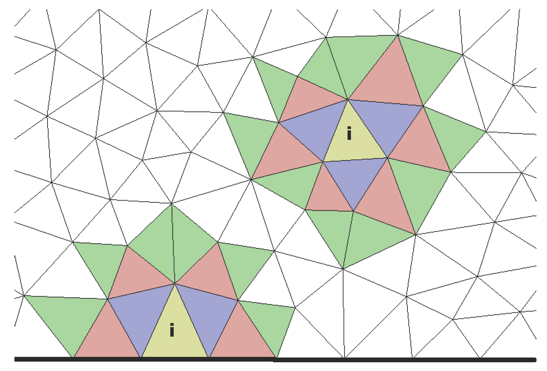
As the starting point of the collection algorithm, one big, central stencil is gathered. On arbitrary mapped meshes, the most compact stencil could be collected by using point-neighbour information. On the contrary, the use of face-neighbours extends the dependent data further into the mesh which reduces the redundancy of data on anisotropic, structured meshes [3]. The affine transformation preserves the principal connections between the cells for which reason the gathering can be performed using existing owner-neighbour lists. The most efficient way of collecting cells on unstructured meshes is based on adding the neighbours of the target cell iteratively until each stencil has the sought size. By collecting a surplus of possible stencil cells, the algorithm is independent of the starting point of an iteration and provides complete layers of new neighbours at a time as it is shown in Figure 1. The necessary size of the list $N_U$ relates to the number of internal faces of the target cell $L_i$ according to

$$\begin{array}{cc}\hfill N_U& =(L_i+1)·J_{max},\hfill \end{array}$$

(26)

which offers a small surplus due to the described collection of layers and in case of convoluted boundaries. After the selection of sectoral stencils, the central stencil is simply obtained by cutting it to the necessary size $J_{max}$. In general, the number of sectors equals the number of internal faces of $V_i^{\prime }$. However, if some sector does not provide enough cells it is not taken into account for the runtime operations. It may happen that more layers have to be considered until the necessary size is reached near boundaries. At this point, the iterative implementation is straightforward and advantageous. Once the lists are completed, all candidates are sorted by the centre to centre distances to the target cell in $\overrightarrow{\xi }$ and the nearest $N_U$ cells are stored.

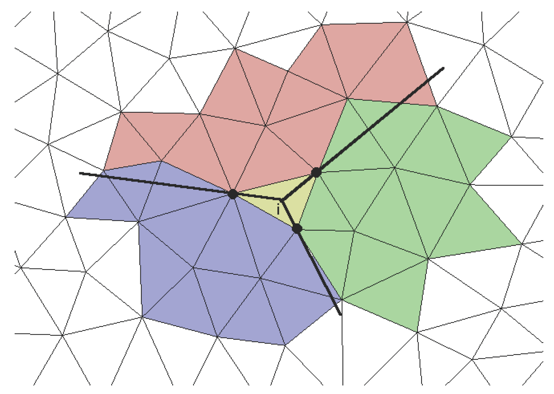
As the next step, sectoral stencils are constructed under consideration of the on condition that they are not allowed to share another cell than the target cell [3]. For this purpose, each sector is spanned as a cone with the cell centre of the target cell $P_0=(x_0,y_0,z_0)$ as the apex and the contour of the related face as the base. The $N_U$ cells are assigned to the sectors according to the position of their cell centres which results in a distribution as can be seen in Figure 2. In order to check the assignment of the cells, each sector is mapped to the first octant of another transformation space $\overrightarrow{X}=(X,Y,Z)$ where the relevant cell centres have positive coordinates (see [3] for details). The cell centre of each of the $N_U$ cells is transformed to $\overrightarrow{X}$ of every sectoral stencil and added to its list if

• All coordinates in the reference space are positive.
• The cell is not already a member of another stencil which may happen on Cartesian grids where the centre lies on the boundary of two adjunct sectors.
• The target stencil list contains no more than $J_{max}$ cells.

The first and last condition are simple requests while the second condition is prevented by using a dynamic list from which cells are removed after being assigned to a sector. The obtained stencils are compact by itself since the central lists are presorted and scanned from the nearest to the farthest cells.

2.2. Parallelisation

In this section, details of the parallelisation of the code are given. It is a crucial step due to the time-consuming reconstruction process at runtime. By default, OpenFOAM^® is based on a 0-halo approach which divides the domain into several non-overlapping regions and Message Passing Interface (MPI) to transmit the information between the inter-processor boundaries. This leads to at best second-order accurate solutions at such boundaries. In contrast, the stencils of a high-order (W)ENO scheme near processor patches need the geometrical and physical data from several layers of the neighbouring domain. Consequently, a n-halo approach with several overlapping sub-domains would be the proper choice. The implicit handling of the Navier-Stokes equations leads to algebraic systems of equations which are solved by linear, iterative solvers in OpenFOAM^®. Since these solvers only work for 0-halo approaches, a n-halo approach is discarded. Instead, the solution is the virtual extension of the sub-domains by collecting halo cells from neighbouring processors in additional lists. Then, the field values of the halo cells are updated at the beginning of each runtime step which is computed on non-overlapping domains.

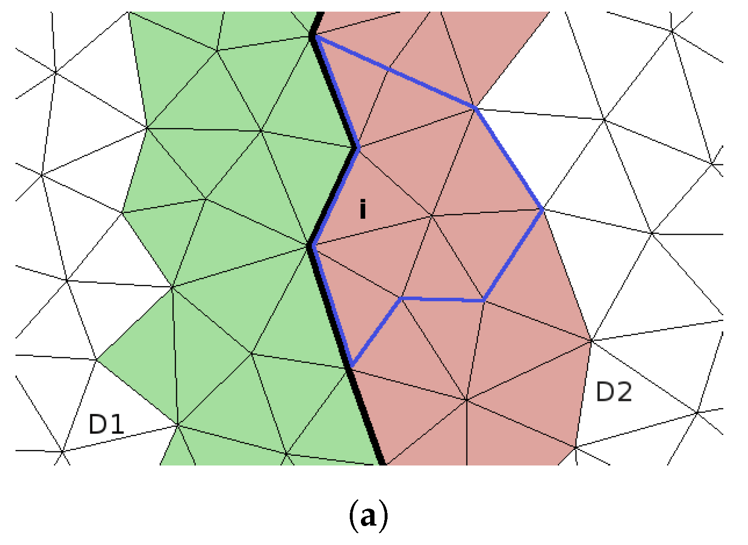
The initialization of parallelisation starts in the preprocessing step after the local stencils are collected. At this point, several stencils with a deformed shape exist near processor boundaries such as the blue framed stencil in Figure 3a. Appropriate halo cells from other processors provide the necessary correction of the stencils. It is noticeable that all possible stencils with a deformed shape and therefore, acceptors for halo cells, are included in the stencils of target cells next to processor boundaries. It implies that these acceptor cells are vice versa the only possible halo cells for stencils of other processors. Hence, the halo cells do not have to be collected separately but can just be taken from the prepared local stencil lists. This leads to the following modification of the central stencil collection algorithm (Section 2.1) in the case of using several processors:

• For each sub-domain $D_i$, all cells from the stencils of target cells next to a processor boundary are gathered in a list of halo cells together with the information of the target processor. Beyond, the stencils of these cells are marked as possible acceptors for halo cells from other sub-domains. In Figure 3a, acceptor cells of the sub-domain $D_1$ are coloured green while its halo cells from sub-domain $D_2$ are coloured red and vice versa the green cells are the halo cells from sub-domain $D_1$ for the red acceptor cells of $D_2$.
• The lists of halo cells are further prepared by assigning them a new ID and additionally, storing their cell centre coordinates and the coordinates of the triangles from the triangulation of the cell’s boundaries. Afterwards, the lists are transmitted to the appropriate target processor using MPI.
• The required halo cells for each marked central stencil $S_{c,i}$ are determined by a geometrical selection due to missing face neighbour information beyond processor boundaries. For this purpose, a sphere is spanned around the target cell $V_i^{\prime }$ of $S_{c,i}$ with the distance from the centre of $V_i^{\prime }$ to the outermost cell centre in the local stencil as the radius. All halo cells whose cell centres are located within this sphere are added to a new global stencil. In Figure 3b, this geometrical selection results in the yellow coloured global stencil for the blue framed stencil in Figure 3a.
• The final stencils are attained from sorting the global stencils by distance and pick the nearest $J_{max}$ cells. In Figure 3b, the new stencil is framed in blue.

Additional lists with the information of the origin processor of each cell in a stencil are generated in order to transmit the field data between processors before the local reconstruction starts in each runtime step. It might be noticed that the results of a reconstruction on multiple processors are minimally different to results of serial calculations due to the slightly different stencils [13]. The stencil collecting algorithm through processor boundaries uses geometrical searching while on a single processor just the face neighbours are gathered.

3. Derivation of Semi-Implicit WENO-based Convection Schemes

The reconstruction of any function in multiple dimensions and on unstructured meshes can be computed using the above presented WENO reconstruction method. In the following sections, possible discretisation schemes are derived which are all generally applicable in the high-level use of OpenFOAM^® (The presented interpolations are, however, limited to the surface interpolation class of OpenFOAM^® which stands in contrast to the point interpolation class).

In FVM, any convective term is discretised applying volume integration over each cell and Gauss’s theorem for transforming the arising volume integrals in a sum of surface integrals over all faces $L_i$ of cell $V_i$,

$$\begin{array}{cc}\hfill {\int }_{V_i}\nabla \left(\overrightarrow{u}\Phi \right)\mathrm{d}V& =\sum _l^{L_i}{\int }_{F_l}{\overrightarrow{n}}_l\overrightarrow{u}\Phi \mathrm{d}{F}_l.\hfill \end{array}$$

(27)

In case of a high-order scheme, the integrals in (27) have to be evaluated with a Gaussian integration of higher order, too. The velocity at the face are taken out of the integration since (27) is always treated in a linearised form here. Inserting the polynomial expressions of $\Phi$ (16) in (27) yields at any face $F_l$ of $V_i$

$$\begin{array}{cc}\hfill {\int }_{F_l}{\overrightarrow{n}}_l\overrightarrow{u}\Phi \mathrm{d}{F}_l& ={\overrightarrow{u}}_l·\frac{{\overrightarrow{n}}_l\left|F_l\right|}{\left|F_l^{\prime }\right|}{\int }_{F_l^{\prime }}\Phi \mathrm{d}{F}_l^{\prime }=\frac{Q_l}{\left|F_l^{\prime }\right|}{\int }_{F_l^{\prime }}{p}_i\mathrm{d}{F}_l^{\prime }\hfill \\ & =Q_l·\left[{\overline{\Phi }}_i+\frac{1}{\left|F_l^{\prime }\right|}·\left(\sum _{k=1}^K{\tilde{a}}_{k,i}·{\int }_{F_l^{\prime }}{\Omega }_{k,i}\left(\overrightarrow{\xi }\right)\mathrm{d}{F}_l^{\prime }\right)\right],\hfill \end{array}$$

(28)

with $Q_l$ the volumetric flow rate (Since the common gaussian integration of OpenFOAM^® is limited to second order of accuracy, the basis classes multiply the results of the interpolation by the face areas. Therefore, we neglect the surface area in (28) in the implementation in order stay consistent). The remaining surface integrals in (28) are solution independent and can be precomputed. Under consideration of (5), they are expressed as

$$\begin{array}{cc}\hfill {\int }_{F_l^{\prime }}{\Omega }_{k,i}\mathrm{d}{F}_l^{\prime }& ={\int }_{F_l^{\prime }}{\Psi }_k\mathrm{d}{F}_l^{\prime }-{\displaystyle \frac{\left|F_l^{\prime }\right|}{\left|V_i^{\prime }\right|}}{\int }_{V_i^{\prime }}{\Psi }_k\mathrm{d}{V}_i^{\prime }.\hfill \end{array}$$

(29)

The volume integrals in (29) are already computed during the reconstruction procedure. The surface integrals over the basis functions are evaluated in a similar way by decomposing the faces into triangles and using Gaussian quadrature rules of appropriate order. Hence, the evaluation of linearised convective terms reduces to a sum of scalar products at runtime, at which the considered polynomials depend on the chosen flux evaluation procedure.

The flux evaluation of linearised convective terms can be interpreted as the flux solution of the Riemann problem for the linear advection equation which is defined as [28]

$$\begin{array}{cc}\hfill {\displaystyle \frac{\partial \Phi }{\partial t}}+\nabla ·\left(\Phi \overrightarrow{u}\right)& =0,\hfill \end{array}$$

(30)

under consideration of an incompressible fluid. Its finite volume formulation arises similar to (27) as

$$\begin{array}{cc}\hfill {\displaystyle \frac{d}{dt}}{\overline{\Phi }}_i+{\displaystyle \frac{1}{\left|V_i\right|}}\sum _l^{L_i}{\int }_{F_l}\widehat{F}\mathrm{d}{F}_l& =0,\hfill \end{array}$$

(31)

with the numerical flux $\widehat{F}$

$$\begin{array}{cc}\hfill \widehat{F}& =\left(\overrightarrow{u}·{\overrightarrow{n}}_l\right)\Phi =u_{n_l}\Phi .\hfill \end{array}$$

(32)

Toro [28] showed that the flux evaluation in (31) can be executed in the normal direction of each face $n_l$ due to its rotational invariance. Thereby, it is represented at each face by the one-dimensional equation

$$\begin{array}{cc}\hfill {\displaystyle \frac{\partial \Phi }{\partial t}}+{\displaystyle \frac{\partial \widehat{F}}{\partial n_l}}& =0,\hfill \end{array}$$

(33)

resulting in the Riemann problem [28]

$$\begin{array}{c}\hfill \left.\begin{array}{cc}\mathrm{PDE}:\hfill & {\displaystyle \frac{\partial \Phi }{\partial t}}+u_{n_l}{\displaystyle \frac{\partial \Phi }{\partial n_l}}=0,\hfill \\ \mathrm{IC}:\hfill & \Phi (n_l,0)={\Phi }_0\left(n_l\right)=\left\{\begin{array}{ccc}{\Phi }^{-}\hfill & \mathrm{if}\hfill & n_l<0\hfill \\ {\Phi }^{+}\hfill & \mathrm{if}\hfill & n_l>0\hfill \end{array}\right.\hfill \end{array}\right\},\end{array}$$

(34)

with the initial data ${\Phi }^{\pm }$ representing the values of $\Phi$ from the adjacent cells at one point of the considered face. Taking the exact solution of (34) [28] into account, the flux yields at the face ($n_l=0$) at any time $t>0$

$$\widehat{F}=\left\{\begin{array}{ccc}{u}_{n_l}{\Phi }^{-}\hfill & \mathrm{if}\hfill & u_{n_l}>0\hfill \\ u_{n_l}{\Phi }^{+}\hfill & \mathrm{if}\hfill & u_{n_l}<0\hfill \end{array}\right..$$

(35)

These fluxes result in an unconditional stable solution for which reason the Riemann solver (35) is appropriate for creating high-order interpolation methods based on WENO reconstructions. As proposed by Toro [29], we extend Godunov’s first-order version, which is based on cell centre values of ${\Phi }^{\pm }$, by higher-order terms of the reconstruction; the so-called WENOUpwindFit arises as a high-order non-oscillatory upwind scheme. For this purpose, the two reconstructed face values ${\Phi }^{-}$ and ${\Phi }^{+}$ are recalled from above (compare (16))

$$\begin{array}{cc}\hfill {\Phi }^{-}({\overrightarrow{\xi }}^{-})& ={\overline{\Phi }}_i+\sum _{k=1}^K{\tilde{a}}_{k,i}·{\Omega }_{k,i}({\overrightarrow{\xi }}^{-}),\hfill \\ \hfill {\Phi }^{+}({\overrightarrow{\xi }}^{+})& ={\overline{\Phi }}_{jl}+\sum _{k=1}^K{\tilde{a}}_{k,jl}·{\Omega }_{k,jl}({\overrightarrow{\xi }}^{+}).\hfill \end{array}$$

(36)

Here, the index i represents the owner and $jl$ represents the neighbour cell of the face. The correlating reference spaces are denoted by ${\overrightarrow{\xi }}^{\pm }$. The sought fluxes can be evaluated from (27) and (35) as

$$\begin{array}{cc}\hfill {\int }_{F_l}{\overrightarrow{n}}_l\overrightarrow{u}\Phi \mathrm{d}{F}_l& =\left\{\begin{array}{ccc}{\int }_{F_l}{\overrightarrow{n}}_l\overrightarrow{u}{\Phi }^{-}\mathrm{d}{F}_l\hfill & \mathrm{if}\hfill & u_{n_l}>0\hfill \\ {\int }_{F_l}{\overrightarrow{n}}_l\overrightarrow{u}{\Phi }^{+}\mathrm{d}{F}_l\hfill & \mathrm{if}\hfill & u_{n_l}<0\hfill \end{array}\right.,\hfill \end{array}$$

(37)

with the polynomials (36) instead of ${\Phi }^{\pm }$. The surface integrals are evaluated using (28) in the proper reference space.

So far, most WENO schemes were used explicitly. However, the presented method can also be applied as a deferred correction method [30] which combines an implicit first-order upwind scheme with an explicit high-order correction term. The first-order part ensures convergence due to its monotonicity and diagonal dominance. The required subdivision is already available as can be seen in (36). This semi-implicit WENO scheme fits in the most solution algorithms of OpenFOAM^® such as SIMPLE or PISO. Unfortunately, as it is shown in [31], WENO schemes are not strictly bounded. The explicit correction term can, therefore, be unbounded and still influence the solution’s physical reliability.

In order to overcome possible issues with unbounded solutions, the limiting strategy of Zhang and Shu [7], which can be applied to any high-order finite volume scheme in order to satisfy the maximum-principle for scalar conservation laws, is adapted to the presented scheme . The property implies that a time step’s solution is bounded by the cell centred values of the previous step. Hence, it is important for the convergence to the entropy solution. It might be noticed, that all monotone and TVD schemes fulfil the maximum-principle but lose accuracy at smooth extrema due to the measuring of the total variation using the cell centred values. In contrast, the new limiter is evaluated from the maximum and minimum of the reconstruction polynomials in each cell which preserves the accuracy. I was shown [7] that the limited WENO polynomial ${\tilde{p}}_i(\overrightarrow{\xi })$ fulfils the maximum-principle by applying a linear scaling limiter ${\theta }_i\in [0,1]$ to the polynomial $p_i(\overrightarrow{\xi })$ of cell $V_i^{\prime }$ in accordance to

$$\begin{array}{cc}\hfill {\tilde{p}}_i& ={\theta }_i·p_i+\left(1-{\theta }_i\right)·{\overline{\Phi }}_i,\hfill \\ \hfill {\theta }_i& =\min \left(\left|{\displaystyle \frac{M-{\overline{\Phi }}_i}{M_i-{\overline{\Phi }}_i}}\right|,\left|{\displaystyle \frac{m-{\overline{\Phi }}_i}{m_i-{\overline{\Phi }}_i}}\right|,1\right).\hfill \end{array}$$

(38)

Here, M and m are defined as the upper and lower global bounds of $\overline{\Phi }$. The local minimum and maximum is calculated as [7]

$$\begin{array}{cc}\hfill M_i(\overrightarrow{\xi })& =\underset{\overrightarrow{\xi }\in V_i^{\prime }}{\max }{p}_i(\overrightarrow{\xi }),\hfill \\ \hfill m_i(\overrightarrow{\xi })& =\underset{\overrightarrow{\xi }\in V_i^{\prime }}{\min }{p}_i(\overrightarrow{\xi }).\hfill \end{array}$$

(39)

The values in (39) should be evaluated from the polynomials at all Gaussian points at runtime. In the presented interpolation scheme, the surface integration is precomputed for which reason this handling would be inefficient. It is, therefore, decided to take the surface integrated values of $p_i$ into account instead. This decision is towards the underlying mathematics, but on the other hand, the values of M and m are also just available at the cell centres in OpenFOAM^®. Hence, Equation (39) is evaluated as

$$\begin{array}{cc}\hfill M_i(\overrightarrow{\xi })& =\underset{l}{\max }\left(\frac{1}{\left|F_l^{\prime }\right|}{\int }_{F_l^{\prime }}{p}_i(\overrightarrow{\xi })\mathrm{d}{F}_l^{\prime }\right),\hfill \\ \hfill m_i(\overrightarrow{\xi })& =\underset{l}{\min }\left(\frac{1}{\left|F_l^{\prime }\right|}{\int }_{F_l^{\prime }}{p}_i(\overrightarrow{\xi })\mathrm{d}{F}_l^{\prime }\right),l=1,\dots ,L_i.\hfill \end{array}$$

(40)

By limiting the integrated polynomials, the interpolation scheme can be rewritten as a sum of a first-order upwind scheme and a limited high-order correction. For the sake of practicability, another user specified parameter ${\theta }_2\in [0,1]$ is introduced which provides the switch between a limited (${\theta }_2=1$) and unlimited (${\theta }_2=0$) computation. Hence, the final fluxes of the WENOUpwindFit scheme become (compare (28))

$$\begin{array}{cc}\hfill {\int }_{F_l}{\overrightarrow{n}}_l& \overrightarrow{u}\Phi \mathrm{d}{F}_l=Q_l·\left[{\theta }_2·\left\{{\overline{\Phi }}_i+\frac{{\theta }_i}{\left|F_l^{\prime }\right|}·\left(\sum _{k=1}^K{\tilde{a}}_{k,i}·{\int }_{F_l^{\prime }}{\Omega }_{k,i}(\overrightarrow{\xi })\mathrm{d}{F}_l^{\prime }\right)\right\}+\right.\hfill \\ & \left.(1-{\theta }_2)·\left\{{\overline{\Phi }}_i+\frac{1}{\left|F_l^{\prime }\right|}·\left(\sum _{k=1}^K{\tilde{a}}_{k,i}·{\int }_{F_l^{\prime }}{\Omega }_{k,i}(\overrightarrow{\xi })\mathrm{d}{F}_l^{\prime }\right)\right\}\right].\hfill \end{array}$$

(41)

As an alternative, WENO reconstructions can also be used for the implementation of central schemes which evaluate the fluxes as follows

$$\begin{array}{cc}\hfill {\int }_{F_l}{\overrightarrow{n}}_l\overrightarrow{u}\Phi \mathrm{d}{F}_l& ={\int }_{F_l}{\overrightarrow{n}}_l\overrightarrow{u}·\left(w_{CD,l}{\Phi }^{-}+(1-w_{CD,l})·{\Phi }^{+}\right)\mathrm{d}{F}_l,\hfill \end{array}$$

(42)

with ${\Phi }^{\pm }$ from (36) and $w_{CD,l}$ the central differencing weights. Analogue to the upwind scheme, this scheme is the combination of an implicit central-differencing discretisation and a central high-order correction term. The scheme is not monotone and may lead to divergence of the solution in case of convection dominant flows [32] and hyperbolic equations, respectively, due to the negligence of characteristic curves. More stable centred schemes can generally be build from WENO reconstructions but are not in the scope of this research (see e.g., in [33,34,35]).

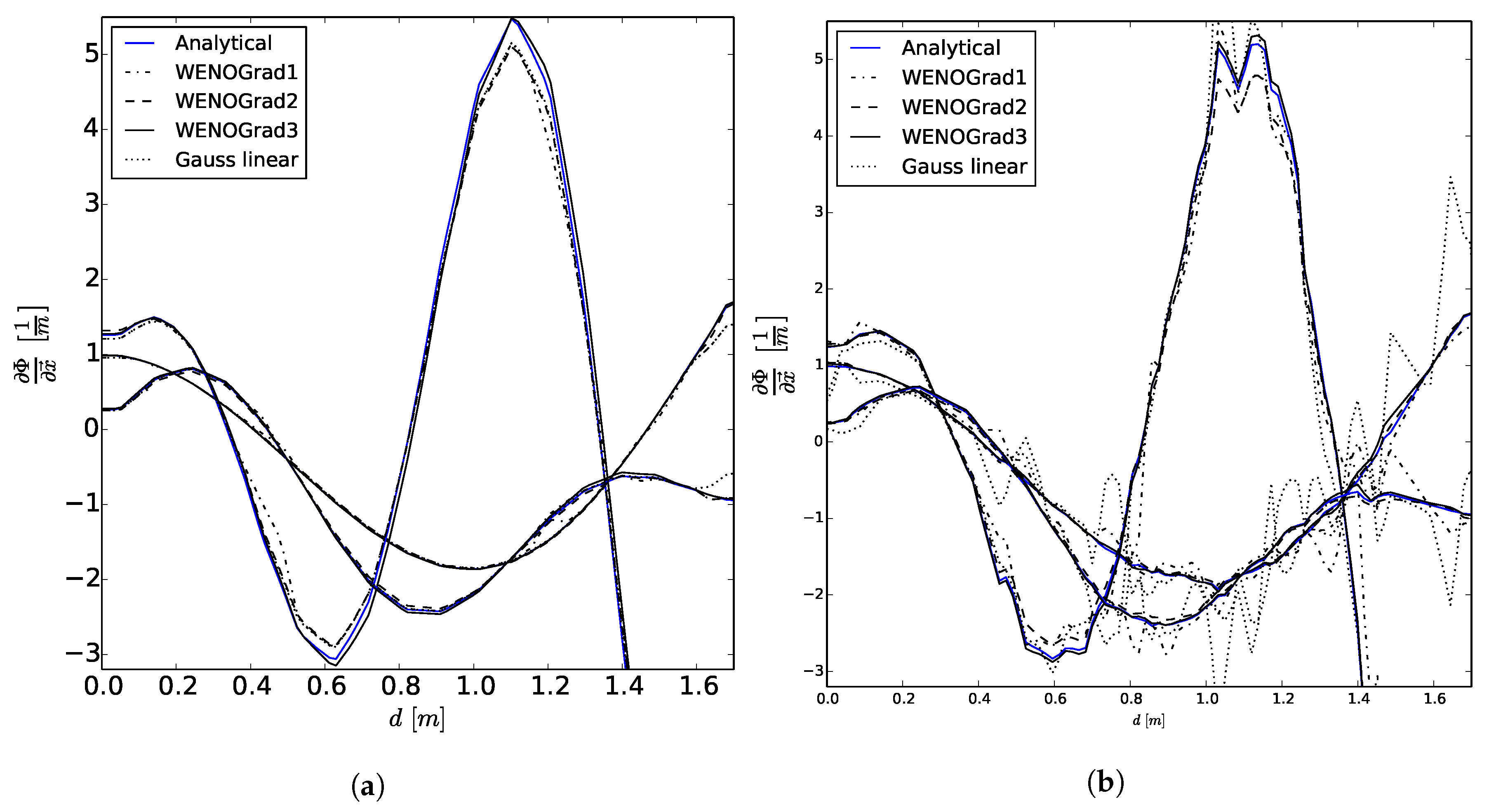
4. Derivation of a WENO Gradient Scheme

The calculation of gradients in the cell centres is a frequent operation in FVM. Besides the standard discretisation using Gauss’s theorem and linear interpolation, OpenFOAM^® offers a least-squares-based gradient scheme whose stencils are however limited to the first neighbours. On the contrary, the presented scheme takes a larger stencil into account and avoids spurious oscillations at the same time. Alternatively, the WENO weighting could also be skipped in order to get a high-order version of the existing least-squares method.

The starting point of the gradient calculation in the cell centre of $V_i$ is its finite volume formulation

$$\begin{array}{cc}\hfill {\left(\nabla \Phi \right)}_i& ={\displaystyle \frac{1}{\left|V_i\right|}}{\int }_{V_i}\nabla \Phi \mathrm{d}V.\hfill \end{array}$$

(43)

The volume integral in (43) can be evaluated with a high-order accuracy in two ways. One opportunity is the transformation into surface integrals and a high-order interpolation of $\overline{\Phi }$ to the boundaries using e.g., the central WENO scheme. This method is applicable without any further derivations and superior to linear interpolation due to the mesh independence. A more efficient computation is the direct evaluation of the volume integral by replacing the gradient of $\Phi$ by its polynomial representation using WENO reconstructions. Here, the difficulty is the correct definition of the Gaussian points in arbitrary shaped volumes which could be obtained by decomposing each cell in tetrahedra where the Gaussian points are known. The coordinates and weights could be stored in the preprocessing resulting in higher efficiency in runtime. However, the additional tetrahedralization is a time-consuming computation and should be avoided. If the non-oscillatory behaviour of the scheme is in the first place and the theoretical order of accuracy is less important, a more efficient gradient scheme can be derived by replacing the gradient of $\Phi$ by its polynomial representation and evaluating the volume integral with second order of accuracy. It corresponds to the evaluation of the gradient at the centre ${\overrightarrow{x}}_i$ of $V_i$ according to

$$\begin{array}{cc}\hfill {\displaystyle \frac{1}{\left|V_i\right|}}{\int }_{V_i}\nabla \Phi \left(\overrightarrow{x}\right)\mathrm{d}V& \approx \nabla \Phi {|}_{\overrightarrow{x}={\overrightarrow{x}}_i}.\hfill \end{array}$$

(44)

The resulting gradients are a compromise between accuracy, stability and efficiency due to its simple evaluation without any integrations. They have to be further transformed into the reference space in accordance with the polynomials of the WENO reconstruction. As given in [3], the gradient at ${\overrightarrow{x}}_i$ yields then

$$\begin{array}{cc}\hfill {\nabla }_{\overrightarrow{x}}\Phi {|}_{\overrightarrow{x}={\overrightarrow{x}}_i}& ={\left({\mathcal{J}}^{-1}\right)}_i^T·{\nabla }_{\overrightarrow{\xi }}\Phi {|}_{\overrightarrow{\xi }={\overrightarrow{\xi }}_i},\hfill \end{array}$$

(45)

due to the affine transformation. ${\nabla }_{\overrightarrow{\xi }}$ represents the gradients in the principal directions of the reference space. Next, $\Phi$ is replaced by its polynomial Formulation (16), derivatives are taken and $\overrightarrow{\xi }={\overrightarrow{\xi }}_i$ is inserted. The formula can then be simplified due to the cell centred orthogonal basis functions (see [27] for details). The remaining non-zero terms are related to the coefficients of the first-order terms of the polynomial, so that the final expression reads as follows

$$\begin{array}{cc}\hfill {\nabla }_{\overrightarrow{x}}\Phi {|}_{\overrightarrow{x}={\overrightarrow{x}}_i}& ={\left({\mathcal{J}}^{-1}\right)}_i^T·{\left(\begin{array}{c}{\tilde{a}}_3\\ {\tilde{a}}_2\\ {\tilde{a}}_1\end{array}\right)}_i.\hfill \end{array}$$

(46)

The inverse Jacobian matrices are already calculated in the mapping process during the preprocessing. The resulting gradient scheme, called WENOGrad, can be applied to any gradient computation in OpenFOAM^® due to its explicit treatment in any case.

5. Implementation of the WENO Schemes in OpenFOAM^®

In the following, several details of the implementation in the framework of OpenFOAM^® are provided. The main accomplishment of this step is embedding the new methodology in the existing code structure such that all schemes are applicable in the same way as the existing low-order methods.

5.1. Preprocessing

The preprocessing of high-order WENO schemes is a time-consuming procedure including the extended stencil collection, calculation of multiple smoothness and reconstruction matrices, and several SVD computations for each cell. Assuming a time-invariant mesh, all steps just have to be computed once before the first runtime reconstruction is performed. Therefore, a singleton pattern is implemented which restricts the instantiation of the preprocessing class, called WENOBase, to a single object [36]. To that effect, the preprocessing functions can just be called once at runtime. Here, one object is created which holds all necessary lists. In all following time steps, the singleton pattern not only prevents the creation of further instances but also provides global access to the held lists of the unique instance. The executed preprocessing steps are under consideration of Section 2:

• Generation of one large central stencil list for each control volume $V_i^{\prime }$ in the transformed space and sorting it by distance as described in Section 2.1.
• Calculation and storing of all volume integrals of the basis functions of $V_i^{\prime }$ using triangularization of the faces and a Gaussian quadrature rule of appropriate order.
• If several processors are involved, halo cells are collected. Afterwards, appropriate cell coordinates and triangulated face coordinates are transmitted and the global stencils are gathered using the procedure of Section 2.2.
• Generation of the sectoral stencils and the final central stencil in accordance with the algorithm described in Section 2.1.
• Determination of the reconstruction matrix for each sectoral stencil of $V_i^{\prime }$ (see (21)). For this purpose, volume integrals of the basis functions for the cells in the stencil are calculated in the space of $V_i^{\prime }$. Finally, the pseudoinverse ${\mathcal{A}}^{+}$ is computed using SVD.
• Calculation of the oscillation indicator matrix $\mathcal{B}$ for each $V_i^{\prime }$ using (14).

The efficiency of the preprocessing is further improved by storing the lists of the most time-consuming processes as files in the constant folder of the considered case. During a restart of the simulation, the WENOBase class searches for these lists and read them if available.

5.2. Runtime

The runtime operations of the reconstruction are performed in the WENOCoeff class (see Figure 4). The input data is any variable $\Phi$ represented by the averaged values of each cell ${\overline{\Phi }}_i$. The first step consists of calling the WENOBase class in order to check whether an object already exists. The constructor of the preprocessing class returns the object directly or after the preprocessed lists are newly created and read from written files, respectively. The necessary lists are then obtained in each time step by calling a designated function. Afterwards, the following runtime steps are executed:

• Collection and transmission of the field values of the halo cells in case of parallel computing.
• For each stencil of $V_i^{\prime }$, generation of the vector b as the right hand side of (19) using $\overline{\Phi }$. The degrees of freedom $a_k^{\left(m\right)}$ are then computed directly from a matrix vector product using ${\mathcal{A}}^{+}$.
• Insertion of the coefficients in (10) and evaluation of the smoothness indicator afterwards.
• Calculation of the WENO weights using (8) and computation of the modified degrees of freedom. Under consideration of (16), this evaluation can be written as

  $$\begin{array}{cc}\hfill {\tilde{a}}_k& =\sum _{m=0}^{N_{Si}}{\omega }_m{a}_k^{\left(m\right)}.\hfill \end{array}$$

  (47)

All derived schemes obtain the necessary information for building the polynomials by this procedure which facilitates the addition of new schemes by users easily. The order of accuracy of the schemes are not restricted by the presented algorithm for which reason the polynomial order r is an user defined parameter. For the sake of convenience, r is defined in the default file for the selection of all schemes (fvSchemes). Exemplary entries look as follows

$$\begin{array}{c}\mathrm{grad}\left(\mathrm{alpha}\right)\mathrm{WENOGrad} 2;\hfill \\ \mathrm{div}(\mathrm{phi},\mathrm{alpha})\mathrm{Gauss} \mathrm{WENOUpwindFit}2 0;\hfill \end{array}$$

The first entry corresponds to a gradient discretisation based on a second-order polynomial and the second entry to the discretisation of a convection term using Gauss’s theorem and the third-order accurate WENOUpwindFit interpolation scheme. The last entry is related to the limiting strategy in (41).

6. Verification

In the following, the presented implementation is verified by evaluating the accuracy of the WENO reconstruction and the WENO convection scheme applied to the advection equation.

6.1. Accuracy of Reconstruction for Smooth Functions

The order of accuracy $\alpha$ corresponds to the relation between the ${\mathcal{L}}_p$-norm of the error and different grid resolutions. It is represented as the slope of the line through the corresponding points of error and mesh size in a log-log plot. Knowing the error norm for two grids ${\mathcal{L}}_{p1}$ and ${\mathcal{L}}_{p2}$ with the characteristic sizes ${\Delta }_1$ and ${\Delta }_2$, the order of accuracy $\alpha$ is obtained as

$$\alpha ={\displaystyle \frac{log\left(\frac{{\mathcal{L}}_{p2}}{{\mathcal{L}}_{p1}}\right)}{log\left(\frac{{\Delta }_2}{{\Delta }_1}\right)}}.$$

(48)

The characteristic size is taken as $\sqrt[3]{N}$ in 3D and $\sqrt{N}$ in 2D with N the total number of cells in the domain. The ${\mathcal{L}}_2$-norm of error is considered which is calculated as

$$\begin{array}{cc}\hfill {\mathcal{L}}_2=& \sqrt{{\displaystyle \frac{1}{\left|V_T\right|}}\sum _{i=1}^N\underset{V_i}{\int \int \int }{\left(p_i\left(\overrightarrow{x}\right)-{\Phi }_{exact}\left(\overrightarrow{x}\right)\right)}^2\mathrm{d}x\mathrm{d}y\mathrm{d}z},\hfill \\ & i=1,\dots N,\hfill \end{array}$$

(49)

with $\left|V_T\right|$ the total volume of the domain and ${\Phi }_{exact}\left(\overrightarrow{x}\right)$ the known exact solution in $\left|V_T\right|$. The polynomials $p_i\left(\overrightarrow{x}\right)$ are computed from (16) with appropriate space transformations. The volume integrals in (49) are evaluated by a transformation into surface integrals and the use of Gaussian quadrature rules from above with a higher order than in the reconstruction. For this purpose, an integration of the differences over one of the coordinates has to be executed analytically. This can be computed by any mathematical software package for sufficient simple functions. The grids are generated without changing the topology during the refinement steps to prevent the results from additional scaling effects. For the two-dimensional calculations, hexahedral and triangular meshes are considered. In 3D, hexahedral and non-regular tetrahedral grids are taken into account. All meshes are presented in form of their coarsest grid resolution in Figure 5 and Figure 6, respectively.

First, a smooth two-dimensional function is reconstructed using WENO reconstructions with polynomials of first- to fourth-order. No analytical integration has to be executed since the integrals in (48) simplify to surface integrals for two-dimensional cases. The considered function is taken from McDonald [12] which offers the possibility of comparing the results to another high-order approach. The central essential non-oscillatory (CENO) scheme is based on a least squares reconstruction and an additional limiter in order to prevent oscillations. The function is given as

$${\Phi }_{exact}(x,y)=1+{\displaystyle \frac{1}{3}}·\cos \left(\sqrt{x^2+y^2}\right).$$

(50)

The solution is computed on a quadratic domain with an edge length of 20 and centred on $x=y=0$. In Figure 7a, the initial data is shown on a structured grid with 2500 hexahedra.

The results of the reconstructions are shown in Figure 8 where the ${\mathcal{L}}_2$-norm of the error is plotted over the characteristic size. As expected, the accuracy of the scheme increases with raising polynomial order and grid resolution. Further, the results are almost the same for both cell shapes except for first-order. The fourth-order accurate CENO scheme from calculations on unstructured grids is outperformed by the corresponding WENO scheme which indicates the conservation of an accurate smooth solution by the WENO weighting in comparison to limiting strategies. The order of accuracy is evaluated for the ${\mathcal{L}}_2$-norm of the error under consideration of (48) and presented in

Table 1. Order of accuracy from the numerical convergence study for the smooth, two-dimensional function on hexahedral ${\alpha }_{hex}$ and triangular ${\alpha }_t$ grids using ${\mathcal{L}}_2$.

Polynomial Order r	${\mathit{\alpha }}_{\mathit{hex}}$	${\mathit{\alpha }}_{\mathit{t}}$
1	$2.1$	$1.7$
2	$3.1$	$3.2$
3	$4.7$	$4.7$
4	$6.2$	$5.1$

. Obviously, the scheme reaches the nominal convergence rate of common numerical methods and even exceeds it for higher-order polynomials which is consistent with the theoretically possible order of WENO reconstructions.

Next, a smooth, three-dimensional function is reconstructed using polynomials of first- to third-order. The function is harmonically with changes in all three coordinate directions

$${\Phi }_{exact}(x,y,z)=y·\cos \left(4x\right)+z·\sin \left(10y\right)+x·\cos \left(3z\right).$$

(51)

The solution is computed on a cubic domain with an edge length of 1 m and centred on $x=y=z=0.5$ m. The initial data on a hexahedral grid with 8000 hexahedra is shown in Figure 7. In Figure 9, the resulting ${\mathcal{L}}_2$-norm of the error is shown for increasing grid resolutions. Generally, the scheme provides the expected distribution of the norm for increasing order and resolution. The evaluation of the order of accuracy from the convergence study of the ${\mathcal{L}}_2$-norm of the error is shown in

Table 2. Order of accuracy from the numerical convergence study for the smooth, three-dimensional function on hexahedral ${\alpha }_{hex}$ and tetrahedral ${\alpha }_{tet}$ grids using ${\mathcal{L}}_2$.

Polynomial Order r	${\mathit{\alpha }}_{\mathit{hex}}$	${\mathit{\alpha }}_{\mathit{tet}}$
1	$2.0$	$1.9$
2	$3.1$	$3.3$
3	$4.1$	$4.2$

. The nominal order can be reached for both meshes and all polynomial orders. However, the convergence of the scheme is slightly better on unstructured grids as well.

6.2. Numerical Convergence Study of the Advection Equation

A verification of the WENO upwind-biased convection scheme WENOUpwindFit is presented for the advection equation. This Equation (30) is introduced in Section 3 for deriving the exact Riemann solver for the WENO scheme. The spatial discretisation of the equation’s finite volume Formulation (31) is handled by the first- to third-order unlimited WENOUpwindFit scheme as well as the TVD scheme with van Leer’s limiter (TVD-vanLeer) as a reference. The temporal discretisation is performed explicitly using the TVD third-order accurate Runge-Kutta method [37]. The time step has to be chosen without violating the stability of WENO which is a restriction on the CFL-condition to $CFL\le \frac{1}{3}$ in three dimensions [34]. The initial field is calculated from sine functions as [38]

$$\Phi (x,y,z)=\sin (\pi ·(x+y+z\left)\right)+\sin (2\pi ·(x+y+z\left)\right).$$

(52)

It is transported with the velocity field $\overrightarrow{u}=(2\frac{m}{s},2\frac{m}{s},2\frac{m}{s})$ in a cubic domain of 2 m × 2 m × 2 m with periodic boundary conditions. Hence, the field should match the initial distribution after t = 1 s. The considered meshes are hexahedral and tetrahedral containing between 4000 and 130,000 cells. As results, the ${\mathcal{L}}_2$-norm of error (49) is evaluated in a second-order accurate framework. This reduces the calculated convergence rate theoretically but provides the possibility to compare with the TVD method. Both, the norm of error and the convergence rate $\alpha$ are given in

Table 3. Error and convergence of WENO convection schemes for the advection equation on hexahedral meshes.

Convection Scheme	Number of Cells	${\mathcal{L}}_2$-Norm of Error	$\mathit{\alpha }$
TVD-vanLeer	4096	$0.75$	-
	27,000	$0.41$	$0.96$
	64,000	$0.25$	$1.62$
	125,000	$0.17$	$1.75$
WENO1	4096	$0.88$	-
	27,000	$0.62$	$0.57$
	64,000	$0.34$	$2.07$
	125,000	$0.21$	$1.98$
WENO2	4096	$0.7$	-
	27,000	$0.25$	$1.67$
	64,000	$0.10$	$3.13$
	125,000	$0.05$	$2.95$
WENO3	4096	$0.66$	-
	$\mathrm{27,000}$	$0.12$	$2.66$
	$\mathrm{64,000}$	$0.05$	$3.35$
	$\mathrm{125,000}$	$0.02$	$3.86$

and

Table 4. Error and convergence of WENO convection schemes for the advection equation on tetrahedral meshes.

Convection Scheme	Number of Cells	${\mathcal{L}}_2$-Norm of Error	$\mathit{\alpha }$
TVD-vanLeer	4188	$0.83$	-
	30,255	$0.64$	$0.39$
	58,456	$0.49$	$1.2$
	133,026	$0.31$	$1.75$
WENO1	4188	$0.87$	-
	30,255	$0.56$	$0.65$
	58,456	$0.29$	$2.94$
	133,026	$0.16$	$2.26$
WENO2	4188	$0.76$	-
	30,255	$0.35$	$1.17$
	58,456	$0.21$	$2.22$
	133,026	$0.09$	$3.1$
WENO3	4188	$0.53$	-
	30,255	$0.04$	$3.95$
	58,456	$0.02$	$4.38$
	133,026	$0.006$	$3.34$

for the hexahedral and tetrahedral meshes, respectively. On the structured grids, all WENO schemes can reach the nominal order if the resolution is not too coarse. This phenomenon for high order schemes has also been reported by other authors [3]. The TVD methods also shows an increasing convergence rate and similar error norms as the first-order WENO scheme, which confirms the expectation since both methods are second-order accurate. For all grids, the third-order WENO method has the smallest norm of error which demonstrates the convergence of the implementation as the polynomial order is increased. On the tetrahedral grids, the first- and third-order WENO schemes perform slightly better than on the hexahedral grids which might be caused by the better conditioned matrices on unstructured grids [14]. On regular hexahedral grids, almost linear dependent lines arise from the information of collinear cells. In comparison, the TVD method performs worse than before which presents evidence for the importance of the mapping. The first-order WENO scheme can, hence, outperform the standard method.

7. Applications

The previous verification procedure showed that the theoretical order of accuracy can be reached using the presented WENO method. In the following, the schemes are validated for different test cases to emphasise the principal working of the implementation. Special attention is paid to the advection equation and an application to two-phase flows. A performance comparison provides an additional tool for evaluating the overall performance of the schemes.

7.1. Application to the Gradient Calculation

The accuracy of the WENO gradient scheme (Section 4) shall be presented for a smooth, three-dimensional function with large gradients in all three coordinate directions. For this purpose, the first- to third-order WENOGrad scheme and OpenFOAM^®’s standard method, selectable as Gauss linear, are applied to the harmonic Function (51) of Section 6.1.

The solutions for the gradients of (51) are computed on a cubic domain with an edge length of 1 m and centred on (0.5 m, 0.5 m, 0.5 m). The considered meshes are a structured grid with 5800 cells and a tetrahedral grid with ≈6000 cells. The results are represented as a plot of the gradients of $\overline{\Phi }$ along the diagonal from (0 m, 0 m, 0 m) to (1 m, 1 m, 1 m) and can be seen in Figure 10. Here, all three gradients are pictured in a single figure for each mesh. The resulting curve of the third-order WENO gradient scheme coincides well with the analytical solution for this resolution regardless of the considered direction or mesh. The first- and second-order schemes as well as the reference method perform similar on the structured grid, which is slightly worse than WENOGrad3 if the gradients have a maximum or minimum. On the unstructured grid, WENOGrad2 provides similar distributions as before. In contrast, particularly the linear scheme oscillates around the analytical solution and shows deviations up to $50\%$.

7.2. Application to the Advection Equation

Next, the validation of the WENO upwind-biased convection scheme WENOUpwindFit is presented for the advection equation. Further, the improved performance by introducing the limiter strategy of Section 3 is emphasised.

Two convection test cases of Jasak [39], which are generated to investigate the numerical diffusion of different convection schemes, are evaluated using the first- to third-order WENO schemes and TVD-vanLeer as the reference. The left boundary of a squared domain (1 m × 1 m) is taken as an inlet with a predefined profile as shown in Figure 11. The two considered profiles are an ellipse-profile

$$\begin{array}{cc}\hfill \Phi (x=0,y)& =\left\{\begin{array}{ccc}\sqrt{1-{\left({\displaystyle \frac{y-\frac{1}{3}}{\frac{1}{6}}}\right)}^2}\hfill & \mathrm{if}\hfill & \frac{1}{6}\le y\le \frac{1}{2}\hfill \\ 0\hfill & \mathrm{else}\hfill \end{array}\right.,\hfill \end{array}$$

(53)

and a step-profile

$$\begin{array}{cc}\hfill \Phi (x=0,y)& =\left\{\begin{array}{ccc}0\hfill & \mathrm{if}\hfill & \frac{1}{6}\le y\le 1\hfill \\ 1\hfill & \mathrm{else}\hfill \end{array}\right..\hfill \end{array}$$

(54)

In the whole domain and at all boundaries, the velocity is prescribed as $\overrightarrow{u}=(\frac{\sqrt{3}}{2}\frac{\mathrm{m}}{\mathrm{s}},\frac{1}{2}\frac{\mathrm{m}}{\mathrm{s}})$ leading to a transport of $\Phi$ from the left to the right with an angle of ${30}^{\circ }$. Further, $\Phi$ is set be equal 1 at the lower inlet whereas a zero gradient condition is used for it at the outlet. The considered meshes are two-dimensional and consist of 2500 quadratic and 2204 uniform triangular cells, respectively. The simulations are completed after steady-state solutions are obtained. The evaluation of the results is carried out graphically by plotting the steady-state solution of $\overline{\Phi }$ along the y-axis at x = 0.5 m and a comparison with the analytical results of (53) and (54). The simulation results are presented in Figure 12 and Figure 13.

On the structured grids, all convection schemes predict similar profiles. Obviously, they benefit from the high mesh resolution resulting in less improvement by applying even higher orders. On the unstructured grids, the transformations into a reference space leads to improved results using the third-order WENO scheme. The missing collinear cells in the stencils lead to lower condition numbers of the reconstruction matrices and thereby, a more accurate solution, even though the mesh resolution is lower than on the structured grid. The results for the TVD-vanLeer scheme are similar to its results on the structured grid which is less accurate than WENO schemes. For both simulations, limiting the WENO polynomials is not be necessary since the results are as bounded as of the TVD scheme.

The benefit of the limited WENOUpwindFit scheme can, however, be emphasised by extending the advection of the step-profile to a third dimension. In Figure 14, a slice at z = 0.5 m is shown for this profile using the three-dimensional tetrahedral mesh from Section 6.1. It is clearly noticeable that the TVD scheme predicts a smeared interface in comparison to the limited fourth-order accurate WENO scheme. Furthermore, TVD-vanLeer shows an unphysical jumping of the interface near the point (x = 0.4 m, y = 0.45 m) and an unbounded solution. Here, the WENO scheme can benefit from the introduced limiter and mesh transformation leading to a less unbounded solution and a more physical interface. The remaining violation of the boundedness is due to the assumptions in Section 3.

As a second test case, the rotation of a slotted disk, designed by Zalesak [40] in order to verify the performance of his flux-corrected transport scheme, is simulated. It is a classical case for the comparison of different convection schemes due to its complex shape. As it can be seen in Figure 15, a disk with diameter 0.6 m is centred on (0 m, 0.5 m) in a square two-dimensional domain of 2 m × 2 m delimited by the points (−1 m, −1 m) and (1 m, 1 m). The difficulties of the shape arise from subtracting a vertical rectangle of 0.1 m × 0.5 m from the disk resulting in a slotted disk with sharp corners and thin slot [3]. The initial field is set to be $\Phi =1$ in the disk and $\Phi =0$ in the rest of the domain. The velocity field is defined as $\overrightarrow{u}=(-2\pi y\frac{m}{s},2\pi x\frac{m}{s})$ which leads to an off-centred rotation of the disk. At the end of the simulation, after t = 1 s, the profile is rotated back into the initial position. The considered meshes are two-dimensional and consist of quadratic and uniform triangular cells respectively. The number of cells is fixed to $128\times 128$ and $256\times 256$. The results are presented graphically as a comparison of the contours $\Phi =0.5$ and slices of the convected profile at y = 0.6 m with the corresponding analytical results. Additionally, the results of the structured grids are compared to the WENO implementation of the open-source solver REEF3D [41]. It is based on a finite-difference method and has the fifth-order accurate WENO scheme of Zhang and Jackson [42] implemented. It is expected to achieve a higher accuracy than with the proposed method because the polynomials are calculated for each direction separately and optimal weights are applied to the stencils. However, this approach is limited to Cartesian grids and, therefore, not suitable for an implementation in OpenFOAM^®.

At first, the importance of the limiter is shown for the coarse structured grid and the third-order WENO scheme. As can be seen in Figure 16b, the unlimited method predicts overshoots of about $7\%$ which can be eliminated by introducing the limiter ${\theta }_2=1$. The remaining distribution and the contour plot is almost identical which is in accordance with the theoretical considerations. In the following, only the results of the limited WENO methods are shown for the sake of clarity.

The results on the coarse structured grid in Figure 17 show superior performance of the second and third-order WENO schemes to the TVD scheme. The contour’s sharp corners are approximated more accurate and the slice shows an improved approximation of the slot due to less numerical diffusion. The TVD results are smeared because of the reduction to first-order accuracy near the extrema. The steady improvement of WENO by increasing the polynomial order is given. Similar results arise on the finer mesh in Figure 18 which shows a great accordance of the third-order WENO computations with the analytical results. The mesh resolution yields an improvement of the TVD scheme and first-order WENO scheme too. It is, however, still worse than the fourth-order accurate WENO scheme especially in the slot. The comparison to the fifth-order WENO scheme using REEF3D highlights the performance of the implementation since only small differences can be observed for the contours. In Figure 17b, REEF3D shows an improved distribution in the slot which can be explained by the theoretical details indicated above. The predicted distributions on the unstructured grids, shown in the Figure 19 and Figure 20, are generally improved if WENO is applied, as it is already stated for the previous case. Here, even the first-order WENO profiles are less smeared than the profiles of TVD-vanLeer.

7.3. Three-Dimensional Breaking of a Dam

The case of a three-dimensional breaking of a dam was documented by Issa and Violeau [43] and is depicted in Figure 21. The domain is a rectangular box of 3.24 m × 1 m with a rectangular obstacle placed on the centre line of the bottom. As initial condition, a water column of 1.248 m × 1 m × 0.55 m is placed at the right boundary and starts collapsing at t = 0 s. In comparison to classical two-dimensional dam-break cases, some fluid can avoid the obstacle resulting in a three-dimensional chaotic impact at the left boundary of the domain. The fluid properties of water are fixed as ${\rho }_l=1000\frac{\mathrm{kg}}{{\mathrm{m}}^3}$ and ${\nu }_l={10}^{-6}\frac{{\mathrm{m}}^2}{\mathrm{s}}$, while the rest of the domain is filled with air (${\rho }_g=1\frac{\mathrm{kg}}{{\mathrm{m}}^3}$, ${\nu }_g=1.7·{10}^{-5}\frac{{\mathrm{m}}^2}{\mathrm{s}}$). Accordingly, all boundaries are defined as no-slip walls except of the top which is considered as an outlet. The turbulence is modelled using the standard k-$\epsilon$ model.

OpenFOAM^®’s interFoam solver, which is the standard solver for incompressible two-phase flows using RANS approach, is taken as a reference. It is based on a volume of fluid method with a special compression term for avoiding smearing of interfaces. In order to avoid unphysical fluid properties from improper advection and compression, the limiting strategy MULES is introduced. It has the objective to ensure boundedness of the solution of the volume fraction in each time step. Interpreting MULES as a flux-corrected method, it is obvious that a low-order, as well as a high-order advection flux has to be provided. Here, the interface model can benefit from the developed high-order WENOUpwindFit scheme. The nominal order of accuracy is, however, reduced by applying this limiting strategy. It can be shown that interFoam may lead to oscillatory interfaces in situations where the compression acts in wrong directions. In this connection, the authors added a relaxation equation with a novel diffusion coefficient based on the idea of Rusche [44]. The derivation of the resulting clsMULESFoam solver can be found in [27].

All discretisation procedures are based on at least second-order accurate schemes. The clsMULESFoam solver applies additionally the WENO gradient scheme based on third-order polynomials and the fourth-order accurate limited WENOUpwindFit scheme for convective terms in the momentum equations and in the free surface model. As reference, the interFoam solver with a linear gradient and the TVD-vanLeer convection scheme is used. The considered mesh consists of $0.3$ M tetrahedra and is shown in Figure 22. The mesh topology does not change in y-direction for which reason just a slice of the mesh is presented. Two refinement levels are introduced, whereby the region around the initial water column and near the obstacle are better resolved. Further, the mesh is decomposed into several sub-domains in order to run the simulations on several processors and show the principal working of the new WENO parallelisation. The evaluation is carried out by tracking the computed water column height at four different measuring points $H_1,\dots ,H_4$ over $6\text{s}$ and comparing the distributions to experimental results provided by Arnold [45]. All measuring points are located on the symmetry plane y = 0.5 m and their x-coordinates can be taken from Figure 22. The resulting distributions are presented in Figure 23.

Starting at t = 0 s, the water column collapses which results in an accelerated decrease of the water height at $H_1$. Both solvers coincide with the experiments here. A wave package returns to this measuring point after an impact on the left wall at t = 3 s. The clsMULESFoam solver predicts these wave trains more precisely, especially the highest wave at t = 4 s. Similar situations can be observed at $H_2$ and $H_3$ where OpenFOAM^®’s methods predict often over- and undershoots while the high-order convection results approximate the experimental distributions with a higher accuracy. This is, in particular, noticeable for the second wave front between t = 4 s and t = 5 s at $H_2,\dots ,H_4$. At the last measuring point, both solvers have difficulties to predict the experimental distribution in the time interval t = [1.2 s, 2.8 s]. It should be, however, noticed that at this time the water behind the obstacle is strongly fluctuating which complicates both the experimental and numerical determination of the actual columns height.

The quality of the results can be further emphasised by evaluating the ${\mathcal{L}}_2$-norm of errors at $H_1,\dots ,H_4$ due to the existence of experimental distributions. The norms are defined as

$$\begin{array}{cc}\hfill {\mathcal{L}}_2& =\sqrt{\int {\left|{\zeta }_{exp}-{\zeta }_{num}\right|}^2\mathrm{d}t}.\hfill \end{array}$$

(55)

The integrals are computed numerically using the trapezoidal method which is sufficient since no nominal order of accuracy is determined. The resulting norms are listed in

Table 5. ${\mathcal{L}}_2$-norm of the errors for the measured data.

Solver	${\mathit{H}}_1$	${\mathit{H}}_2$	${\mathit{H}}_3$	${\mathit{H}}_4$
clsMULESFoam	$0.110$	$0.057$	$0.042$	$0.071$
interFoam	$0.153$	$0.107$	$0.075$	$0.079$

. At all measuring points, clsMULESFoam outperforms interFoam considerably due to the application of WENO reconstructions. They benefit from their transformation of the cells in a reference space without scaling effects and the missing collocated cells on tetrahedral meshes. Consequentially, using WENO schemes counteracts the usual degrading of accuracy on unstructured grids and improves the applicability of such meshes. The generation of tetrahedral meshes is less complicated than hexahedral meshes for which reasons a time consuming part can be omitted.

7.4. Performance Comparison

In practice, the sense of using high-order schemes is a question of performance of the resulting tool in comparison to the improvement of the results. For this purpose, an impression of the implementation’s efficiency is provided next. The presented time measurements arise from the calculations in Section 7.3 but with the interFoam solver in order to achieve comparability. The computations are executed on a local cluster of the University of Rostock with about 2700 processors (AMD 6172, 2.2 GHz) at which each of them contains 12 cores each with 2 GB of RAM.

The relative time per reconstruction relating to the fastest interpolation using TVD-vanLeer on 32 processors is shown in Figure 24. This scheme almost reaches the minimum time step size at 8 processors or about 40,000 cells per processor. It is caused by the fact that using more processors also means more inter-processor communication which counteracts the fewer computations per processor. Therefore, the maximum overall efficiency of a computation is limited to a specific number of processors. In comparison, the WENO reconstructions reach smaller periods by increasing the number of processors further. It should be noticed that all polynomial orders reach almost the same time as the TVD scheme in case of 32 processors or 9500 cells per processor. In more common decompositions with about 80,000 cells per processors, it is readable that similar time periods could be reached by the fourth-order accurate WENO reconstruction as by TVD-vanLeer if the computation is executed on two times more processors. This number would of course further increase in view of the possible application of several WENO reconstructions per time step.

An explanation of the different convergence rate in time is given by listing the sub-steps of a WENO reconstruction in Figure 25. It shows the percentage partition of the total reconstruction time per cell with an explanation of the single steps in the caption of the figure. It, indeed, confirms the impression of Figure 24 that the increased inter-processor communication on a higher number of processors is not significant to the overall efficiency of the scheme. The disadvantage of more inter-processor communication vanishes in relation to the remaining calculation. The maximum percentage is expectable for the fourth-order accurate scheme which is caused by the extended stencils and to that effect more halo cells. The by far biggest percentage is related to the calculation of the degrees of freedom in each stencil of a cell. This step takes between $60\%$ and $80\%$ of the overall time which is, however, obvious since the weighting, as the remaining step of the calculation, has to be executed just once. For schemes based on a least-squares reconstruction, the reconstruction time could be, hence, be reduced from $20\%$ to $40\%$ since no weighting is necessary.

8. Conclusions

The basis for the developed high-order convection and gradient schemes is a WENO reconstruction method. It is derived from the approaches of Dumbser and Käser [16] and Tsoutsanis et al. [1], and handles two- and three-dimensional polyhedral meshes in parallel. Most computational work is moved to the preprocessing in order to receive more efficient schemes in runtime. The implementations are integrated into the given interpolation and gradient classes of OpenFOAM^® which simplifies further working with the code in high-level programming and allows the development of a wider range of high-order convection and gradient schemes. Further, the reconstruction process can be taken as the basis of high-order Riemann solver which extends the possible scope of OpenFOAM^® significantly.

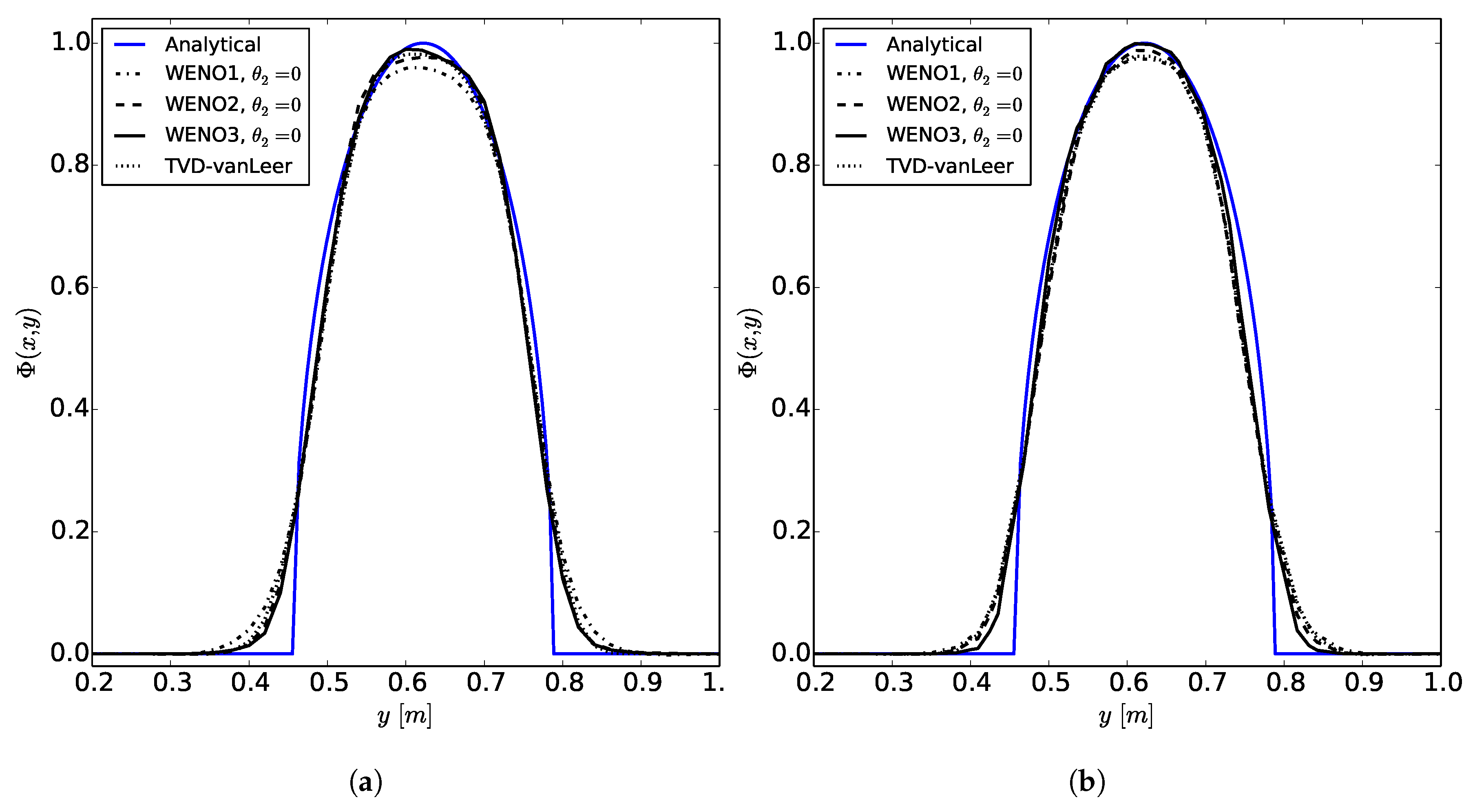
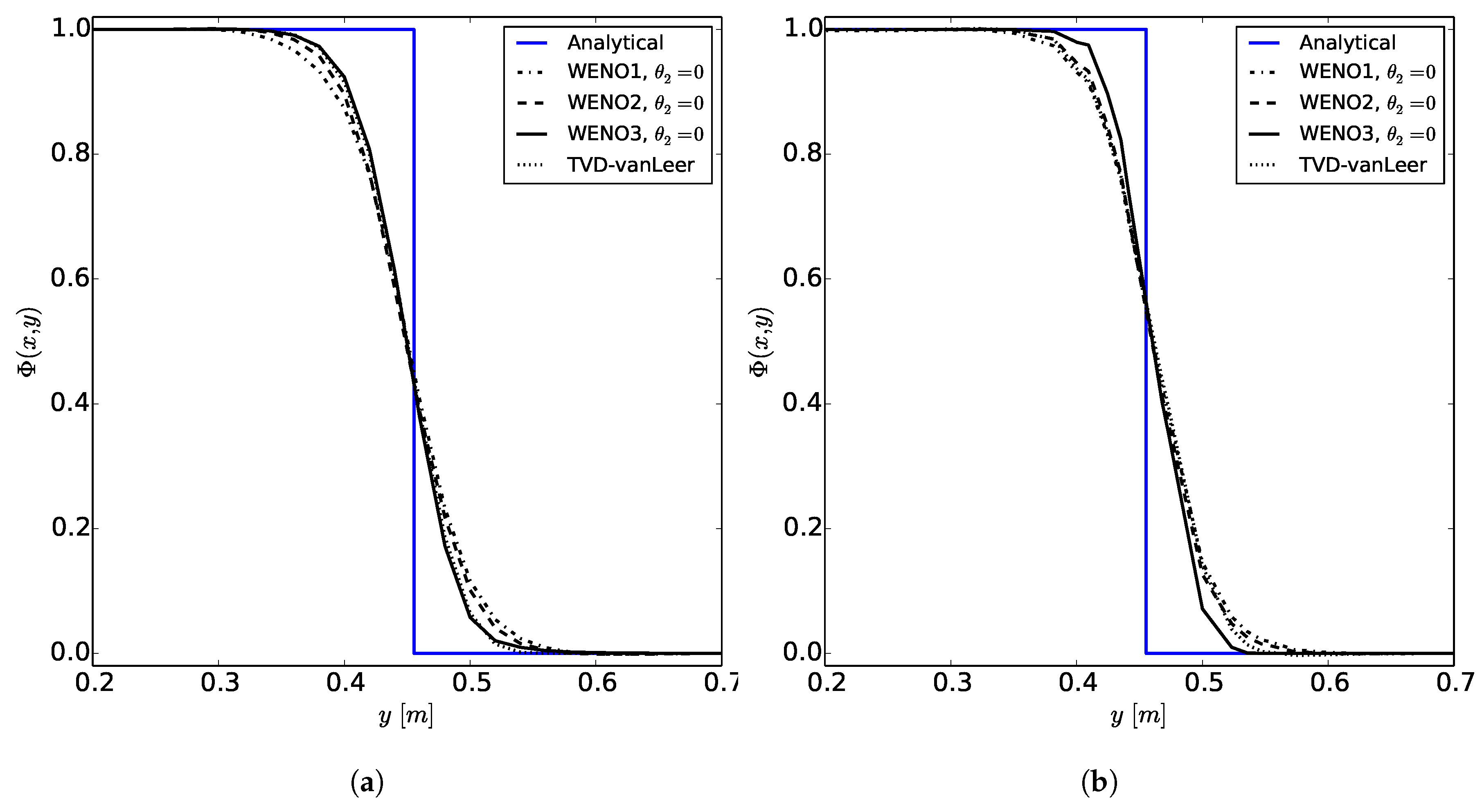
The WENOUpwindFit scheme extends the class of high-order upwind schemes and shows superior results for the scalar advection equation and in convection dominated, incompressible flows. It has been shown that the advanced handling of unstructured meshes reduces potential problems of common TVD schemes regarding accuracy and boundedness. Additionally, the stability of the simulations using the semi-implicit implementation was demonstrated. In perspective, a blending of upwind and downwind fluxes would be preferable for improving large eddy simulations or increase the accuracy of front propagating problems by avoiding MULES.

The derived gradient scheme WENOGrad represents a compromise between accuracy and efficiency, but still outperforms the standard linear gradient scheme. This class of schemes can easily be adapted to other operations in the code as the calculation of surface normal gradients (see [27] for the derivation).

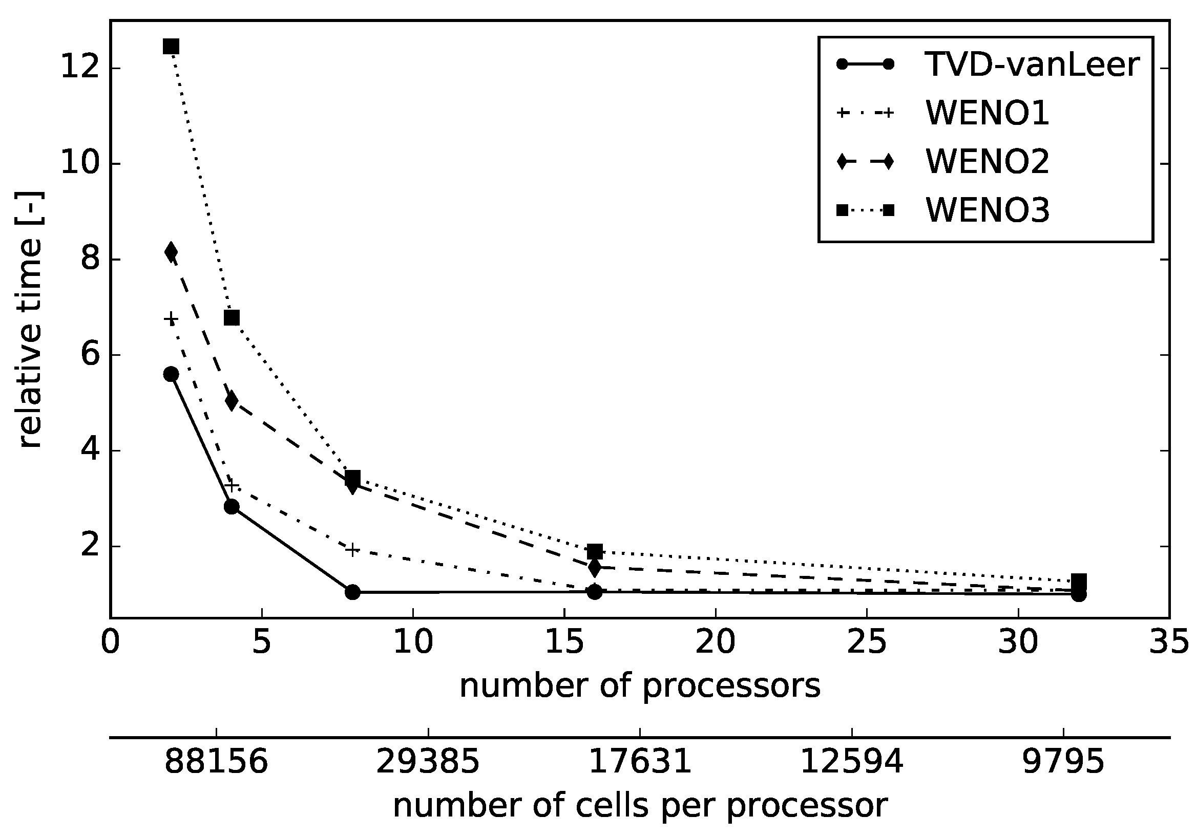
The presented efficiency analysis exposes the obvious increase at runtime during increasing the order of accuracy but also shows the possibility to reach similar computational time by increasing the number of processors. Both the preprocessing and runtime efficiency could be increased by modifying specific parameters of the reconstruction. Single test cases showed little effect of a reduced stencil expansion (compare (26)) in a reasonable range. This leads to a smaller initial stencil and less inter-processor communications in the preprocessing. The final stencil sizes are also reasonable parameters which would especially affect the runtime performance. In addition, the order of the Gaussian integration is currently fixed but could be adapted to the chosen order of the polynomials in order so save preprocessing time. Further, several approaches should be noticed which would improve the efficiency of a high-order convection scheme. The limited least-squares scheme proposed by Michalak and Ollivier-Gooch [46] is based on a single, central stencil and avoids weighting of the coefficients. The limiter could be implemented within the interpolation class similar to the presented one. Hence, the final degrees of freedom would be calculated faster than using WENO reconstructions. However, the proposed limiter is restricted to third-order of accuracy and results were just shown for the Euler equations in 2D. As an alternative approach, the adaptive WENO scheme of Costa and Don [47] might be interesting. It diminishes to a low-order upwind scheme in smooth regions and applies WENO in regions of high gradients. Thereby, a fast algorithm could be developed especially for steady-state two-phase flows where the influence of surfaces is just active in a narrow band of the domain. The difficulties are the definition of a proper criterion to distinguish between the different regions and the preservation of the accuracy of the scheme. In this connection, it is though suggested to extend the indicated performance evaluation and compute weak and strong scaling tests on the basis of a suitable benchmark test before further adjustments for performance reasons are considered.