TFF (v.4.1): A Mathematica Notebook for the Calculation of One- and Two-Neutron Stripping and Pick-Up Nuclear Reactions


1
Dipartimento di Fisica e Astronomia “G.Galilei”, Università di Padova, via Marzolo 8, I-35131 Padova, Italy
2
INFN-Sezione di Padova, via Marzolo 8, I-35131 Padova, Italy
3
Department of Physics, Faculty of Science, Karatekin University, Cankiri TR-18000, Turkey
4
Departamento de Física Atómica, Molecular y Nuclear, Facultad de Física, Universidad de Sevilla, Apartado 1065, E-41080 Sevilla, Spain
*
Author to whom correspondence should be addressed.
Computation 2017, 5(3), 36; https://doi.org/10.3390/computation5030036
Submission received: 20 July 2017
/
Revised: 27 July 2017
/
Accepted: 29 July 2017
/
Published: 3 August 2017
(This article belongs to the Section Computational Engineering)
Abstract
:The program TFF calculates stripping single-particle form factors for one-neutron transfer in prior representation with appropriate perturbative treatment of recoil. Coupled equations are then integrated along a semiclassical trajectory to obtain one- and two-neutron transfer amplitudes and probabilities within first- and second-order perturbation theory. Total and differential cross-sections are then calculated by folding with a transmission function (obtained from a phenomenological imaginary absorption potential). The program description, user instructions and examples are discussed.
1. Introduction
There is high demand for one- and two-neutron transfer reaction calculations either for planning new nuclear reaction experiments or for analyzing experimental data at energies below, above or at the Coulomb barrier as crucial tools for testing correlations in nuclear wave functions. Existing excellent broad-scope programs and tools of common use in the field of nuclear reactions (for instance, DWUCK-CHUCK [1,2], FRESCO [3], GRAZING [4], etc.) have been written with a variety of different goals, formalisms and programming languages. Our aim is not to surpass or replace those codes, but rather to offer a simple code that can be of interest to the researchers in the field of nuclear reactions, especially in connection with the renewed interest in the study of two-neutron transfer reactions with unstable nuclei. It is crucial to use transfer reactions as spectroscopic tools with halo and weakly-bound nuclei, to gain insight on pairing phenomena and pair transfer in diluted nuclear systems. The field of nuclear physics is very broad, and both nuclear structure and nuclear reaction theory have accumulated such a vast body of knowledge that some of the crucial subjects that were taken for granted only twenty or thirty years ago have mostly disappeared from the collective memory; they are too advanced to be part of basic courses in nuclear physics, and they are not easy to master. A prominent example of this phenomenon is given by neutron transfer reactions: they have been investigated quite extensively in connection with nuclei close to the stability valley [5,6], but they have been largely ‘forgotten’ by the nuclear physics community. There is at present a pressure to retrace our steps and have modern tools to meet the new demand imposed by the study of unstable nuclei. With the present notebook for Mathematica [7], we aim at covering at least one well-defined case with a simple, heavily-commented, user-friendly program that can be used without detailed knowledge of the intricacies of the mathematical formalism. Performing this kind of calculation is not an easy task; care must be taken in ensuring that many input parameters and files are properly matched, and much human intervention is needed in checking that all variables (energy, range of distances, time scales, etc.) are correctly set. This requires physical intuition and the simplicity offered by Mathematica [7] is the primary reason why we have chosen the notebook format, because it allows a closer human-machine feedback and because the flow-chart for the whole calculation can be followed and controlled, step-by-step, for each calculation in a very visual manner. The fact that parts of the calculation can be closely followed has also a didactic value. The present version of the code (v. 4.0) has been optimized and modularized for general use. Previous unpublished versions that might have circulated in private form relied on a manual feeding of input data and on unnecessary human intervention (in the calculation of for example and channel numbers) that we have now reduced to a minimum. We will assume that the user has familiarity with the notebook format and with the handling of Mathematica Kernel, with the division in cells and knows how to run them and how to interpret the syntax of functions, modules, etc.
Section 2 explains the physical scenario with reference to already published material. Section 3 explains the algorithm, the flowchart and how it is implemented. Section 4 gives practical details and instructions on how to run the code with a few examples. In the text typewriter fonts are used to express file names, variables, functions and commands, while mathematical formulas are in italics as usual.
2. Physics Background
The physical models involved in the calculations are explained in detail in the second part of [8], Chapter V. In particular, we refer to the semiclassical theory of transfer that makes use of the semiclassical coupled equations for inelastic processes (see also [9]). A number of ingredients are related either to nuclear structure, namely the modeling of the nuclei involved in the process, wavefunctions and form factors, or to the nuclear reaction, namely the description of trajectory and transfer process.
We consider a simple model for two interacting nuclei, target and projectile, in which each is described by correlated many-body states expressed in a basis generated by shell-model states. The shell-model potential is a volume Woods–Saxon with a surface spin-orbit part adjusted (depths and geometry) to reproduce some effective single-particle state. The transfer being sensitive to the tail of the wavefunction, the parameters’ adjustment must be done with the aim of obtaining the correct binding energy for each state that is included in the calculations (notice that other codes adopt drastic simplifications, such as assuming that all bound eigenstates have half the neutron separation energy). When one is considering a nucleus sufficiently close to closed shells, the single-particle wavefunctions correspond directly to the first few excited states, but when one is considering a mid-shell nucleus, the practical recipe is to obtain an effective wavefunction that has the correct quantum numbers and binding energy; although, clearly, the real correlated wavefunction is most certainly not a simple single-particle wavefunction. The program does not calculate these wavefunctions, which must be externally supplied. The file format is very general: there must be two columns of data, one for the radial variable, r, and the other for the radial wavefunction, . Any spacing in r can be used, even irregular, and the point at zero can or cannot be supplied; the program takes care of the necessary interpolations.
The two potential wells are colliding along some trajectory and with some initial bombarding energy; therefore, an ion-ion interaction is also needed to describe their relative motion. We employ two strategies: a standard Akyüz–Winther parameterization (useful when a more accurate parameterization is missing) or an optical potential with experimentally-fitted parameters. The choice between these two options, and the value of the parameters in the second case, is made in the input file. The real part of this potential, , is used to integrate the classical Hamilton–Jacobi equations of motion in the plane containing the two ions. This gives the trajectory as a function of the integration time. The imaginary part, , that is normally taken with the same geometry (although the program allows the user to make calculations even with different geometries by setting the samegeom, is used to calculate a transmission factor as a function of the impact parameter,
that will be used in the calculation of cross-sections.
Sticking to the notation of [8], we consider the following one-neutron stripping process:
where the projectile, a, is being stripped of a neutron, which is picked up by the target A. In a different notation, the reaction is . The transfer of massive particles causes a redistribution of weights between the colliding objects, and it is necessary to take into account the change of relative motion coordinates before and after the transfer (this is illustrated in Figure 4, Chapter V.4 of [8]). The coordinate system used for the evaluation of the form factors is shown in Figures 5 and 7 of the cited source.
The total Hamiltonian for the system can be written in two equivalent ways as the sum of the intrinsic Hamiltonians of the two systems plus the kinetic and potential energies of the two ions participating to the reactions, either before the transfer occurs or after, namely:
These are the so-called prior and post representations. The transfer of the neutron, from the initial state generated by the core b to the final state in core A, is caused, physically, by the fact that the tail of the neutron wavefunction in a overlaps with the potential well of the approaching reaction partner, . The mean field potential of the target nucleus A is thought to induce the transfer and in our case corresponds to the stripping of particles from a to A. If one wants to study a pick-up reaction, the role of projectile and target in the above discussion must be switched. The form factor for the transition from the channel to the channel , where Greek letters indicate collectively the configurations of the states in both projectile and target, before and after the transfer, is given by:
that is the matrix element of the initial and final channel wavefunctions and the potential that causes the transition. Under the hypothesis of single-particle states out of a core in both projectile and target, the form factors reduce to an expression involving only the single-particle wavefunctions. For the explicit calculation, we employ the formulas given in Equations (19a) and (19b) of [8], Chapter V.5.c. The form factor expression is written in a general fashion with respect to the indexes and n, but we normally use the no-recoil approximation to the lowest-order in recoil, namely we take and . The resulting expression is:
where we have applied all of the simplifications, when possible, and the coordinates refer to [8] (Figure 7, p. 323). This expression bears also the index that refers to the change in angular momentum and third component. When , one should use the symmetry relation . From Version 4.0, we have included all orders in recoil; therefore, this is no longer a limitation. From the comparison of stored form factors, one can see that the no-recoil limit represents the largest contribution.
One could simply switch to the post representation by using the substitution Equation (25) [8] (p. 333) and changing therefore the potentials to the one with index b. Although the code is written for stripping in prior representation, stripping and pickup form factors can be connected by virtue of Equations (53) and (53a) of [8] (Chapter V.5.d). In that case, post and prior representations are also swept [10].
One-neutron transfer amplitudes, for each impact parameter b, are calculated in first-order perturbation theory as:
where is the orbital integral, defined by:
for the channel . The energy of the initial and final states, and , should be given (and therefore, the reaction Q-value). Here, represents the distance in the classical trajectory, and is the azimuthal angle. The function is the phase calculated in the parabolic approximation around the point of closest approach, , as:
where and are ion-ion potentials in the entrance or exit channel, respectively, while is the velocity at the point of closest approach. The differential cross-section is:
where has already been defined, and is the probability defined for each impact parameter by:
This probability is usually taken as the probability for the transition between pure (100%) single-particle states of target and projectile. Notice that these probabilities are calculated under the hypothesis of small transfer amplitudes. At very low impact parameters, it might happen that the program calculates probabilities higher than one. This is not an error, but rather, it reflects the choice of implementing only reaction paths that go in one direction, keeping the initial flux constant. This is a valid approximation in the perturbative regime, i.e., as long as the a’s are small, and it fails when these grow too much. In any case, probabilities at these low impact parameters are folded with the transmission factor that cuts the probability distribution at about the grazing impact parameters.
The program calculates also probabilities and cross-sections for the two-neutron transfer process with :
Two-neutron transfer amplitudes are evaluated under the hypothesis of successive transfer through the intermediate states of the system () and require a second order calculation. Notice that the intermediate odd-mass nuclei correspond to b and B in the one-neutron transfer reaction above (starting from even-mass and necessarily leading to odd-mass nuclei). Clearly, and are also even. We only include the successive contribution to the amplitude that can be written as:
where the sum is extended to all of the intermediate states that are included in the coupled channel calculations. Each intermediate path is weighted with the product of two-particle spectroscopic amplitudes and , which account for the pair correlation in initial and final states with given quantum numbers. These coefficients, called occB and occb in the code, contain all needed nuclear structure information and must be externally supplied. They can be taken from shell model configurations, Hartree–Fock calculations, Bardeen-Cooper-Schrieffer (BCS)-type calculations, etc.
The one-neutron transfer reaction requires a Q-value that is calculated starting from the binding energies of the neutron with respect to the threshold in both projectile and target and the Q-value for transfer between the ground states (Q1p in the input file). The two-neutron transfer reaction requires a ground-state (g.s.) to g.s. Q-value, called Q2p, that must be supplied in the input.nb file. The coupled channel equation for the two-neutron case is solved numerically, and the results are interpolated real and imaginary parts of the transfer amplitudes (that are displayed as a function of the integration time). These are used to calculate and plot transfer probabilities, , as a function of the impact parameter. The probabilities are folded with the transmission factor (that has been calculated in the trajectory section) to obtain transfer cross-sections as a function of b as in Equation (9). One should notice the important role of the absorption factor in determining (cutting) the differential cross-section distributions at low impact parameters. There is no theoretical derivation for this parameter, which controls the depth of the imaginary potential with respect to the real ion-ion potential, and the usual practical solution is to take it close to 1/2 or 1/3. Clearly, little changes in this parameters affect the final calculations, possibly more than the little imprecision in the wavefunctions or binding energies.
Angular Distribution
With respect to preliminary versions of the code (<3.7), which were calculating cross-sections as detailed above, we have added a useful tool for experimentalists, namely the calculation of angular distributions or differential cross-section with respect to the scattering angle (). While this is a most desirable addition, the computations follow a slightly different approach and are much heavier. As a consequence, the cells that calculate them are quite slow compared to the rest (it depends of course on the number of intermediate channels that are considered). We have implemented the formalism given in [8], Chapter V. The transfer amplitudes read:
where and are the total phase shifts. The differential cross-sections are given by:
Of course, this function can be integrated in the angles, and the results match quite well (at the mb level in most cases) with the previous approach that was integrating to get the total transfer cross-section. One cannot expect a perfect match because of the numerical methods involved in the two different approaches: especially in the calculations of angular distributions, there are several oscillating contributions from all partial waves, and this forbids reaching a high level of numerical accuracy. We think that the results are nevertheless very useful to nuclear physics practitioners.
3. Flowchart Diagram and User Instructions
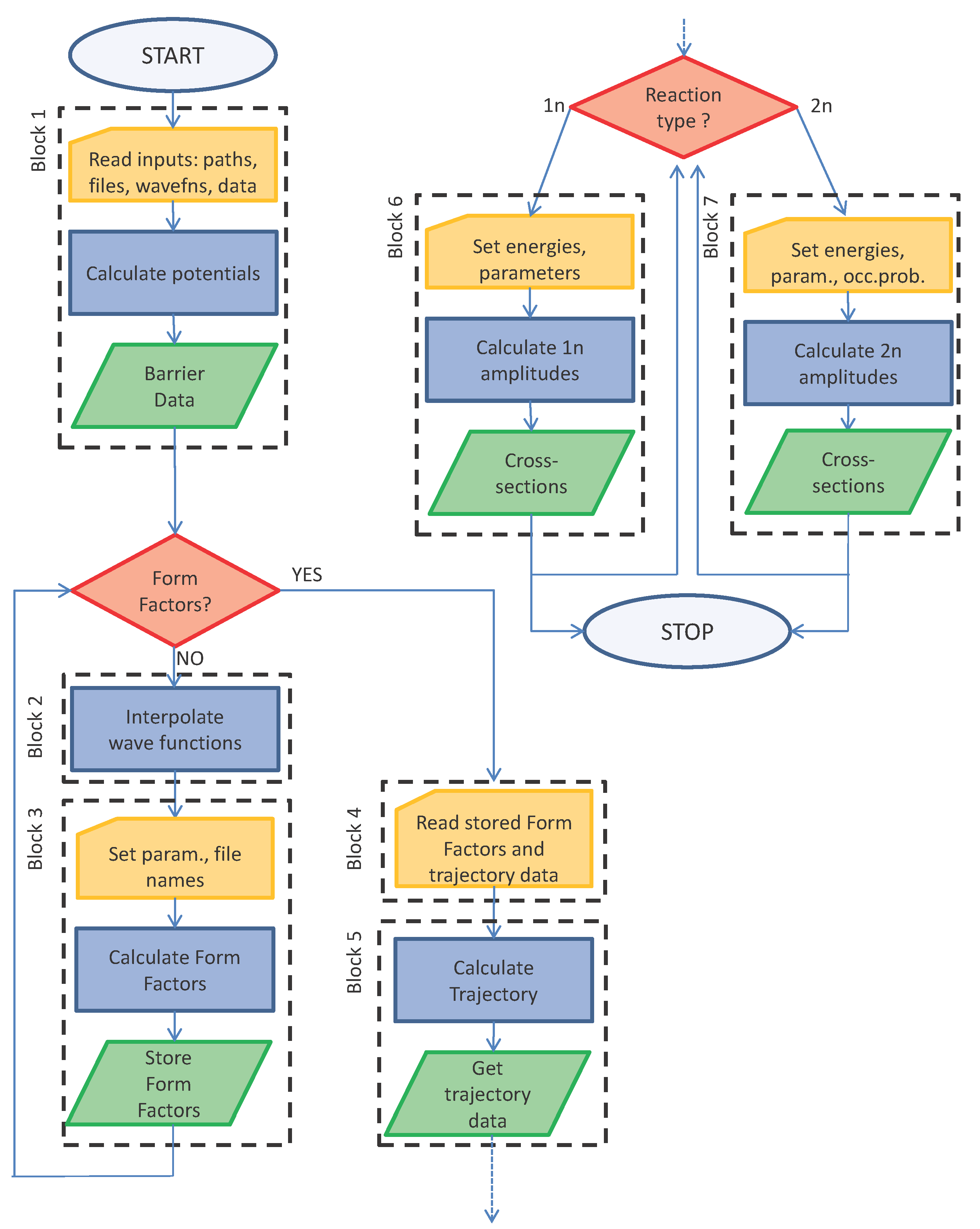
The algorithm behind the code is explained in Figure 1 with the help of a flowchart diagram. It is divided in blocks that correspond to the main groups of cells of the notebook. A few cells have lines with a yellow background: these are the input lines where data must be passed to the code. Several types of inputs are required: most of them are integers or real numbers (mostly in convenient nuclear units) that must be set case-by-case; others are strings of text (example: the path to the directory containing the files and the files’ names). Most input data are read in the file input.nb that has the Mathematica notebook format, as well. The comments and example clarify each entry.
A quick explanation of variables is given in Table 1. General specific comments about plots refer to the model examples that are given in the package.
3.1. Directories and Files
The code automatically finds the path to the directory where the notebook is saved. A working directory, wrkdir, must be specified in the first cell. We usually employ the scheme of naming the directory with the reactants of the form _, for example 208Pb_18O or 112Sn_14C, using the charges and masses of A and a in this order. This directory contains a copy of the input file called input.nb. This file can of course be renamed, and more than one file can be present in each directory because one might want, for instance, to run the code with different linear combinations of single-particle (s.p.) states, or with different absorption factors, or different potentials, etc. The input.nb file specifies which single-particle states must be used and the names of the files containing the radial wavefunctions as a function of r. These files must be stored in the Waves directory because several reactions (read different working directories) might want to access the same standard single-particle wavefunctions. Of course, by using properly-chosen labeling schemes, one can have different versions for the same single-particle state (for instance, one might want to investigate what happens if a given s.p. state is obtained from different programs or obtained at the same energy, but with different diffusivities and potential depths, etc.). We use a natural naming scheme for wavefunction files: AZz_nl(2j)%2.dat, where A is the mass number, Zz is the chemical symbol and nl(2j) are principal, orbital and total angular momentum quantum numbers. The outcomes of the calculations, i.e., form factors and differential cross-sections, are written in wrkdir. Form factors, once computed, are also read from that directory (therefore, these files should not be moved or renamed).
3.2. Block 1
The path to the directory containing input files must be set. Names of existing files should be given for the odd-mass nuclei, b and B. These files are externally supplied text files. The extension is not important as long as they are recognized as text files (we use .dat, but .txt or any other suitable extension would work, as well). These files can be read in a variety of ways, but we suggest that the wavefunction files should be set up with two columns, one for the radial variable in fm and one for the normalized wavefunction. The spacing in the radial variable is not important, nor must it necessarily be constant, because these wavefunctions are later interpolated. Next, spins, orbital and total angular momenta are read. These depend on the channel being studied and must correspond to the supplied wavefunctions. Constants are in nuclear units; masses must be given (both integers and actual masses) in atomic mass units. The potential depths used to generate the single-particle wavefunctions must be supplied in V0B and V0b. Then, the spin-orbit potential must also correspond to the potential used to generate the single-particle wavefunctions. Single-particle data are collected in a formatted table after reading the input.nb file. Notice that one can keep several different input entry files ready and just change the file name in the filetoberead string. The shell model potentials are then defined, and then, an ion-ion potential is defined following the Akyüz–Winther prescription, with an imaginary part of the same geometry: this is controlled by the absorption factor absf, usually set to 1/2. The geometry might also be altered, by setting samegeom = False, and introducing the proper values for the Akyüz–Winther parameters of the imaginary part. Alternatively, by setting akyuz = False, the ion-ion potential is taken as a generic Woods–Saxon potential, and the parameters are read from the input.nb file. The results, in terms of cross-sections, are significantly altered by small changes in the absorption because the transmission factor is folded with the probability in Blocks 6 and 7. The potential for the reactants is then plotted, and the height and position of the barrier are calculated. The ion-ion potential is also calculated for final and intermediate reaction products, because this is used in the computation of the exponents entering in the coupled channel equations.
3.3. Block 2
This step simply reads the wavefunction files and interpolates the curve. Normalization is checked, and a plot shows the overlap of data and interpolation. Notice that this step can be skipped if the form factors have already been calculated and stored (that is if ‘yes’ has already been followed at the first branching point of the flowchart). To save disk space and unnecessary duplications, we have set up the code to read wavefunctions from the Waves directory. Of course, the path to this directory can be changed, as well as the files’ names. This block (and subsequent Block 3) must be read at first run for the calculation of form factors, but can be skipped in subsequent calculations, if the form factors have been stored.
3.4. Block 3
This block calculates and stores the form factors for the chosen channel, i.e., single particle wavefunction files, quantum numbers and potentials defined in Block 1. The calculation is somewhat slow, but it needs only to be run once. Skip this block if the relevant form factors have already been calculated and stored. For each channel, this block must be run a number of times, depending on the possible values of the angular momentum transferred to the relative motion, , defined as ([8], V.4, Equation (51), p. 319, and ensuing Figure 6):
The resulting form factor is then interpolated and extrapolated to large distances with a quadratic fit model (that is checked in the plots). Normally, a linear fit should be sufficient at large distances, but we have found that a quadratic fit, with a small coefficient of the quadratic part, connects more smoothly to calculated values. It is critical that the user check every form factor (with the ListPlot, for example) and set the variable interpolationRadius to a proper value. Depending on the size of the nuclei and especially on the position of the nodes of the integrand (that somewhat reflects the nodes of the wavefunctions), we have used values of the order of 20 fm for O and Pb and up to 50 fm for more weakly-bound isotopes, the idea being that interpolationRadius is bigger than the last node, and therefore, the interpolation is made in the exponentially-decaying region. Notice that even a very tightly-bound nucleus might have a weakly-bound and broadly-extended orbital close to the threshold. The results of form factor calculations are written to conventionally-named files for each particular channel. The naming scheme used here is FF_xyz%2-xyz%2_lam = .dat, where xyz corresponds to the set of quantum numbers of the initial and final single-particle states and takes all possible values (remember that normally, the larger the , the larger the form factor value). Since the symbol / is not allowed in the file name, the %2 notation allows a straightforward reading, for example 1d3%2 or 2s1%2, etc.
See Block 7 below and Section 4 for an example.
3.5. Block 4
This block simply reads, interpolates and plots (in linear and logarithmic scales) the form factor for every channel. When inspecting the graphs, they should be free of kinks or spikes where the calculated and fitted form factors are joined. If they have these, something has gone wrong and unnoticed in the previous step. Sometimes, the fitting procedure is not working well for distances close to the interpolation radius, and a small step or kink (maybe for just one value) can be observed. This problem is usually solved by enlarging the radius at which the interpolation starts.
3.6. Block 5
Here, the reaction part starts; therefore, the user must supply further information: the laboratory bombarding energy, called Elab in the code (alternatively, the center of mass bombarding energy can be given by inverting the formula in the cell where energy is defined), the initial and final distances, rin, rf, that are usually taken as equal and large (typically 100 fm). They correspond to the disk of integration of the equations of motion. The trajectory is integrated in a time interval that goes from −tmax to +tmax, repeatedly, for a large number of different impact parameters. Some of these parameters are read in the input.nb file, and others can be adjusted in the main program itself, for example the integration time and disk radii. Notice that, for computational purposes, an integer impact parameter, m, is introduced. It has been decided that m , where b is in fm. The trajectory is solved for all up to fm. This value corresponds to mmax = 200 in the code. This value can be increased at will (at the price of slowing the calculations), for instance when one thinks that 20 fm is not enough to take into account the grazing distance if the two interacting nuclei are very large (which might happen for super-heavy or very weakly-bound orbitals). The result is a set of numerical solutions or interpolations (called Eq), labeled by m, that contain all of the trajectory information, distance, angle and conjugate momenta: , which can be evaluated and plotted. Notice that , which is connected to the total angular momentum, is a constant of motion, as it is expected for the motion in a plane. For completeness, we give also a plot of the trajectory in the reference frame.
3.7. Block 6
Here, the reaction is a one-neutron transfer, . The initial and final neutron energy with respect to the core plus neutron separation threshold must be read from the input file. This part is written in a general fashion that gives the transfer cross-section between pure single-particle configurations. Some checks are performed (might be skipped), and the system of coupled equations for the first order are solved for each and for each m in the NDSolve cell. Amplitudes are then plotted, and the probability is calculated and plotted. These plots are nonsensical at very low impact parameters, as explained above, and this region can be neglected. Based on the latter and on the transmission factor, the differential cross-section is calculated, plotted and integrated to give the total cross-section in mb . The differential cross-section can also be written to a file with the last cell.
Updates
In Version 3.7 and subsequent versions, we have added a calculation of the elastic scattering cross-section (ratio of Rutherford). This corresponds to a mere theoretical calculation obtained directly from the phase shifts (limited to a certain number of partial waves) and does not contain any folding with experimental resolution. From Version 3.9, the program can read an externally provided S-matrix in a multi-column file, called extSmat.ph, with a very generic format, namely two numbers and a string (that can also be empty), the numbers being the real and imaginary part of the S-matrix as calculated by some other program (in particular, FRESCO can be used). The phase shifts are then calculated and used instead of the one calculated in the program. This possibility must be chosen in the input file by setting the flag external = True.
3.8. Block 7
Here, the reaction is a two-neutron transfer, . The sums of squares of occupation amplitudes are calculated. Ideally, these sums should be one, though calculations can be made for partial occupations as well or for spectroscopic factors bigger than one, as is often the case from BCS calculation. Some other auxiliary functions are constructed, and form factors variables are read. Then, the NDSolve cell integrates the second order coupled equations along the trajectory to get the excitation amplitudes. This calculation might take some time depending on the number of channels and on the computer performances, but for typical case (10–20 channels), it runs in a few minutes on an Intel® Core™ i7-2640M CPU at 2.80 GHz (two cores, four logical processors) with 8 Gbytes of RAM (Windows 7 O.S.). Several amplitudes and probabilities are plotted, and a number of numerical checks is proposed. Finally, the probability is folded with the transmission factor, and the cross-sections (differential and total) are calculated and plotted. The limit of validity of the numerical subroutine that solves the coupled differential equations is very small and should not, likely, be of any practical relevance. The code gives plots of for each pair of pure (single-particle) configurations and then gives the cross-section for the special configuration given by occb and occB coefficients. Notice that the values for pure configurations are unaffected by these coefficients, and the users can change the occupation amplitudes on-the-fly in the input file, run the Input evaluation cell in Block 1 and then re-run the Cross-sect for chosen configuration cell in Block 7, without running other cells.
Updates
In Version 4.0, we have added angular distributions for the two-neutron case.
4. Model Calculations and Examples
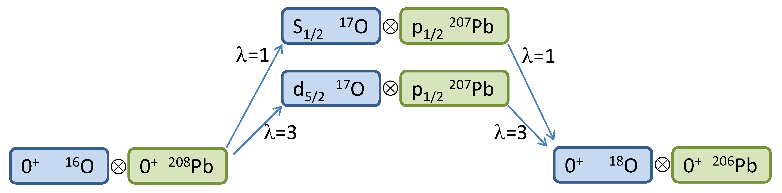
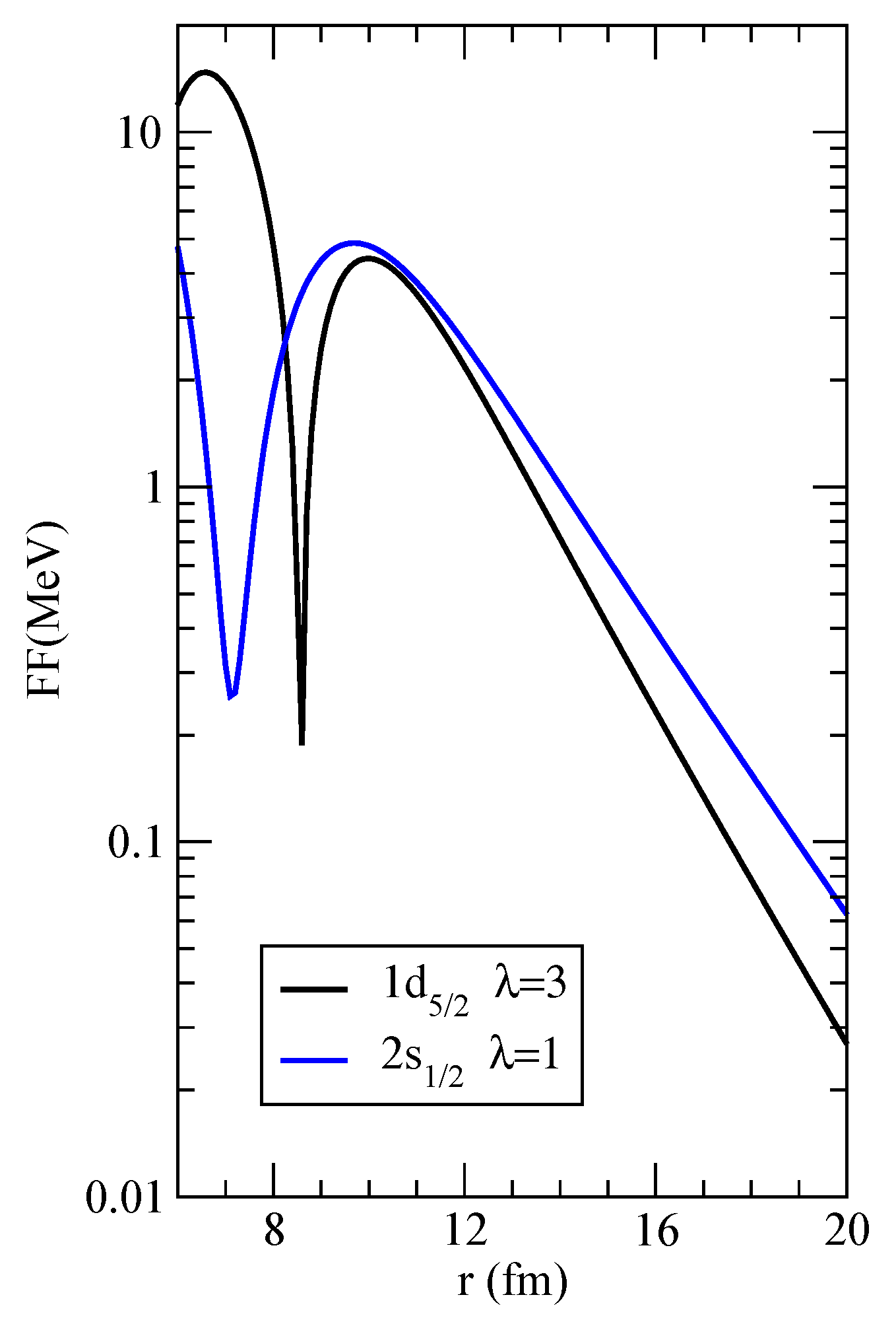
As an example, we propose the following transfer of one and two neutrons in the reactions O(Pb, Pb)O and O(Pb, Pb)O by considering only pure single-particle configurations in lead and some superposition of states in oxygen. See [11,12] for earlier studies. The wrkdir is set to be 16O_208Pb. The package comes with additional text files in the Waves directory, for the radial wavefunctions for the two nuclei, namely 17O_1d5%2.dat and 17O_2s1%2.dat, with a self-explaining naming scheme, that contain two columns of data each (r and ) for single particle wavefunctions of a neutron in the field of O and 207Pb_3p1%2.dat for the neutron hole in the ground state of Pb. In the actual Waves directory, there are also other s.p. states of lead that can be used to run more complicated cases (see below). The scheme for the two-neutron reaction with the two proposed channels is illustrated in Figure 2. Of course, this is just a very simplified model scheme; a proper calculation should entail at least the three lowest states of Pb with all possible values of , and the absorption factor should be carefully chosen in order to reproduce the data. When every variable, from paths and file names to quantum numbers and reactions parameters, is properly set, the first task is to compute and store form factors for all possible channels, which in general include not only the combinations and , but also the possible ’s. Fortunately, here is the case for a single value of in each case, and , respectively. We also furnish, as a mean of comparison, the form factors for these two channels in the files FF_1d5%2-3p1%2_lam=3.dat and FF_2s1%2-3p1%2_lam=1.dat. The former is plotted in logarithmic scale in Figure 3. This information can be used to check Blocks 1–3 along the flowchart of Figure 1.
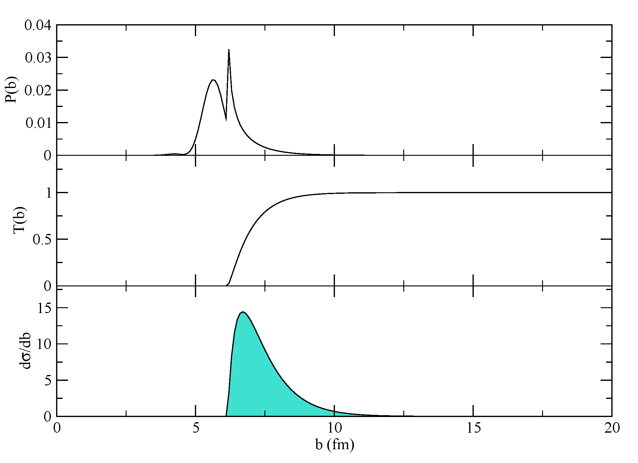
We set the variable Elab, which is the bombarding energy in the laboratory frame, to MeV (which corresponds to ∼40% above the barrier). This energy for the lead beam has been chosen to match the laboratory energy of the O beam of 104 MeV of [13] in order to allow for a simple order of magnitude check. They both give a center of mass energy of MeV. One can then run Blocks 1, 4, 5, 6 or 1, 4, 5 and 7: this corresponds to following the answer yes at the first decisional branching point of Figure 1 and then deciding between one- or two-neutron transfer (or both) at the second branching point. Block 2 is not mandatory. Notice that Blocks 2 and 3 are optional or unnecessary because the form factors have already been calculated. Of course, one can also run Blocks 1, 4–7 in a single calculation. The outcome of the calculations can be written to a file, and it is illustrated in Figure 4 where the transfer probability, the transmission factor and the resulting cross-section are displayed for a typical case. The effect of the absorption, which cuts the innermost part of the probability, is very important in determining the total cross-section, because this is changing quickly around the grazing region. The final integrated cross-sections are given in mb for the one- and two-neutron transfers, respectively. A proper modeling of the reaction should include an adjustment of the absorptive part of the potential according to the discussion in [8] (Chapter V, Section 7). Not only the depth, but also the geometry of the imaginary part of the potential should be adjusted to match the experimental findings at different bombarding energies. If the program runs correctly, it should give, for the two channels, 9.74161 mb and 24.4565 mb in the 1n-transfer reaction and 0.0420219 mb and 0.669721 mb for the 2n-transfer reaction (for pure configurations of oxygen). The actual configuration of oxygen, , with the for lead (with occb[1] = 1), should give 0.267993 mb. Clearly, these numbers do not perfectly match the published data in [13], because there has been no detailed search on the optimal modeling of potentials, wavefunctions, ion-ion interaction, absorption factors, and so on. In fact, it is probably necessary to reduce the absorption factor to about 1/3 and adjust the potentials’ geometry to match the root mean square radii. Notice that the input file contains three states for lead, but the parameter nstb has been set to one, so that only the g.s. is read. The reader might want to set it to three and run the code in order to see a more complicated case. If everything has run properly, taking all spectroscopic amplitudes equal to unity for simplicity, the final outcome should be mb.
We have used preliminary versions of this code to generate the calculations used in [14] for the reactions Sn (C,C) Sn, Sn (C,C) Sn, Mg (O,O) Mg and Ni (C,C) Ni.
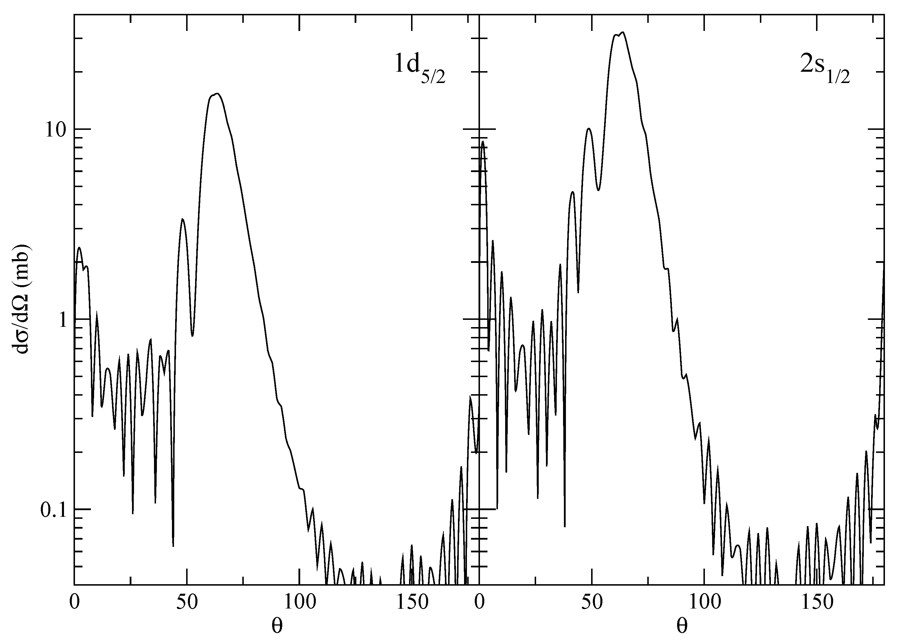
The supplementary calculations for the angular distributions (see Figure 5) are run within the cell (they can be skipped).
4.1. Practical Suggestions
After inserting the chosen masses and charges for the reaction participants, the program displays the reaction in the Block 1, input evaluation cell, which can be used to check the correctness of data. Keep in mind that the numbers found in the first two columns of the channels cell refer to the sequence in which the data are written in the input.nb file; there is no re-ordering or sorting of any type. The channel’s numbers (for the particular configuration) simply count the different ’s in ascending order. These numbers are useful when the reaction calculations are performed in Blocks 6 and 7, and the user should return to this table for the interpretation of the results. It is often useful to know the Coulomb barrier height before choosing a laboratory or center of mass energy in the input file: one could run Block 1 with a dummy energy datum, inspect the barrier height from the plot potentials cell, correct and save the input.nb file and then run again the input evaluation cell. Always remember to inspect the bombarding energy that is given in the trajectory parameters, auxiliary functions cell in Block 5. The Example cells in Blocks 6 and 7 run with all entries for channels equal to one, because this ensures that they will always run. Of course, the user might want to check another channel and a different impact parameter (remember that m is ten times b). In these cells, for simplicity.
4.2. Operating Systems
The way in which the software expresses the paths to the files to be loaded might be dependent on the particular operating system (OS). Users might experience some difficulties when trying to load files. We have not tested our notebook on an OS different from Windows 7, and we are not aware of any special problem related to OS-dependent paths. Therefore, the most practical solution is to change the cells that refer to paths according to the rules of the users’ OS. For example, Windows uses the double backslash, , to separate directories, while Linux/Unix uses a single slash symbol, /.
5. Conclusions and Warnings
The formalism for transfer is a most complex topic and should be treated with care [15]. The approach that has been implemented in the present code entails a number of approximations (no-recoil, prior/post) in the calculation of the form factors, and it is based on a semiclassical trajectory formalism. The cross-section is therefore strongly dependent on the absorption parameter that has a phenomenological nature. Nevertheless, it can be useful to estimate the order of magnitude cross-sections for planning experiments, and the possibility to use arbitrary mixtures of single-particle states in both target and projectile allows for a broad category of studies on the effects of pairing correlations in transfer reactions. A word of caution should also be issued: changing reaction parameters, like masses, charges, bombarding energies, etc., must be accompanied by a careful check of the trajectory integration, namely the time that the ion takes to traverse the integration disk (whose radius has been set in the variable rin). It might be the case that at high energies, the velocity is quite high, and there is no time for multiple interactions between target and projectile (in that case, one should try and reduce the time steps). Another possibility is the appearance of orbiting phenomena, for a certain given impact parameter, which are usually quite small and tend to be washed out by the transmission factor distribution. To keep this under control, the cell trajectory integration in Block 5 plots the time of closest approach as a function of the impact parameter: a cusp behavior might mark an incomplete orbiting. Each case must be examined anew, and a proper check of the subroutine that solves the coupled differential equation should be performed by inspecting the outcome of the integration.
Before publication, several other trials have been made with various reactions, obtaining sensible results in practically all cases. Sometimes, we had to adjust the absorption factor (the most extreme cases being 0.25 and 0.65) to get order of magnitude estimates. Even if this adjustment is a necessary step, the code is useful to understand the percentage of s.p. components that enters into a certain configuration or to exclude the negligible components, and so on. It allows a deeper understanding of the detailed structure and permits making a statement about the relative weights of various competing reaction paths. The angular distributions do not always match experimental data; often, the secondary peaks (on the two sides of the grazing peak) show an increased oscillatory pattern, while the data are smoother: one intrinsic reason is that the formalism produces pure diffraction patterns that might be blurred in the experiment due to the experimental angular resolution of the detectors; another reason is that the particular implementation allows a finite number of differential equations to be solved/integrated simultaneously, while the formalism would converge ideally only with full summations. The area close to the grazing angle (the one that matters most) is most always correctly reproduced.
5.1. Approximations and Limitations
In addition to what has been said in the previous section, we want to highlight a few additional points that illustrate the connections between approximations and the limitations that they introduce.
5.1.1. No Recoil
This has been discussed in Section 2. Up to Version 3.9 only, was included, but now, the form factors are calculated with an appropriate treatment of recoil. Ideally, one should not use this formalism for transfer in light ions. At the same time, the bombarding energies should be kept low.
5.1.2. Semiclassical Trajectories
In principle, the Coulomb interaction acts over an infinite range; therefore, each integration of the trajectories on a disk of finite size is subject to some error. We think that in our scheme, this is under control and can be made more accurate, if necessary, by acting on the variable rin.
5.1.3. Sequential 2n Transfer
This has to do with the nature of the residual pairing interaction among the valence neutrons. In the independent particle limit, the non-orthogonal and simultaneous contribution to the transfer amplitudes cancel each other, and this is the limit in which we operate, taking into account all of the intermediate paths that might lead to the final states. If strong correlations are present, one might invoke simultaneous transfer of a dineutron as the favored reaction mechanism, and another code should be used.
5.1.4. No Coupling to Other Channels
One might encounter the situation in which coupling to other channels can be expected (this depends on the energy above/below Coulomb barrier and on the details of the nuclear structure of target and projectile). For example, if strong transitions to states are present, one might need to include additional couplings as in standard coupled-channels Born approximation codes.
5.2. Work Plan for Future
We are working on a database of standard wave functions and form factors for transfer reactions with stable and unstable nuclei with the aim of providing guidance in the planning of future experiments. From a more theoretical point of view, one could start studying what happens when reactions are carried out with halo states (by repeating calculations with various wave functions) or what happens when one reaches the drip-line, and so on.
Supplementary Materials
The following are available online at https://www.mdpi.com/2079-3197/5/3/36/s1; Sample: All of the TFF (v.4.1) codes.
Acknowledgments
We acknowledge funds granted by the University of Padova (Italy) and by the INFN-Section of Padova (Italy). In particular, J.-A. Lay acknowledges funding from the Marie Curie-Piscopia fellowship program of the University of Padova.
Author Contributions
All authors, at different times while working for the University of Padova and the INFN -Section of Padova, have contributed to the program writing, debugging and testing. In particular, A. Vitturi and I. Inci started the core of the form factor calculations (Code Block 3). L. Fortunato has written the other blocks with help from A. Vitturi and J.-A. Lay in Blocks 1, 6 and 7. J.-A. Lay has made several tests and added several options.
Conflicts of Interest
The authors declare no conflict of interest.
References
- Kunz, P.D. Instructions for the Use of Dwuck, a Distorted Wave Born Approximation Program; Technical Report, COO-535-606; Colorado University Boulder Department of Physics: Boulder, CO, USA, 1969. [Google Scholar]
- Kunz, P.D. Algebra Used by Dwuck with Applications to the Normalization of Typical Reactions; Technical Report, COO-535-613; Colorado University Boulder Department of Physics: Boulder, CO, USA, 1970. [Google Scholar]
- Thompson, I.J. Getting started with FRESCO. Comput. Phys. Rep. 1988, 7, 167–212. [Google Scholar] [CrossRef]
- Pollarolo, G.; Winther, A. Program GRAZING_9 A Fortran Program for Estimating Reactions in Collision between Heavy Nuclei. 2000. Available online: http://personalpages.to.infn.it/~nanni/grazing/ (accessed on 17 January 2017).
- Bayman, B.F.; Chen, J. One-step and two-step contributions to two-nucleon transfer reactions. Phys. Rev. C 1982, 26, 1509–1520. [Google Scholar] [CrossRef]
- Maglione, E.; Pollarolo, G.; Vitturi, A.; Broglia, R.A.; Winther, A. Absolute cross sections of two-nucleon transfer reactions induced by heavy ions. Phys. Lett. B 1985, 162, 59–65. [Google Scholar] [CrossRef]
- Mathematica, version 8; Wolfram Research, Inc.: Champaign, IL, USA, 2010.
- Broglia, R.A.; Winter, A. Heavy Ion Reactions: Parts 1 and 2; Addison-Wesley Publishing Co.: Harlow, UK, 1991. [Google Scholar]
- Alder, K.; Winther, A. Electromagnetic Excitation: Theory of Coulomb Excitation with Heavy Ions; North-Holland Publishing Co.: Amsterdam, The Netherlands, 1975. [Google Scholar]
- Broglia, R.A.; Liotta, R.; Nilsson, B.S.; Winter, A. Formfactors for one-and two-nucleon transfer reactions induced by light and heavy ions. Phys. Rep. 1977, 29, 291–362. [Google Scholar] [CrossRef]
- Dasso, C.H.; Vitturi, A. Collective Aspects in Pair-Transfer Phenomena; Società Italiana di Fisica Editrice Compositori: Bologna, Italy, 1988. [Google Scholar]
- Dasso, C.H.; Pollarolo, G.; Landowne, S. On the imaginary part of the form factor for inelastic excitations in heavy-ion reactions. Nucl. Phys. A 1985, 443, 365–379. [Google Scholar] [CrossRef]
- Pieper, S.C.; Macfarlane, M.H.; Gloeckner, D.H.; Kovar, D.G.; Becchetti, F.D.; Harvey, B.G.; Hendrie, D.L.; Homeyer, H.; Mahoney, J.; Pühlhofer, F.; et al. Energy dependence of elastic scattering and one-nucleon transfer reactions induced by 16O on 208Pb. I. Phys. Rev. C 1978, 18, 180–204. [Google Scholar] [CrossRef]
- Lay, J.A.; Fortunato, L.; Vitturi, A. Investigating nuclear pairing correlations via microscopic two-particle transfer reactions: The cases of 112Sn, 32Mg, and 68Ni. Phys. Rev. C 2014, 89, 034618. [Google Scholar] [CrossRef]
- Thompson, I.J. Reaction mechanisms of pair transfer. arXiv, 2013; arXiv:1204.3054v2. [Google Scholar]
Figure 1.
Flowchart diagram of the code. Blocks (corresponding to groups of cells) are indicated with dashed black boxes. Inside each block, data reading is indicated as yellow cards, algorithms are indicated as blue rectangles and outputs as green parallelograms. Red rhombi define decisional branching points. Notice that Blocks 2 and 3 can be skipped when form factors are already known (i.e., when Block 2 plus Block 3 have been successfully run in a previous calculation).

Figure 2.
Scheme of channels for the example reactionO(Pb, Pb)O. Only two states of oxygen are used for the sake of simplicity. More accurate schemes must contain all relevant single-particle states in both target and projectile and, for each combination, all possible values of .
Figure 2.
Scheme of channels for the example reactionO(Pb, Pb)O. Only two states of oxygen are used for the sake of simplicity. More accurate schemes must contain all relevant single-particle states in both target and projectile and, for each combination, all possible values of .

Figure 3.
Form factor for the and transfers with and 1 respectively as a function of the ion-ion distance r.
Figure 3.
Form factor for the and transfers with and 1 respectively as a function of the ion-ion distance r.

Figure 4.
Transfer probability, transmission factor and the resulting differential cross-section () are displayed as a function of the impact parameter b for a typical case. Small changes in the imaginary potential affect the transmission factor and consequently the cross-section profile of the lower panel. The present simplified example does not refer to the case discussed in Section 4.

Figure 5.
Angular distribution () as a function of the angle for the two states of O considered in the paper. This has been obtained with the parameters I3 of [13]. The small mismatch with respect to the results obtained there can be attributed to small differences in the code and can be easily fixed with small adjustments in the parameters.

Table 1.
Summary of user-defined variables. If the index i is present, it refers to the particular state from 1 to nstB or nstb. Target and projectile are referred to with B and b, while c labels the channel.
Table 1.
Summary of user-defined variables. If the index i is present, it refers to the particular state from 1 to nstB or nstb. Target and projectile are referred to with B and b, while c labels the channel.
| Code Variables | Explanation | Units or Values |
|---|---|---|
| mA, ma, mB, mb | Mass | amu |
| AA, Aa, AB, Ab | Mass number | - |
| ZA, Za, ZB, Zb | Atomic numbers | - |
| lB[i], lb[i] | Orbital angular momentum of B, b | - |
| jB[i], jb[i] | Total angular momentum of B, b | - |
| sB[i], sb[i] | Spin of single-particle in B, b | 1/2 |
| V0A[i],V0b[i] | Potential depth (volume) in B and b | MeV |
| VlsB[i],Vlsb[i] | Spin-orbit potential depth (surface)) in B, b | MeV |
| a | Diffusivity | fm |
| absf | Absorption factor | 0.5 (typically)) |
| akyuz | Select Akyuz-Winther or optical pot. | False/True |
| samegoem | Select equal geometry for W and V | False/True |
| external | Select external phase shifts | False/True |
| interpolationRadius | Interpolation radius | fm |
| Angular momentum transfer | - | |
| Order of recoil power expansion | 0 | |
| En | Center of Mass bombarding energy | MeV |
| rin | radius of integration disk | fm |
| rffmin, rffmax | Form factors range of r | fm |
| tmax | ‘Asymptotic’ time | fm/c |
| m, (mm, mdum) | Integer impact parameter, | fm/10 |
| EB[i], Eb[i] | Neutron binding energies | MeV |
| SpecB[i], Specb[i] | Single particle energies above the g.s. | MeV |
| Q1p | Q-value for one-neutron transfer | MeV |
| Q2p | Q-value for two-neutron transfer | MeV |
| occB[i], occb[i] | Occupation amplitudes | - |
| chn[B,b] | Channel number | |
| [B,b,c] | Angular momentum transfer of channel c | - |
| howmany | Number of channels | - |
© 2017 by the authors. Licensee MDPI, Basel, Switzerland. This article is an open access article distributed under the terms and conditions of the Creative Commons Attribution (CC BY) license (http://creativecommons.org/licenses/by/4.0/).
Share and Cite
MDPI and ACS Style
Fortunato, L.; Inci, I.; Lay, J.-A.; Vitturi, A. TFF (v.4.1): A Mathematica Notebook for the Calculation of One- and Two-Neutron Stripping and Pick-Up Nuclear Reactions. Computation 2017, 5, 36. https://doi.org/10.3390/computation5030036
AMA Style
Fortunato L, Inci I, Lay J-A, Vitturi A. TFF (v.4.1): A Mathematica Notebook for the Calculation of One- and Two-Neutron Stripping and Pick-Up Nuclear Reactions. Computation. 2017; 5(3):36. https://doi.org/10.3390/computation5030036
Chicago/Turabian StyleFortunato, Lorenzo, Ilyas Inci, José-Antonio Lay, and Andrea Vitturi. 2017. "TFF (v.4.1): A Mathematica Notebook for the Calculation of One- and Two-Neutron Stripping and Pick-Up Nuclear Reactions" Computation 5, no. 3: 36. https://doi.org/10.3390/computation5030036
Note that from the first issue of 2016, this journal uses article numbers instead of page numbers. See further details here.