DiamondTorre Algorithm for High-Performance Wave Modeling

Abstract

Effective algorithms of physical media numerical modeling problems’ solution are discussed. The computation rate of such problems is limited by memory bandwidth if implemented with traditional algorithms. The numerical solution of the wave equation is considered. A finite difference scheme with a cross stencil and a high order of approximation is used. The DiamondTorre algorithm is constructed, with regard to the specifics of the GPGPU’s (general purpose graphical processing unit) memory hierarchy and parallelism. The advantages of these algorithms are a high level of data localization, as well as the property of asynchrony, which allows one to effectively utilize all levels of GPGPU parallelism. The computational intensity of the algorithm is greater than the one for the best traditional algorithms with stepwise synchronization. As a consequence, it becomes possible to overcome the above-mentioned limitation. The algorithm is implemented with CUDA. For the scheme with the second order of approximation, the calculation performance of 50 billion cells per second is achieved. This exceeds the result of the best traditional algorithm by a factor of five.

1. Introduction

Among the issues of contemporary stencil computations, we find the following two to be the most prominent.

The first issue is the inability to operate on all levels of parallelism with maximum efficiency. It may be solved for some software (testing packages like LAPACK [1] being the evident example), but remains an open question for the larger part of relevant problems. Furthermore, to achieve this, it is necessary to use several programming instruments. As the supercomputer performance is mostly increased by adding levels of parallelism, the modern top 500 computers [2] are essentially heterogeneous, and the majority of them include the GPGPU. The peak performance is achieved by using all levels of parallelism in some ideal way. The sad truth about the expensive supercomputers is that they mostly run software that does not accomplish this requirement. To efficiently utilize the supercomputing power, the software should be written with regard to the model of the parallelism of a given system.

For physical media simulation, the common method of utilizing concurrency is domain decomposition [3]. It assumes decomposition into large domains, the data of which fit into the memory attached to a processor (coarse-grained parallelism). The common technology to implement this is MPI [4].

The other method, tiling [5], is often used in computer graphics and other applications. The data array is decomposed into small parts, which all lie in the same address space (fine-grained parallelism), and OpenCL [6] and CUDA [7] are common technologies for this. A similar technique is loop nest optimization [8]. It appears when initially sequential programs are rewritten to be parallel and a dependency graph [9] has to be analyzed to find an optimal algorithm. It is often executed with OpenMP [10] in coarse-grained parallelism and loop auto-vectorization [11] in fine-grained parallelism. With all parallel technologies, developers have to struggle with the issues of unbalance, large communication latency and low throughput, non-uniform data access [12] and necessity of memory coalescing [7].

The second issue in applied computations that deal with processing large amounts of data (such as wave modeling) is the deficiency in memory bandwidth. The balance of main memory bandwidth to peak computation performance is below 0.1 bytes/flop for the majority of modern computers and tends to decrease even further as new computation units appear. In terms of hardware, the access to data takes more time and costs more (in terms of energy consumption) than the computation itself.

Our aim was to construct an algorithm to solve these issues for stencil computations for GPU-based systems. It should naturally utilize all available levels of parallelism and efficiently work with all levels of the memory hierarchy. A decomposition of the modeling domain in both time and space was essential to achieve this aim. Such an approach was used before by other authors [5,13,14,15,16,17], but the mentioned problems of the incomplete use of parallel levels and memory layers have not been sufficiently solved. Further, we aim to develop a theoretical model for an a priori assessment of the performance efficiency by combining the knowledge of the computer system, the numerical scheme and algorithm characteristics. The algorithm is implemented with CUDA, since it is an instrument that allows convenient use of GPU parallelism and memory hierarchy levels [18,19] .

2. Computation Models

With the hierarchy of memory subsystems and levels of parallelism, contemporary computers display an extreme complexity.

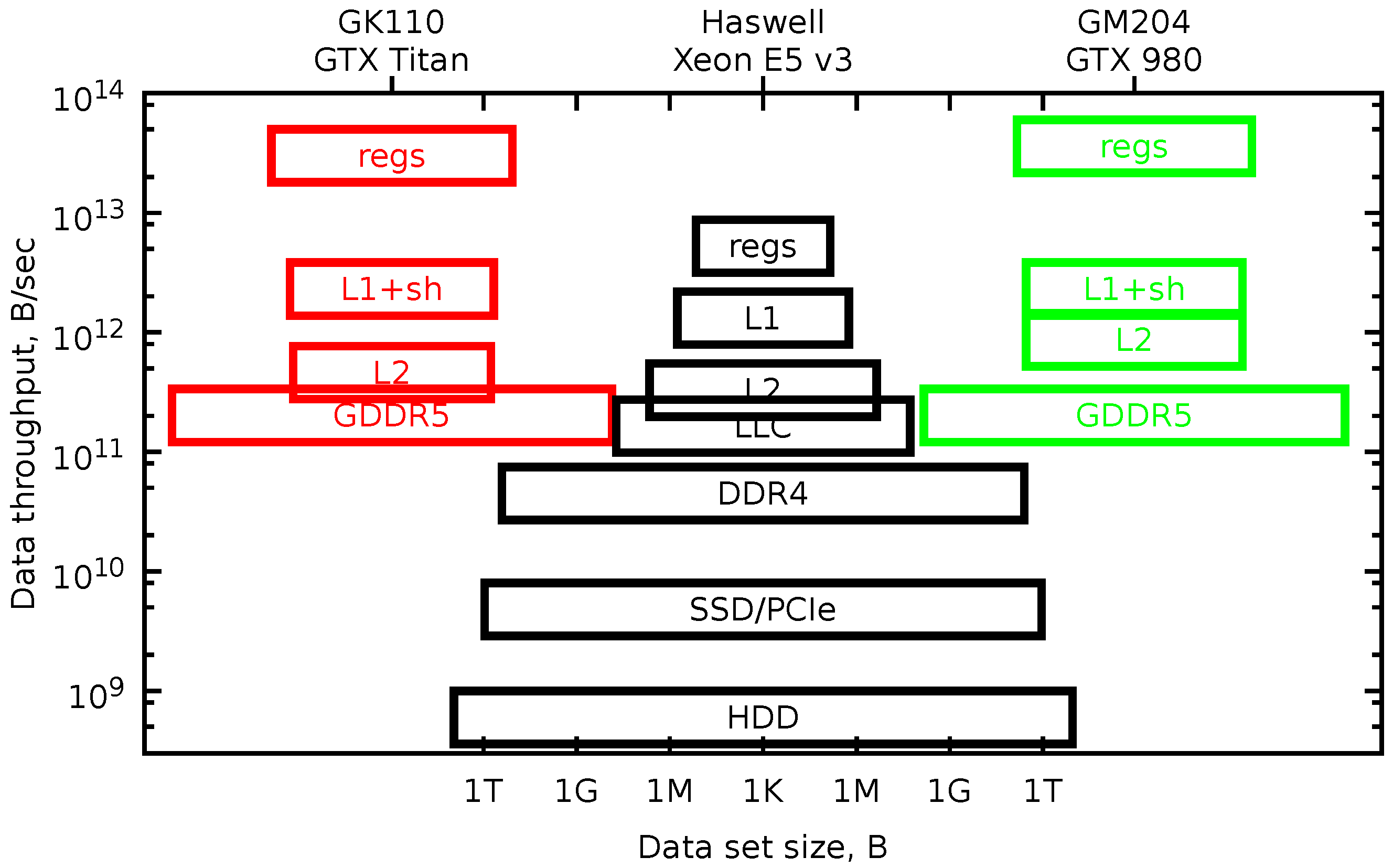
One helpful tool is a model of the pyramidal memory subsystem hierarchy. In Figure 1 in a log-log scale, we plot rectangles, the vertical position of which shows the data throughput of the memory level, and the width of the rectangle shows the dataset size. The picture looks like a pyramid for the CPU device. With each level, the memory bandwidth is about twice higher, and the data size is smaller by a factor of eight.

Locally-recursive non-locally-asynchronous (LRnLA) algorithms [20,21] use the divide and conquer approach by decomposing the problem into subproblems recursively at several levels, so that each time, the data of the subproblems fit into a higher level of the memory hierarchy. It allows one to reach peak performance for the problems, the data of which are as large as the lower level of the memory subsystem.

This idea of recursive subdivision has been implemented in the LRnLA algorithm ConeFold. It has provided the expected performance increase for CPU-based codes [21].

The register memory of GPGPU is larger than the CPU cash, so it may be used as a main data localization site. This register file is distributed between several multiprocessors. The next significant memory level (GDDR5) has worse memory bandwidth and latency. Therefore, instead of recursive decomposition, it is important to provide a continuous data flow from device memory to registers and back.

The DiamondTorre LRnLA algorithm has been developed based on this idea [22,23,24]. In this paper, we show how it is constructed, discuss its characteristics, provide CUDA implementation details and show its performance results on a simple memory-bound stencil problem. This paper is focused on performance optimization for one device.

The hierarchy is best known to hardware designers, but this knowledge is impossible to ignore in the programming process. The complex computer structure should be simplified as some model. One example of such a model is the roof line. Introduced in [25], the roof line model is a graph of attainable GFlops per second versus operational intensity. It has two distinct portions and visually assorts the programs into the two categories based on the operational intensity: memory bound and compute bound. The higher the ceiling rises (this corresponds to the increase in peak performance), the more problems fall under the slope and suffer from memory bandwidth limitations.

3. Problem Statement

The main scope of the current work is the wave modeling, which encompasses a vast range of applications, such as the modeling of: elastic media wave propagation, nanophotonics, plasmonics and acoustics. To be specific in the present paper, we choose to limit the discussion to the acoustic wave equation, but the implications are easily generalized to all numerical methods with a local stencil.

$$\frac{{\partial }^{2}F}{\partial t^2}=c^2\left(\frac{{\partial }^{2}F}{\partial x^2}+\frac{{\partial }^{2}F}{\partial y^2}+\frac{{\partial }^{2}F}{\partial z^2}\right)$$

(1)

The problem is to compute the temporal evolution of a field $F=F(x,y,z,t)$ in a finite simulation domain with the given initial ($F(x,y,z,0)=F_0(x,y,z)$) and boundary (${F|}_{boundary}=U\left(t\right)$) conditions. The explicit scheme has the second order of approximation in time and an adjustable order of approximation in space. That is, the mesh is introduced over the domain with $Nx$, $Ny$, $Nz$ cells along each axis, and the differentials are approximated by the finite sums of the form:

$${\Delta }{x}^2{\left.\frac{{\partial }^{2}F}{\partial x^2}\right|}_{x_0,y_0,z_0,t_0}=\sum _{i=0}^{N_O/2}{C}_i{\left(F\right|}_{x_0+i{\Delta }x}+F{|}_{x_0-i{\Delta }x})$$

(2)

where $N_O$ is the order of approximation (it is even), $C_i$ are the numerical constants (sample coefficients are given in the

Table 1. Numerical scheme coefficients.

${\mathit{N}}_{\mathit{O}}$	${\mathit{C}}_{\mathbf{0}}$	${\mathit{C}}_{\mathbf{1}}$	${\mathit{C}}_{\mathbf{2}}$	${\mathit{C}}_{\mathbf{3}}$	${\mathit{C}}_{\mathbf{4}}$
2	$-1$	1	—	—	—
4	$-5/4$	$4/3$	$-1/12$	—	—
6	$-49/36$	$3/2$	$-3/20$	$1/90$	—
8	$-205/144$	$8/5$	$-1/5$	$8/315$	$-1/560$

) and Δ signifies a mesh step along the corresponding axis. Differentials in all four variables are expressed similarly. $N_O=2$ for the time derivative; $N_O=2,4,6...$ and more for space derivatives.

The following computation should be carried out to propagate the field value to a new ($k+1$)-th time layer:

$${F|}^{k+1}=2F{{|}^k-F|}^{k-1}+c^2{\Delta }{t}^2\left({\left.\frac{{\partial }^{2}F}{\partial x^2}\right|}^k+{\left.\frac{{\partial }^{2}F}{\partial y^2}\right|}^k+{\left.\frac{{\partial }^{2}F}{\partial z^2}\right|}^k\right)$$

(3)

assuming that all values on the right-hand side are known. In the implementation, the field data for two sequential time layers should be stored. Thus, it is common to use two program arrays F and G: one for the even time steps, another for the odd ones. To compute, it is necessary for $2+3N_O$ values to be loaded from memory, one to be saved to memory, and if values like $c^2{\Delta }{t}^2/{\Delta }{x}^2$ are defined as constant, the number of FMA (fused multiply-add) operations in the computation is at least $1+3N_O$.

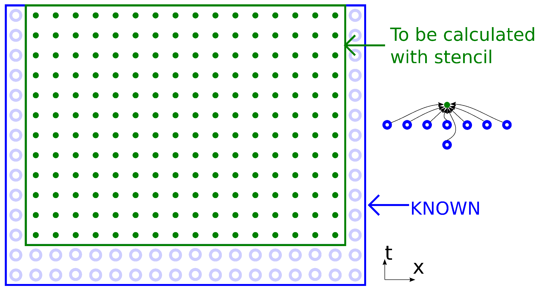
By applying the stencil for each point in the $(d+1)$-dimensional mesh (d coordinate axes and and one time iteration axis), we get an entity that we will call a “dependency graph” in this paper (Figure 2). The first two layers along the time axis are an initial condition; the last layer is the desired result of the modeling problem. Between layers, the directed edges show the data dependencies of the calculations, and calculations are represented by vertices (the top point of the stencil that corresponds to ${F|}^{k+1}$). Initial values and boundary points represent the initialization of a value instead of calculation with a stencil. All stencil computations in the graph should be carried out in some particular order.

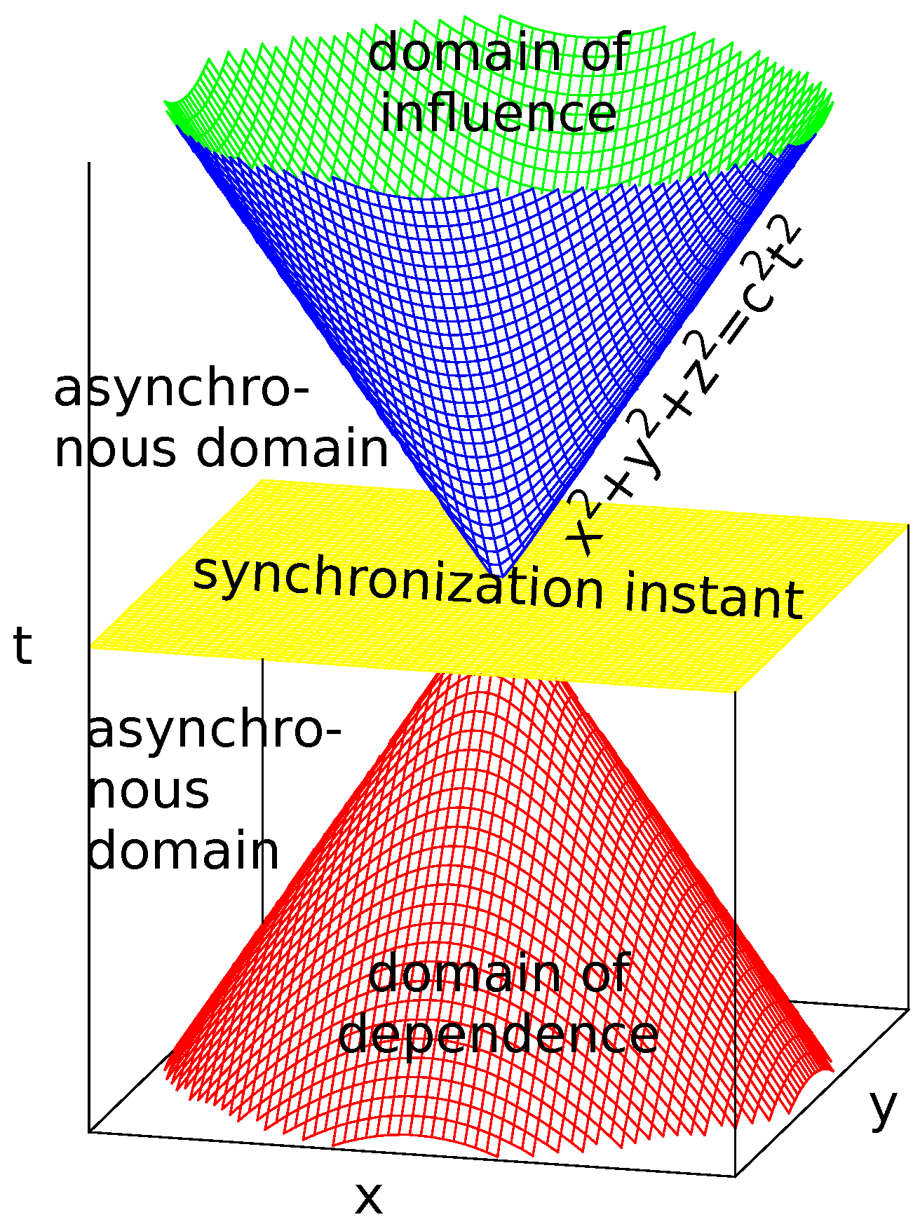
The inherent property of the physical statement of the problem is a finite propagation velocity. According to the special relativity, there exists a light cone in 4D spacetime, which illustrates the causalities of events (see Figure 3). For a given observer spot, all events that affect it are contained in a past light cone (cone of dependence), and all events that may be affected by the observer are contained in the future light cone (cone of influence). In terms of the acoustic wave equation, the slope of the cone is given by the sound speed c.

Numerical approximation of the wave equation by an explicit scheme with local stencil retains the property; but, the cone is transformed according to the stencil shape, and its spread widens. We shall refer to the resulting shapes as a “dependency conoid” and an “influence conoid” accordingly. The shape of the conoid base for the chosen stencil is a line segment in 1D, a rhombus in 2D and an octahedron in 3D. We will call this shape a “diamond” because of its similarity to the gemstone in the 2D and 3D cases. The distance between the opposing vertices of the d-dimensional orthoplex in the cone base increases by $N_O$ cells along each axis with each time step away from the synchronization instant.

4. Algorithm as a Rule of Subdividing a Dependency Graph

In the current approach, an algorithm is defined as a traversal rule of a dependency graph.

Let us see how an algorithm may be represented by a shape in $(d+1)$-space where the dependency graph is given. If some shape covers some number of graph vertices, it corresponds to an algorithm (or some procedure or function in the implementation) that consists of processing all of the calculations in these vertices. This shape may be subdivided into similar shapes, each of which contain a smaller number of vertices, in such a way that the data dependencies across each subdivision border are exclusively unilateral. The direction of data dependencies between shapes shows the order of the evaluation of the shapes. If there is a dependency between two shapes, they must be processed in sequence. If not, they may be processed asynchronously.

After a subdivision, all of the resulting shapes also correspond to some algorithm. By recursively applying this method, the smallest shapes contain only one vertex and correspond to a function performing the calculation. This is a basic idea of the LRnLA decomposition.

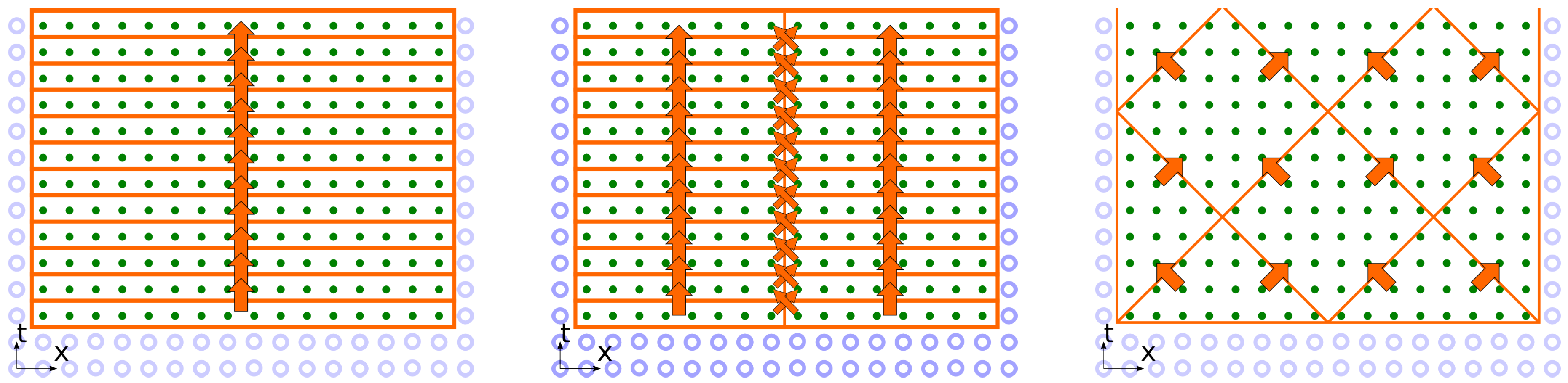
Let us give an example. The most prevalent way is to process the calculation one time iteration layer after another. The illustration (see Figure 4) by graph subdivision shapes is as follows: a $(d+1)$-dimensional box, which encompasses the whole graph of the problem, is subdivided into d-dimensional rectangles, containing all calculations on a certain graph layer. The order of computation in each such layer may be arbitrary: either a loop over all calculations, subdivision into domains for parallel processing or processing the cells by parallel threads.

Layer-by-layer stepwise calculation is used in almost all physics simulation software, and very few authors have ventured outside the comfort zone. The most notable unfavorable consequences are that during processing each time layer, the whole data array should be loaded from memory and stored into it, and the parallel processors have to be synchronized. There exist many other dependency graph traversal rules, which require much less synchronization steps and much less memory transfer. More operations may be carried out on the same data. One example is in Figure 4, which arises from tracing dependency/influence conoids.

We shall show now how the optimal algorithm is constructed for a given problem (the wave equation with cross-shaped stencil) and for a given implementation environment (GPGPU with CUDA). The illustration is given for a two-dimensional problem with $d=2$ in x-y axes. The dependency graph is plotted in 3D x-y-t space. If we treat each vertex as the processing not of one, but of $Nz$ elements, then this illustration is also applicable for 3D simulation problems. Such DiamondTile decomposition is assumed for all further discussions.

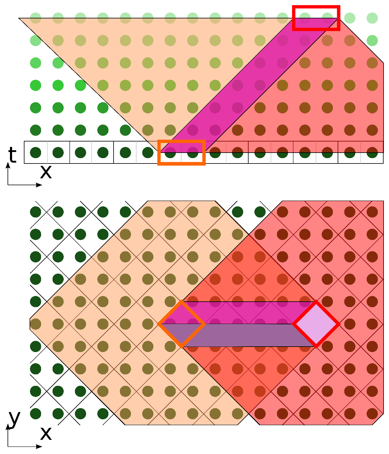
• The most compact shape that encompasses the stencil in space coordinates is a diamond. The 2D computational domain is subdivided into diamond-shaped tiles. For $N_O=2$, each tile contains two vertices.
• One diamond tile is chosen on the initial layer. Its influence conoid is plotted. After $Nt$ layers, we choose another tile, which lies near the edge of the influence conoid base, on the far side in the positive direction of the x-axis. Its dependence conoid is plotted.
• On the intersection of conoids, we find a prism (Figure 5).

This prism is a basic decomposition shape for DiamondTorre algorithms. Since it is built as an intersection of conoids, the subdivision retains correct data dependencies, and since the shape is a prism, all space may be tiled by this shape (boundary algorithms are the only special case).

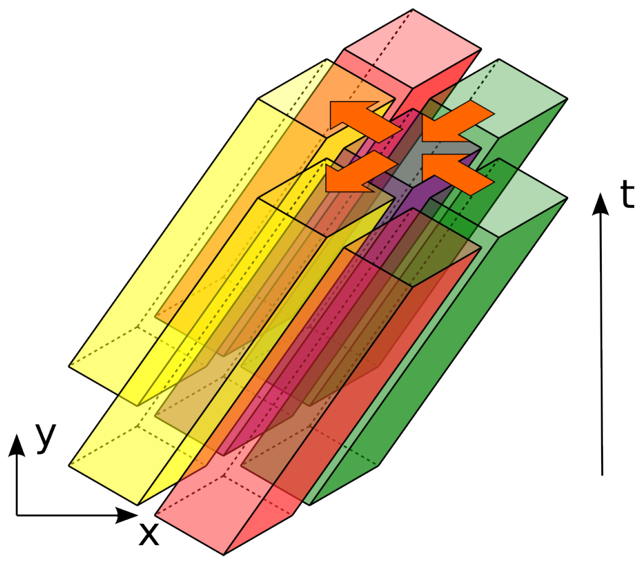
Each prism has dependency interconnections only with the prisms, the bases of which are directly adjacent to the base of this prism (see Figure 6). That is, the bases have common edges. The calculations inside the prism depend on the calculation result of the two right prisms and influence the calculations inside the two prisms to the left. The crucial feature is that the calculations inside the prisms with the common y coordinate, even those for which the bases touch each other, are absolutely independent.

A certain freedom remains with the calibration of prism parameters: height and base size. The distance from the stencil center to its furthest point is defined as a stencil half size and equals $ShS\equiv N_O/2$. By default, the base of the prism contains 2·$ShS$${}^2$ vertices. It may be increased in $DTS$ (diamond tile size) times along each axis, then the base would contain 2·$Sh{S}^{2}DT{S}^2$ vertices. The height of the prism equals $Nt$. $Nt$ should be divisible by two and $DTS$.

5. Benefits of the LRnLA Approach

The goal of the introduction of these algorithms is the solution of the issues that were presented in the Introduction, namely, the reduction of the requirements for memory bandwidth and the increase of asynchrony.

To quantitatively compare different algorithms of wave equation modeling in terms of memory bandwidth requirements, we introduce measures of the locality and asynchrony of an algorithm. The locality parameter is defined as the ratio of the number of dependency graph vertices inside the algorithm shape to the number of graph edges that cross the shape’s boundaries. The asynchrony parameter is equal to the number of vertices that may be processed concurrently.

The higher the parameters of locality and asynchrony are, the higher the performance that can be reached for memory-bound problems. While the locality parameter is generally not as high as it could be, the asynchrony parameter is often redundantly large. It is imperative not to increase the asynchrony parameter, but to correctly distribute the concurrent computation on different levels of parallelism.

The locality parameter has a similar meaning as the “operational intensity” measure introduced in the roof line model [25], but differs by a certain factor. The factor is defined from the scheme stencil and is equal to the number of operations per one cell per one time step divided by the data size.

Let us calculate the locality parameters for the algorithms that are introduced above as a subdivision of the dependency graph. For one dependency graph vertex, the locality parameter is equal to $1/(3+3N_O)$. This subdivision may be illustrated as enclosing each vertex in a box. We will call such an algorithm “naive”, since it corresponds to the direct application of the scheme (3) without accounting for caching ability specifics on contemporary computers with hierarchical memory subsystem organization.

A row of cell calculations along one axis is asynchronous on one time step. Fine-grained parallelism can be utilized by vectorizing the loop of $Nz$ elements along one (z) axis. The locality parameter increases to $1/(3+2N_O)$; the asynchrony parameter is $Nz$.

More generally, the locality parameter may be increased in two ways. The first method is to use the spatial locality of the data of a stepwise algorithm (Figure 4). The quantity of data transfers may be reduced by taking into account the overlapping of the scheme stencils. If a scheme stencil stretches in k layers in time ($k=3$ for the chosen scheme above), it is necessary to load data from $k-1$ layers and to save the data of one time layer. The locality parameter is equal to $1/k$, and this value corresponds to a maximal one for all stepwise algorithms. It is reached only if the algorithm shape covers all vertices of one time layer. In practice, this algorithm is impossible since there is not enough space on the upper layers of the memory subsystem hierarchy (which means the register memory for the GPGPU) to allocate the data of all of the cells in the simulation domain.

Taking the limited size of the upper layer of the memory hierarchy into account, we choose the tiling algorithm with a diamond shape tile as the optimal one. It corresponds to the DiamondTorre algorithm with $Nt=1$, so it is also a variation of a stepwise algorithm. Since the stencil occupies three time layers, two arrays are needed for the data store in the implementation, which are updated one-by-one in a similar fashion. The number of operations for one diamond update is equal to the number of vertices inside one diamond (2·$DT{S}^{2}Sh{S}^2$) times the number of operations for one vertex. To compute, we need to load 2·$DT{S}^{2}Sh{S}^2$ cells’ data to be updated (first array), 2·$(DTS$·${ShS+ShS)}^2$ cells’ data required for the update (second array) and save 2·$DT{S}^{2}Sh{S}^2$ updated cells’ data (first array). The locality parameter in this case is equal to $1/(3+2/DTS+1/DT{S}^2)$, and it differs from the optimal one ($1/k=1/3$) by a factor of two or less. The asynchrony parameter reaches $Nz$·$2DT{S}^{2}Sh{S}^2$ since all vertices in a horizontal DiamondTorre slice are asynchronous.

The further increase of the locality may be reached through temporal locality, namely by the repeated updating of the same cells, the data of which are already loaded from memory. The DiamondTorre algorithm contains $2Sh{S}^{2}DT{S}^2$ cell calculations on each of $Nt=2DTS$·n (n is some integer number) tiers and requires $2Sh{S}^2{(DTS+1)}^2-2Sh{S}^{2}DT{S}^2$ loads and $2Sh{S}^{2}DT{S}^2-2Sh{S}^2{(DTS-1)}^2$ saves on each layer, as well as $4Sh{S}^{2}DT{S}^2$ initial loads and $4Sh{S}^2{(DTS-1)}^2$ final saves. The locality parameter for one DiamondTorre amounts to:

$$DTS·n/(4n+2-2/DTS+1/DT{S}^2)$$

(4)

and approaches $DTS/4$ with large $Nt$.

At this step, the transition from fine-grained to coarse-grained parallelism takes place. For a row of asynchronous DiamondTorre (with a common y coordinate), the asynchrony parameter is increased by a factor of $Ny/(2DTS$·$ShS)$, which is the number of DiamondTorres in a row. The locality parameter increases to:

$$DTS·n/(n(4-1/DTS)+2-2/DTS+1/DT{S}^2)$$

(5)

and approaches $DTS/(4-1/DTS)$ with large $Nt$.

If the asynchrony of DiamondTorres with different x (and t) positions is involved, the coarser parallel granularity may be utilized. The asynchrony parameter would increase by about $Nx/(2Nt$·$ShS)$ times.

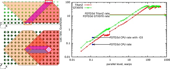
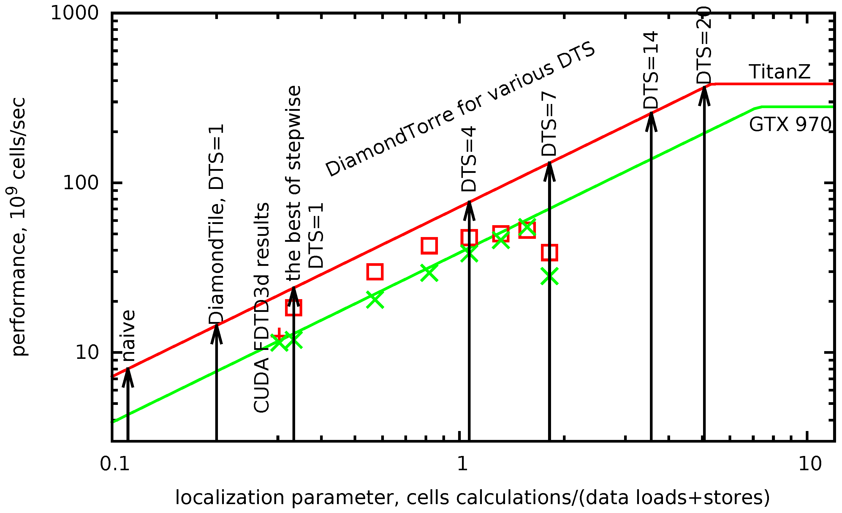
The roof line model may be plotted with the localization parameter as its horizontal axis. In Figure 7, roof lines for the two target GPUs are plotted in red and green lines. The maximum possible performance for a given algorithm is found as a ceiling point for its localization parameter (black arrows).

The major difference between the mentioned LRnLA algorithms and trapezoid tiling [14] is the predefined homogeneity of shapes. Trapezoid subdivision seeks for an optimal subdivision for an arbitrary space-time mesh. As a result of this optimization, shapes may differ. These optimized shapes include the ones similar to DiamondTorre in 1D, but others have lower locality. In the LRnLA method, both ConeFold and DiamondTorre shapes are taken as the optimal ones from the theoretical estimates of locality and asynchrony. Only a finite set of shape parameters is left for optimization. One advantage of this approach is the homogeneity of shapes, so the code is comparatively simple, and the overhead is minimized. The developed theory also provides performance estimates before the algorithm is implemented in code.

Anther approach for space-time subdivision uses a similar term diamond tile [15]. The diamond in that paper works differently, since the shape is in the space-time axis (x-t for 1D, like in Figure 4). DiamondTile in DiamondTorre spans the x-y axis. The idea in [15] works only for the 1D domain. For 2D and 3D, the evident generalization of this shape does not tile the whole simulation domain. When modeling in higher dimensions, it is necessary to provide additional shapes or to change the algorithm. The evident disadvantage of the former is the lower locality coefficient of some of these shapes.

The example of the latter is the wavefront diamond blocking method [16,17]. The advantage of DiamondTorre in comparison to these is an efficient use of the GPGPU architecture. The data on one DiamondTorre tier fit into the GPGPU register and may be processed asynchronously. This covers GPGPU device memory latency. The data used by DiamondTorre fit in the device memory, so the sliding window approach may be used to solve big data problems by utilizing whole host memory without the drop in performance [24].

6. CUDA Implementation

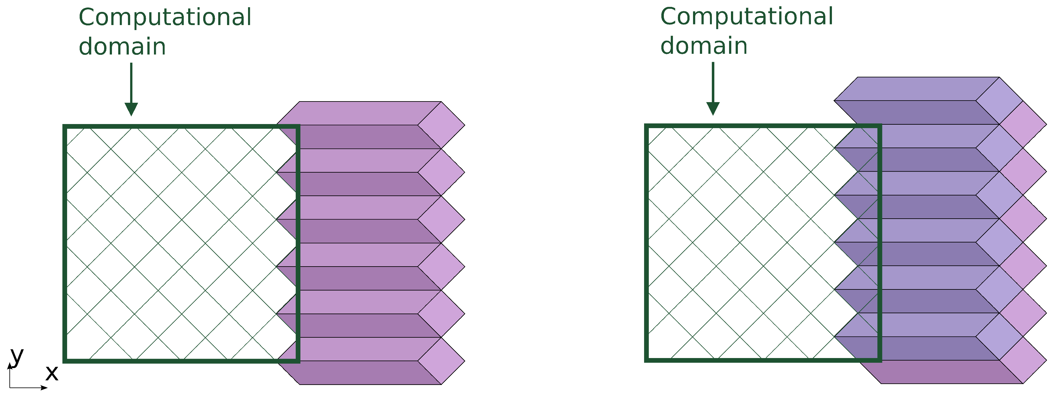
The computing progresses in subsequent stages. A stage consists of processing a row of DiamondTorre algorithm shapes along the y axis (Figure 8 and Figure 9). They may be processed asynchronously, since there are no dependencies between them on any time layers. They are processed by CUDA blocks. Each element of the 3D dependency graph that was subdivided into prisms corresponds to the processing of $Nz$ elements for 3D problems. Therefore, in each DiamondTorre $Nz$, CUDA threads process cells along the z axis. The DiamondTorre function contains a loop over $Nt$ time layers. Each loop iteration processes cells that fall into the DiamondTile.

It should be noted that as asynchronous CUDA blocks process cells in DiamondTorre in a row along the y axis, the data dependencies are correct even without synchronization between blocks after each time iteration step. The only necessary synchronization is after the whole stage is processed. However, since there is no conoid decomposition along the z axis, CUDA threads within a block should be synchronized. This is important to calculate finite approximations of the $\frac{{\partial }^{2}F}{\partial z^2}$ derivative. When the CUDA thread processes a cell value, it stores it in shared memory. After synchronization occurs, the values are used to compute the finite sum of cell values along the z axis. This way it is assured is that in one finite sum, all values correspond to the same time instant.

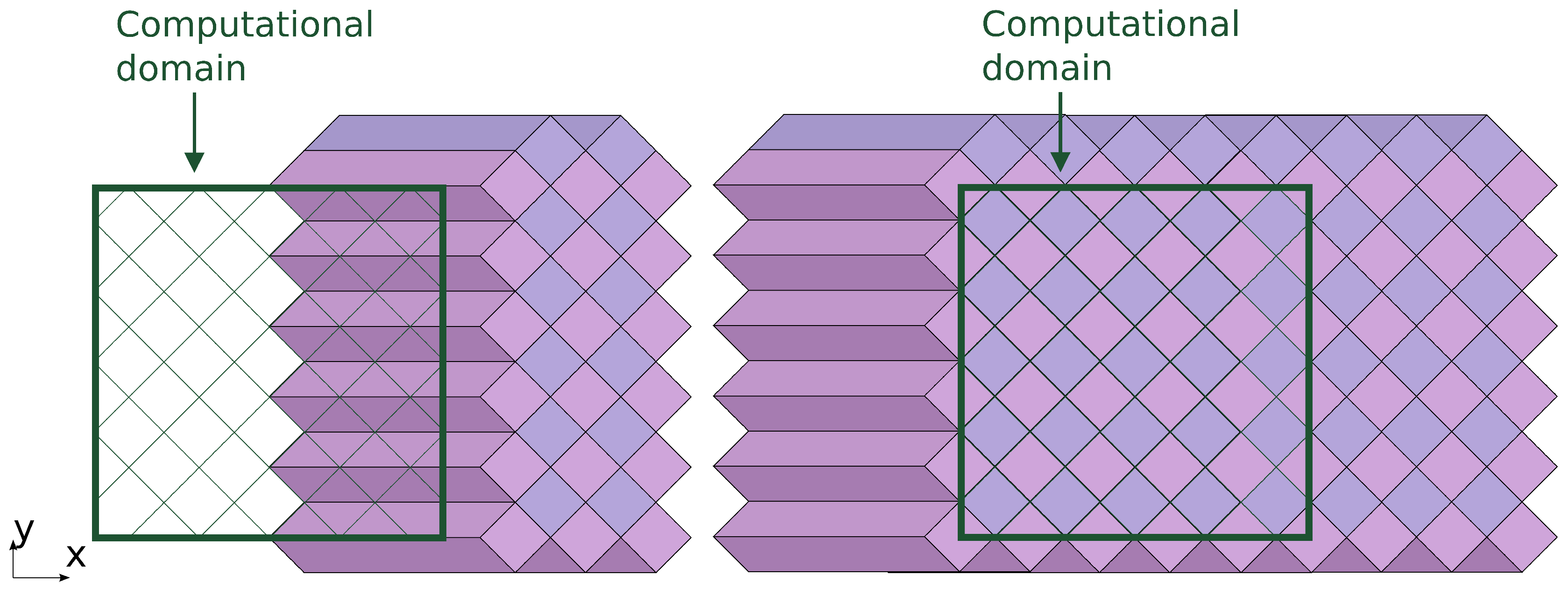
The next stage processes a row of DiamondTorre’s that is shifted by $ShS·DTS$ in the negative x direction and by the same amount in the positive y direction. The row is processed like the previous one, and the next one is shifted again in x and y, so that by alternating these stages, all of the computation domain is covered.

The first of these rows starts near the right boundary of the domain (Figure 8). The upper part of the prisms falls outside the computation domain. These correspond to the boundary functions, in which the loop over the tiles has fewer iterations, and the last iterations apply boundary conditions. After boundary prisms are processed (Figure 9), we arrive at the situation when in some cells of the computation domain, the acoustic field has the values of the $Nt$-th iteration step; in some cells, the field has its initial values; and other cells have values on time steps ranging from zero to $Nt$. After all stages are processed, all field values reach the $Nt$-th time step.

All calculations at each time are conducted in a region near the slope on the current DiamondTorre row. This property can be used to implement a so-called “calculation window”. Only the data that are covered at a certain stage have to be stored in the device memory; the rest remains in the host memory. This way, even big data problems can be processed by one GPGPU device. If the calculation time of one stage equals the time needed to store the processed data and load the data to be processed at the next stage, then the computation reaches maximum efficiency.

To enable multi-GPGPU computation, the calculation on each stage may be distributed by subdividing the DiamondTorre row in the y axis into several parts, equal to the GPGPU number [24]. The following illustrates a code sample ($N_O=2$, $DTS=4$), excluding complications at the boundaries. f and g correspond to the two arrays for subsequent time layers.

__shared__ float2 ExchZ[8][Nz];
#define SH_c(i) ExchZ[i][threadIdx.x]
struct Cell { float F[Nz], G[Nz]; };
__global__ void __launch_bounds__(Nz, 1+(Nz<=320)) //regs limit for Nz>320
weq_calcO2_DDe(int Ntime, int ixs0, int ixa0) {
 Cell* c0=...;//set pointer to tower’s bottom base cell
 register float2 f00={LS(F,-5,0),LS(F,-4,0)};//load data of tower’s bottom
 register float2 f10={LS(F,-4,1),LS(F,-3,1)};//from device memory
 register float2 g00={LS(G,-4,0),LS(G,-3,0)};//using macro LS and pointer c0,
 register float2 g10={LS(G,-3,1),LS(G,-2,1)};//then localize in 64 registers
 ...
 for(int it=0; it<Ntime; it+=8) {
   //DTS=4, 4 pair tiers per loop iteration, 4*4*4*2=128 cells steps
   SH_c(0) = make_float2(f00.y,f01.x);//put data to the shared memory for
   z-derivative
   SH_c(1) = make_float2(f10.y,f11.x);//float2 for Kepler’s optimization
   SH_c(2) = make_float2(f20.y,f21.x);
   SH_c(3) = make_float2(f01.y,f02.x);
   __syncthreads();//calculations chunk separation
   g00 = K1*make_float2(f00.y,f01.x) - g00 + K2*(SH_p(0)+SH_m(0)+f00+f01+f10+f31);
   //cross-stencil; SH_p, SH_m are the macros for getting iz+1, iz-1 data
   from shared memory
   LS(G,-4,0) = g00.x; LS(G,-3,0) = g00.y; //store recalculated
   (up to 8 times) data
   f00.x = LS(F,-1,4); f00.y = LS(F, 0,4); //load data from device memory
   g10 = K1*make_float2(f10.y,f11.x) - g10 + K2*(SH_p(1)+SH_m(1)+f10+f11+f20+f01);
   LS(G,-3,1) = g10.x; LS(G,-2,1) = g10.y; f10.x = LS(F, 0,5); f10.y = LS(F, 1,5);
   g20 = K1*make_float2(f20.y,f21.x) - g20 + K2*(SH_p(2)+SH_m(2)+f20+f21+f30+f11);
   LS(G,-2,c0,2) = g20.x; LS(G,-1,2) = g20.y; f20.x = LS(F, 1,6);
   f20.y = LS(F, 2,6);
   g01 = K1*make_float2(f01.y,f02.x) - g01 + K2*(SH_p(3)+SH_m(3)+f01+f02+f11+f32);
   SH_c(4) = make_float2(f31.y,f32.x);
   SH_c(5) = make_float2(f22.y,f23.x);
   SH_c(6) = make_float2(f13.y,f10.x);
   SH_c(7) = make_float2(f32.y,f33.x);
   __syncthreads();
   ...
   c0 += 2*Ny;//jump to next tower’s tier
 }
 ...//store data from top tower’s tier
}

This kernel is called in a loop. Each stage (row of asynchronous DiamondTorres) is shifted to the left from the previous one.

for(int ixs0=NS-Nt; ixs0>=0; ixs0--) {
   weq_calc_O2_DD<<<NA, Nz>>>(Nt, ixs0, 0); //even stage
   weq_calc_O2_DD<<<NA, Nz>>>(Nt, ixs0, 1); //odd stage
}
      

7. Results

The algorithm has been implemented for the finite difference scheme described in Section 3. In the initial values, we set a spherical wave source. The values on boundaries are set to zero and not updated.

The performance of the code is tested for various values of the $Nt$, $DTS$, $N_O$ parameters. The grid size was chosen as the maximal that fits the device memory (approximately 3.5 × ${10}^8$ cells and 1.5 × ${10}^8$ for 750Ti). Due to the algorithm shape, the code efficiency depends on its dimensions. The $Nx$, $Ny$, $Nz$ values that comprise this total cell number were varied, and the optimal result is taken for the graph. A few hundreds of time steps were taken to measure the efficiency.

In Figure 7, the achieved results for the second order of approximation are plotted under the roof line. The lowest point corresponds to the result of a sample code from the built-in CUDA examples library, “FDTD3d”. result from the built-in CUDA examples. It should be noted that the comparison is not exactly fair, since in FDTD3d, the scheme is of the first order in time and uses a stencil with one point less ($k=2$). Other points are from the computation results with the DiamondTorre algorithm with increasing $DTS$ parameter, $Nt=100$.

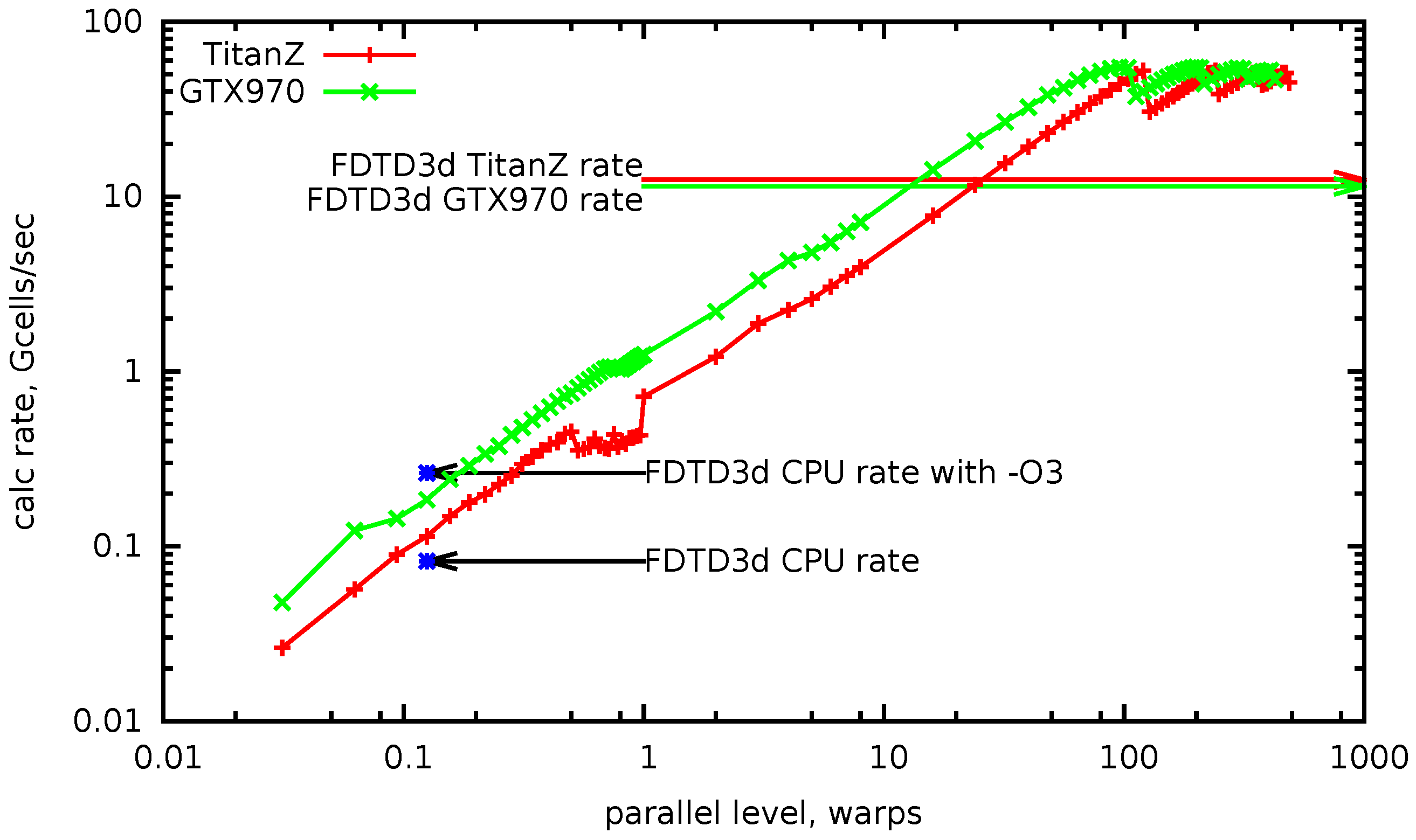
In Figure 10, the calculation rate is plotted versus parallel levels, measured in warps. It is measured as a strong scaling, for a calculation mesh of about ∼0.5 × ${10}^9$ cells. From $1/32$ to one on the horizontal axis, the number of used GPGPU threads rises from one to 32. This corresponds to the growth of $Nz$, while $Ny$ is minimal (one DTS), and $Nx$ is scaled to occupy all device memory. The increase in the calculation rate is satisfactorily linear. After one, the parallel levels increase by adding whole warps up to the maximum number of warps in the block (eight), with the number of enabled registers per thread equal to 256. As before, only $Nz$ grows, and $Nx$ is scaled down proportionally. After this, the number of blocks is increased, which corresponds to the $Ny$ growth. The increase of the calculation rate remains linear until the number of blocks becomes equal to the number of available multiprocessors. The maximum achieved value is over 50 billions cells per second.

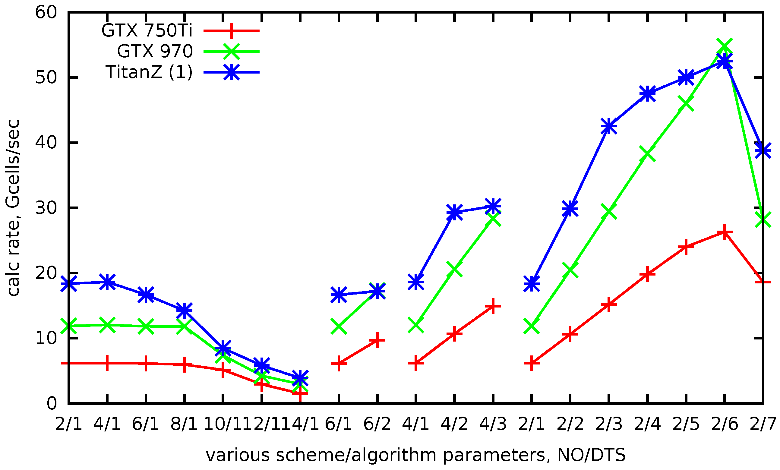
In Figure 11, the achieved calculation rate for different parameters is plotted. The labels on the horizontal axis are in the form $N_O/DTS$. Overall, the results correspond to the analytical predictions (5). With fixed $DTS=1$ and $N_O$ = 2, 4, 6, 8 (first four points), the calculation rate is constant (for Maxwell architectures), although the amount of calculation per cell increases. This is explained by the fact that the problem is memory bound. The computation rate increases with $DTS$ for constant $N_O$, since the locality parameter increases. For the rightmost points of the graph, the deviation from the analytical estimate for Kepler architecture is explained by insufficient parallel occupancy.

8. Generalization

The area of DiamondTorre application is not limited to acoustic wave equation. It has also been successfully implemented for finite difference time domain methods (FDTD) [26], the Runge–Kutta discrete Galerkin method [22,27] and particle-in-cell plasma simulation [23]. The LRnLA method of algorithm construction may also be applied for any other numerical methods with local dependencies and other computer systems and methods of parallelism.

9. Conclusions

The algorithm DiamondTorre is constructed to maximize the efficiency of stencil computations on a GPU. The theory to estimate its performance is developed, based on the roof line model and two algorithm parameters: locality and asynchrony. The algorithm is implemented in code, and the performance has been tested for various algorithm parameters. The result show the expected increase of performance in comparison with stepwise methods and agrees with the quantitative estimates. The goal to efficiently utilize all parallel levels of the GPU device and all if its memory is achieved. For the scheme with the second order of approximation, the calculation performance of 50 billion cells per second is achieved, which exceeds the result of the best stepwise algorithm by a factor of five.