1. Introduction
Computational simulation of complex phenomena can provide answers to problems for which no experimental data or theoretical studies are available, but it requires robust, efficient, and accurate numerical models. The problem considered in this paper is of evolution of methane hydrate, which is an ice-like substance present in large amounts in subsea sediments, and which plays an important role both as a potential energy source and environmental hazard as well as in global climate studies [
1,
2].
In the paper [
3] we introduced a reduced model for methane hydrate formation in variable salinity conditions and provided details on the equilibrium phase behavior adapted to a case study from Ulleung Basin. One of the advantages of this reduced model in contrast to fully comprehensive models such as in, e.g., [
4], is that the reduced model is easy to implement and to extend, and is amenable to various analyses.
In this paper we describe the computational aspects of the model, with the emphasis placed on the variants of time-stepping. Our reduced model accounts for three components: water, methane, and salt, and two phases: aqueous, and solid (hydrate). Thus, it places in the general framework of multiphase multicomponent models such as those in [
5,
6,
7] for which accuracy and efficiency have been studied extensively in the past decades. In particular, for the oil-water or black-oil models described e.g., in [
8,
9,
10,
11,
12,
13] the best practice is to use mass-conservative spatial schemes combined either with an implicit treatment of pressures and explicit treatment of saturations/concentrations, or with a fully implicit treatment of all phases and components. Typically, the computational complexity of implicit models is the highest, while other variants are easier to implement. In compositional models [
14] with
M components the pressure solver is complemented with
M−1 transport equations solved for concentration of the selected
M−1 species, and followed by flash,
i.e., the equilibrium solver. The typical time scales of interest for reservoir simulation with these models are days to decades of production or environmental remediation. On the other hand, in [
3] and here we are interested in long-term behavior and hydrate basin modeling, and it makes sense to assume that the pressures and temperatures are known and given by hydrostatic and geothermal distributions. Our models need only to resolve the interdependence between methane and water phase equilibria that depend on the presence of salt, and our time-stepping algorithms have different features than those for the oil-gas reservoir simulators.
We implement the interdependence between the components and phases as follows. The water-methane-salt equilibria are handled using the approach of nonlinear complementarity constraints, and are either tightly or loosely coupled to the salt mass conservation; their implementation is especially easy with the reduced phase behavior model adopted in [
3]. We consider and compare three variants of time-stepping that realize these tight or loose couplings: the fully implicit (I), semi-implicit (SI), and sequential (SEQ) algorithms. The comparison that we carry out is intended to demonstrate the merits of these approaches, and guide the choice of a model.
In addition, in this paper we test the sensitivity of the approach to the assumed phase behavior model, as well as to various parameters defining the discretization. The latter is new and was not undertaken for the comprehensive model [
4]. It is significant in that it guides the reader in the choice of optimal parameters and shows the robustness of the reduced model.
The paper is organized as follows. In
Section 2 we briefly recall the model proposed in [
3] including the phase behavior. In
Section 3 we describe in detail the time-stepping variants and spatial discretization for that model. In
Section 4 we compare the I, SI, and SEQ time-stepping variants, and in
Section 5 we discuss the sensitivity of the model to the various parameters of the computational model. We conclude in
Section 6.
2. Mathematical Model
In the last decade two classes of models for hydrates have been used to describe hydrate behavior in natural systems. These are the fully comprehensive equilibrium models such as [
4], and the simpler conceptual models [
2,
15,
16], in which simplified mechanisms for fluid equilibria and/or kinetics were assumed. The model presented in [
3] and discussed here falls somewhere inbetween, and is a direct simplification of the comprehensive model in [
4]. The simplicity of the reduced model allows for rigorous mathematical well-posedness analysis in the case of the diffusive transport in [
17], and more general analysis in [
18] for advective/diffusive transport.
We consider the transport of methane and salt in the sediment reservoir
. The notation used throughout is provided in
Table 1. Each point
is at some depth
below the sea surface, with the origin
at the bottom of the Gas Hydrate Stability Zone (GHSZ). At the seafloor,
i.e., at the top of the reservoir Ω, we have
where
L is the thickness of the hydrate zone. Next, at the seafloor, the depth of water above seafloor is the reference depth
, so the sea surface is at
. We also set the coordinate
measured in mbsf (meters below seafloor) which is used in other models [
19]. In the general case of a 2D or 3D reservoir the bathymetry is variable, thus
is measured relative to the (constant) sea surface rather than to the seafloor.
Table 1.
Notation and definitions (kg/kg, per kg of liquid phase).
Table 1.
Notation and definitions (kg/kg, per kg of liquid phase).
| Symbol | Definition | Units/value |
|---|
| Data about reservoir and fluids |
| Spatial coordinate | [m] |
| t | Time variable | [yr] |
| G | Gravitational acceleration | 9.8 |
| Depth of point x from sea level | [m] |
| Seafloor depth | [m] |
| | In 1D case , | |
| Depth below seafloor | [m] |
| (G)HSZ | (Gas) Hydrate stability zone | |
| P | Pressure | [Pa,MPa] |
| Hydrostatic gradient | |
| T | Temperature | [K] |
| Geothermal gradient | [K/m] |
| q | Darcy volumetric flux of liquid phase | [m/yr] |
| Diffusivity of component C in the liquid phase | [/yr] |
| | | |
| Seawater density | 1030 |
| Hydrate density | 925 |
| Mass fraction of methane in hydrate phase | 0.134 kg/kg |
| Constant used for methane concentration | 0.1203 kg/kg |
| Porosity in Ω without/with hydrate present | |
| Permeability in Ω without/with hydrate present | |
| Seawater salinity | 0.035 [kg/kg] |
| Supply of methane (source/sink term) | [kg/kg/yr] |
| α | Parameter of the reduced model | [kg/kg] |
| Variables in the model |
| Void fraction of liquid and hydrate phases | |
| Mass fraction of methane (solubility) in liquid phase | [kg/kg] |
| Mass fraction of salt (salinity) in liquid phase | [kg/kg] |
| Mass concentration of methane and salt | [kg/kg] |
In this paper as in [
3] we assume that the conditions in Ω are favorable for hydrate presence and that Ω is entirely within the GHSZ, while the methane is supplied by advection and diffusion from beneath GHSZ. We also assume that
is known and follows the geothermal gradient
where
is the temperature at some reference depth
and
is the geothermal gradient; see [
3] for experimental values. The pressure
is assumed close to the hydrostatic
Here is known at the reference depth .
Finally, the actual porosity available to the liquid phase at x is , where is the liquid phase saturation, i.e., void fraction of the liquid phase. The actual permeability in the presence of hydrate is an important property. However, it is not needed in the 1D model with a constant flux and an assumed hydrostatic pressure distribution.
2.1. Mass Conservation
In region Ω we have the following mass conservation equations for methane and salt components, respectively
with the definitions
where
R is given in
Table 1. The model is complemented by a pressure equation or
q must be given; here we assume the latter. As we explain in [
3], the Equation (
3) arises as a special case of the first-principles comprehensive model in [
4].
We see that in Equation (
3) we have two mass conservation Equations (3a,b) with three unknowns that must be chosen from
and
. To close the system we use the nonlinear complementarity constraint abbbreviated below as [NCC-M] phase constraint. We explain it below.
2.2. Phase Equilibria and [NCC-M] Constraint
The (maximum) amount
of methane that can be dissolved in the liquid phase depends on the pressure
P, temperature
T, and the salinity
. Equivalently, these variables determine the circumstances in which
and
,
i.e., when the hydrate phase can be present. In addition,
determines how the total amount of methane
is partitioned between the liquid and hydrate phases. This phase equilibrium is expressed concisely as a nonlinear complementarity constraint [NCC-M]
In other words, if is small enough so that , then only the liquid phase is present , and is the independent variable that describes how much methane is dissolved in the liquid. On the other hand, when the amount present , the excess amount of methane above forms the hydrate phase with , and becomes the independent variable while . This relationship has to be satisfied at every point .
2.2.1. Data for
In the hydrate literature [
4,
20] there are tabulated data, or algebraic models, for how
depends on
. In addition, there may be dependence of Equation (
3e) on the type of sediment [
19,
21] but this is out of scope here. In [
3] we developed a particular approximation
in which the data
and
must be provided. This approximation Equation (
4) includes as a special case the algebraic model in [
19]. In [
3] we describe how to obtain
and
by a fit to the lookup tables extracted from the well known phase equilibrium software CSMGem [
22], and we calibrate them for the typical depth, temperature, and salinity conditions found in Ulleung Basin; see [
3] and
Section 5. As is well known,
increases with depth, thus decreases with
x. On the other hand,
found with CSMGem is positive while the authors in [
23] believe it should be negative; see [
3] for details. In
Section 5 we discuss the sensitivity of the model to the assumed profile of
.
2.2.2. Other Constraints
There are additional constraints that are not part of Equation (
3) but are motivated by the physical meaning of the variables
, and
. In particular, we must have
or
With some assumptions on
, the boundary and initial data, and small
one can prove that Equation (
5) holds as a consequence of the maximum principle and other abstract analyses. (See [
17] for the diffusive case and [
18] for advective and diffusive transport case).
In more general circumstances one cannot prove that Equation (
5) holds. In fact, a numerical model may readily produce
increasing to 1 and beyond. This clearly is nonphysical, since even before the pores become plugged up and
, all the flow and diffusion ceases, local pressures increase, and the sediment may break.
When Equation (
5) is violated, a model more general than Equation (
3) should be considered. In particular, such a model should include geomechanics and pore-scale effects; see, e.g., the conceptual model described in [
21]. However, the analysis of such a model is presently out of scope. In the model discussed in this paper we terminate the simulation when Equation (
5) does not hold.
2.3. Boundary and Initial Conditions
The model Equation (
3) must be supplemented with appropriate initial conditions imposed on
and
, and the boundary conditions on the fluxes or on the values of the transport variables
and
. In this paper we set
The conditions Equation (
6c) assign the seawater salinity at
and some other salinity
at HSZ known from observations. The conditions Equation (
6b) assume some methane present at HSZ
, and that there is no methane in the ocean at
. The choice consistent with Equation (
4)
allows the maximum possible amount of methane to be transported by advection and diffusion from underneath the HSZ.
3. Numerical Model
Now we provide details of the numerical model for Equation (
3). We use mass-conservative spatial discretization based on cell-centered finite differences (FD) with harmonic averaging and a nonuniform structured spatial grid. An alternative discretization of the case
, with Finite Elements and mass lumping, was considered in [
17], but it would not accommodate large advective fluxes and is not locally mass conservative. For time discretization we use operator splitting: we treat advection explicitly and diffusion implicitly as in [
24,
25,
26]. The diffusion/equilibria handle two components and are organized in several time-stepping variants. In each variant we have to solve a linear or nonlinear system of equations; for the latter we use Newton (or semismooth Newton) iteration.
After the discretization of Equation (
3), at each time step, one solves for the approximate values of the five unknowns
. (At this point we are not yet providing any notation specific to time steps or grid points). Note that Equation (
3c) and Equation (
3d) are merely the definitions of the terms used in the transport equations Equation (
3a), Equation (
3b) complemented by the phase equilibria Equation (
3e). Thus we can eliminate and actually solve only for three variables
the system of three equations which we write as
The details on discrete form of
and
which correspond to Equations (3a,b,e), respectively, are developed below. We discuss first the most difficult part of implementing Equation (
3e), then we provide details of discretization of the transport equations. The system Equation (
8) is nonlinear, and we discuss next the particular variants of the solvers and time-stepping variants.
3.1. Implementing Phase Constraint [NCC-M] in Fully Implicit Models
While it is well known how to discretize and solve advection-diffusion equations, implementing phase equilibria constraint Equation (
3e) is challenging. There are practical approaches which have been successfully implemented [
4,
7]. In addition, approaches known from constrained optimization [
27,
28] have been recently applied; see [
17,
29].
In the first class of approaches, the constraint Equation (
3e) can be rewritten using the notion of
active/inactive sets [
27]. In this approach at each time step and/or iteration, the (grid) points are identified as either those for which the first part of the inequality Equation (
3e) holds, or those where the other complementary inequality must hold. Next, the mass conservation equations are specialized depending on the state of the primary unknowns, and are grouped together and solved for the particular active set of independent unknowns. In summary, in each time step and/or iteration of the nonlinear numerical solver, the solver changes the vector of unknowns depending on which variables need to be used. In consequence, not just the values, but also the sparsity structure of the Jacobian matrix change from iteration to iteration. This approach is known as
variable switching [
4,
7] where at each gridpoint one identifies the appropriate independent variable depending on which of the inequalities holds.
In another equivalent approach one takes advantage of the semismooth “min” function as proposed in [
29]. We recall that the function “min(u,v)” equals
u if
and
v otherwise. We represent Equation (
3e) in an equivalent way as
In [
17] we showed that the “min” representation of Equation (
3e) is equivalent to variable switching discussed above. With the “min” function approach, Equation (
9) is a nonlinear equation in the variables
and
, and it provides the fifth equation to complement Equations (
3a)–(
3d) that can be solved together for the five unknowns
.
Since the function “min(u,v)” is piecewise linear and non-differentiable along
, it is also
semismooth [
28]. The theory of semismooth maps developed in [
28] allows us then to analyze the solvability of the resulting nonlinear system of equations.
We found that the approach using Equation (
9) is easy to implement and vectorize, and is modular,
i.e., it does not require that we rewrite the complex logic of active/inactive sets whenever there is need to expand the logic or the physics in the model. The potential disadvantage of using Equation (
9) is that the number of unknowns involved grows from two per grid point to three per grid point. In practice, however, this has minimal implications on the storage, since all the variables must be stored anyway. On the other hand, the size of the linear system that arises at each iteration when solving Equation (
8) is by 50% larger than the size of that with explicit variable switching. However, the matrices in the linear systems corresponding to both approaches are sparse. An efficient implementation of the “min” approach in which sparsity is fixed, can outweigh the cost of the variable switching approach in which the pattern of sparsity varies from iteration to iteration.
3.2. Implementing Phase Constraints in Non-Implicit Models
Some of the time-stepping variants other than fully implicit require local nonlinear solvers called “flash”. These are invoked at each grid point ans solve a system simpler than Equation (
3e) in which the values of one or of more of the variables are assumed known.
Simple flash. The simplest situation is when
is known and we know
. To determine
and
we simply use Equations (
3e), (
3c) to calculate
Simple flash only is applicable if salinity is fixed because of the dependence of on .
Two-variable flash. Given
we can solve for the three unknowns
,
,
using Equations (
3c), (
3d) and (
9). The implementation is especially easy if Equation (
4) is used. This flash solver typically takes 2 or 3 iterations to complete, but may fail when
is close to 1.
3.3. Notation in Fully Discrete Model
The notation for discretization is straightforward. We find approximations to the relevant variables at discrete time steps
The transport model Equation (
3) advances the model variables from
to
, with the time step
considered uniform for simplicity. Also for simplicity, we consider the 1D reservoir
, where
are the cells with the centers
and uniform length
h, and
. We approximate
and set
to be a vector of
, with analogous notation applied to other variables.
We start by integrating each of the mass conservation equations over each . We show the calculations for methane; the ones for salt are analogous.
Accumulation and source terms. For each
we calculate the approximation of accumulation and source terms as follows
Advection terms. It suffices to consider only methane advection, since salt advection si treated the same way. We consider first the case
. The advective flux
is handled by upwinding. Close to the inflow boundary at
, we set
to the boundary value
. If
, we replace the right hand side by
, and use the boundary condition
on top of the reservoir.
Diffusion terms. For the spatially dependent diffusion coefficient
and the variable
we have, in a standard way [
30,
31]
where
are found by harmonic averaging of the values
and
, respectively. Close to the boundary we apply the discretization described in [
32], e.g., at
in place of
we use the boundary value
, with
set to
.
We also define the discrete diffusion matrix
A with the entries defined so that
is equal to the right hand side of Equation (
13). In particular,
. With Dirichlet boundary conditions
A is symmetric and positive definite, as long as
. In 1d
A is also tridiagonal. Further, since
depends on
as in
Table 1, the matrix
depends on the local saturation values. Finally, since
and the type of boundary conditions on
matches that for
, the matrix for salt equation is the same as that for methane.
3.4. Advection Step
The time-stepping variants considered in this paper are explicit in the advection. This allows development of higher-order schemes as well as avoids additional numerical diffusion associated with implicit treatment of advection [
24,
25,
26]. With this step, we have to consider appropriate boundary conditions which in the operator splitting come from Equations (6b,c); in the advection step we can only impose the boundary condition on the inflow boundary.
In the 1D case considered here implies that q is constant, thus the inflow boundary is determined by the sign of q. If , the inflow bundary is at the bottom of the reservoir at , otherwise it is at . In the advection step, we must know and on the inflow boundary, and we use here exactly two of Equations (6b,c).
The advection step is as follows. Given
from previous time step, with the corresponding
, we can easily calculate
where the terms
are approximated by Equation (
12). Rearranging Equation (
14a) we obtain an explicit expression for the methane amount
at the intermediate auxiliary time
As is well known, stability of this explicit advection scheme requires that
via the well-known Courant-Friedrichs-Lévy (CFL) condition [
33] adapted to porous media.
Advection scheme for
is defined analogously to Equation (
15).
3.5. Diffusion Step
Knowing and from the advection step, we solve the coupled diffusion/phase behavior system for and with the boundary conditions Equations (6b,c). To distinguish between the variants and avoid additional superscripts, we reserve the notation and for the solutions to the fully implicit variant I.
First we recall that with Equation (
13) and matrix
A we have the vector equation
Note the time lagging of the dependence of matrix A on .
For
we have an equation analogous to Equation (
17). Additionally, we need to account for [NCC-M]. This coupled system of two component diffusion and phase equilibria is solved with one of the three variants: fully implicit (I), semi-implicit (SI), and sequential (SEQ). See
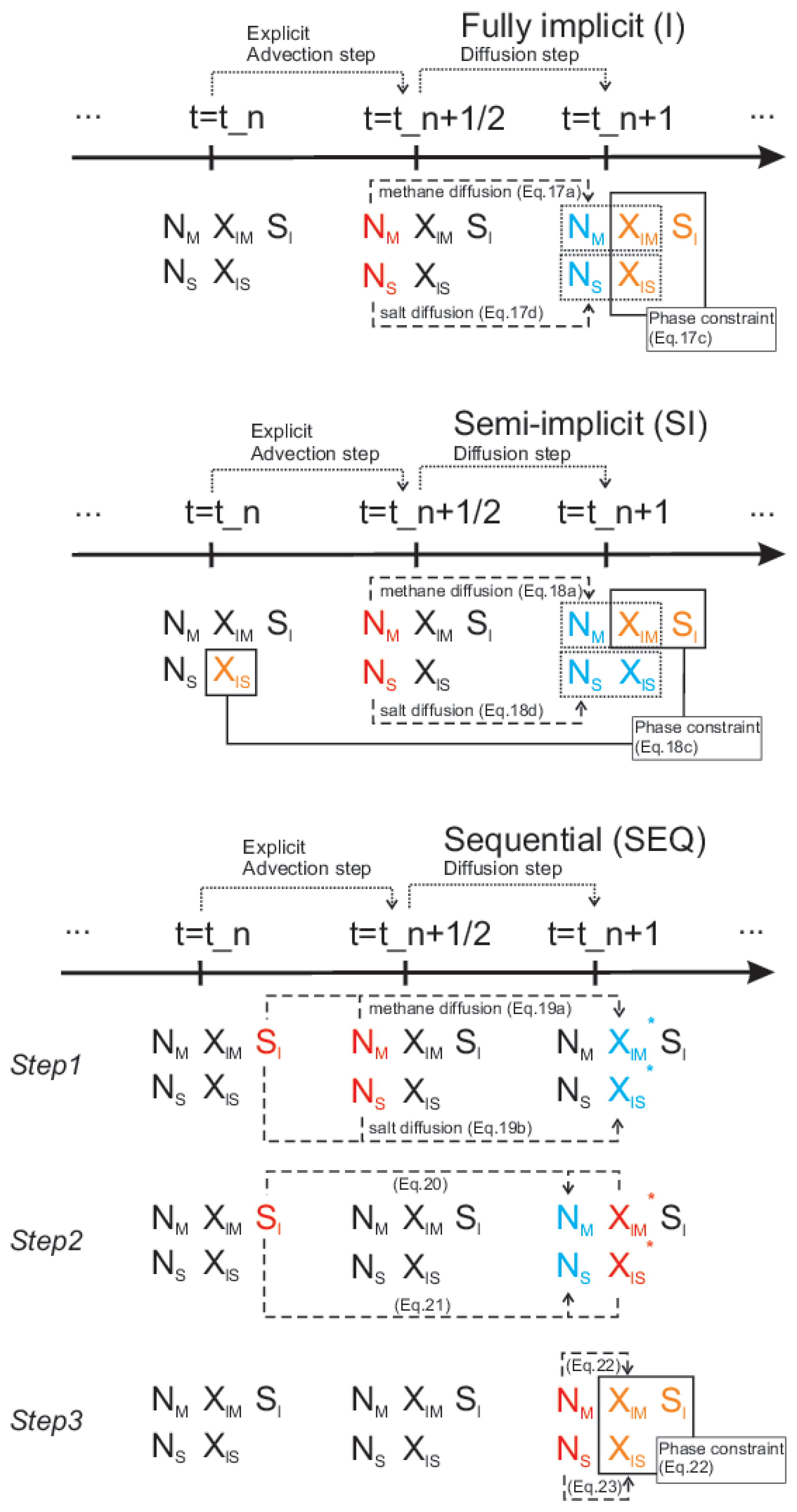
Figure 1 for graphical illustration of the operator splitting and different variants.
Figure 1.
Illustration of time stepping variants.
Figure 1.
Illustration of time stepping variants.
3.5.1. Variant (I): Fully Implicit
The fully implicit variant solves the coupled two-component diffusion/phase behavior system for
as follows
Here Equation (
18b) provides the definition of
needed in Equation (
18a), and is directly implemented in the code. The two unknowns in Equation (
18a) are
and
; these are connected to each other via Equations (
9) and (
4)
with the dependence on
defined directly by
The Equation (
18) is solved using Newton’s method for
, and the Jacobian of the system is a
sparse block matrix. Its form and particular pattern of sparsity depend on Equation (
18c). Note that in Equation (
18) we maintain full consistency of mass conservation between the time steps (up to the tolerance of nonlinear solver), as well as consistency of thermodynamic constraints.
3.5.2. Variant (SI): Semi-Implicit
The semi-implicit variant differs from Equation (
18) in the treatment of
in Equation (
18c). We time-lag
and remove the two-way coupling between the methane transport and salinity transport. Methane transport in this model is governed by
so that these equations are solved for
using Newton’s method. The Jacobian of the system is a
sparse block matrix.
Knowing
we can solve the system for
which is linear
while the mass conservation between the time steps is enforced in this variant, there is potential inconsistency in thermodynamic constraints introduced by the time-lagging in Equation (
19c). To correct this, we follow up with the two-variable local flash solver which corrects the saturations and solubilities while keeping
, and
fixed.
3.5.3. Variant (SEQ): Sequential
The sequential variant is the simplest to implement and one can easily adapt an existing advection-diffusion code. The advantage of this variant is that each of the global algebraic systems is linear. The disdvantage is that the phase behavior is not fully coupled to the transport dynamics, and fine time-stepping may be needed to ensure accuracy.
The SEQ variant time-lags the saturation variable in the methane and salinity transport equations
Note that the phase constraint is not imposed in Equation (
20), and that the equations are not coupled. We solve them for the temporary unknowns
, and next we recalculate the mass concentrations corresponding to the new solubilities from Equations (19b,e)
To keep these consistent with Equation (
9), we invoke the nonlinear two variable flash solver. Its input are the mass concentrations
, and its output are the final new values of solubilities
, and saturations
which satisfy the discrete version of Equation (
9) plus the mass concentration definitions
The flash solver for Equations 23–25 provides the consistency between the mass-related variables and thermodynamic constraints. However, the mass conservation between time steps is not strictly enforced due to time-lagging.
4. Comparison of Performance of the Time Stepping Variants
In this section we evaluate the accuracy, robustness and computational complexity of the proposed I, SI, and SEQ variants of hydrate models using realistic scenarios of methane hydrate formation in typical sediments. We also give details on what time steps appear reasonable, and how to choose discretization parameters.
In oil-gas reservoir simulation the fully implicit algorithms implement directly the backward Euler formula. The fully implicit formulations are usually the most accurate, but also most complex to implement. In turn, sequential and semi-implicit variants are typically less accurate but, at least in principle, they have smaller computational complexity per time step, and are easier to implement than the fully implicit algorithms. Typically, the results of non-implicit schemes converge to those of fully implicit models as . In fact, non-implicit variants may require small τ in in order to resolve, e.g., complicated phase equilibria, heterogeneity, or complex well behavior; the use of small τ somewhat erases the benefits of small computational cost per time step. The non-implicit variants may still have advantages in the easiness of implementation.
The computational experiments we set up to test the variants I, SI, and SEQ are built from the following base case similar to those in [
3] for the methane hydrate and salinity conditions in Ulleung Basin.
We set
with
m, and use uniform porosity
. We vary
q from large
m/yr for which advection dominates, to the case where diffusion is dominant and
m/yr. We assume that advection and diffusion provide the only transport mechanisms and that
, that is, the only sources of methane are from upward fluxes. For thermodynamics we use the reduced model Equation (
4) and [NCC-M] constraint is implemented with Equation (
9). Unless otherwise specified, we use the data
and
calibrated for Ulleung Basin and shown in [
3] and
Section 5 with the same boundary and initial conditions. We use zero initial conidtions for methane, and assume that the initial distribution of salinities varies linearly between the boundary conditions
and
. We run simulations until
, or until
reaches the unphysical values close to 1.
Discretization parameters are chosen as follows. We use
with
in the base case. The time step is subject to the CFL constraint Equation (
16). In particular for
the largest time step
yr.
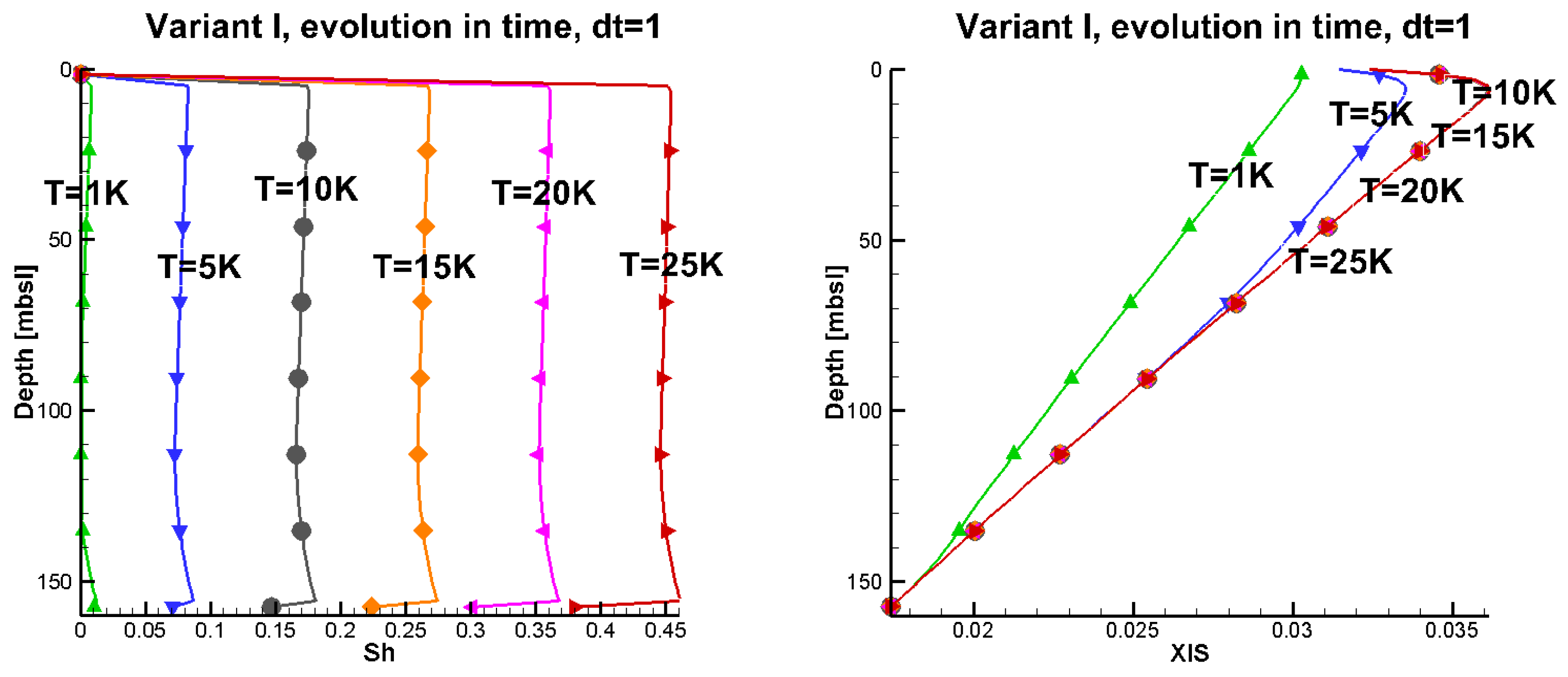
For illustration of the base case in
Figure 2 we show the evolution of
and
for the case
m/yr, with small
yr. In this case of strong advective flux the hydrate forms quickly and fills up the domain. These results are similar to those in [
3] and more generally to the test cases in [
4]. The evolution of salinity shows that there is a boundary layer close to the outflow which forms around
and remains unchanged afterwards.
Figure 2.
Evolution of hydrate saturation and of salinity for the base case. (left) Plot of , (right) Plot of . Variable equals at these times and is not shown.
Figure 2.
Evolution of hydrate saturation and of salinity for the base case. (left) Plot of , (right) Plot of . Variable equals at these times and is not shown.
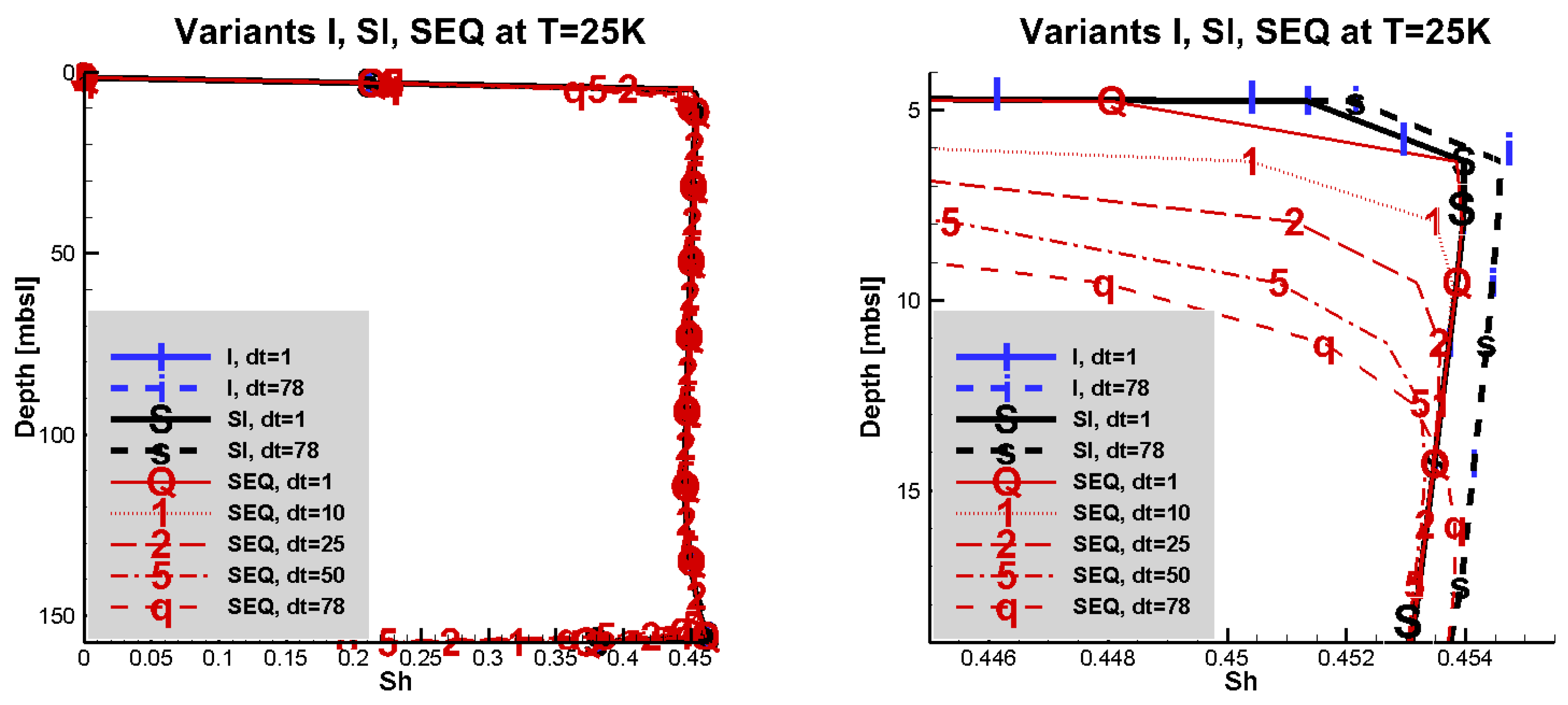
4.1. Accuracy of the Time-Stepping Variants and Choice of Time Step
Here we study the sensitivity to
τ which can guide its choice. In general, one wants to use small enough
τ obeying the upper bound (
16) and such that its further decrease does not have much influence. However, small
τ means large number
of time steps; this is significant in hydrate basin simulations since
may be easily
or more. Further, as suggested by our experience from oil-gas reservoir simulations [
10,
11,
13], we expect that for small
τ the results of the three variants I, SI, SEQ are very similar, and that for large
τ they differ.
In
Figure 3 we present the plots of
obtained for different
τ. Quantitative information supporting these observations is included in
Table 2. (We do not present details concerning the evolution of
since the results differ by less than 0.01% in each case.) We notice that the results corresponding to
and the variants I, SI, and SEQ are essentially indistinguishable; this degree of closeness is more than expected. In addition, the results corresponding to the largest advection step
and to the variants I, SI and SEQ are close to each other as well; they tend to overpredict those for
.
Figure 3.
Plots of for different time steps τ (denoted on figure by ), and different time-stepping variants fully implicit (I), semi-implicit (SI), and sequential (SEQ). (left) Plots over the full range of depth and are essentially indistinguishable. (right) The zoom of the left plot shows a small sensitivity to the choice of time step and of the model variant.
Table 2.
Maximum hydrate saturation obtained with different model variants and time steps at and , all parameters as in base case.
Table 2.
Maximum hydrate saturation obtained with different model variants and time steps at and , all parameters as in base case.
| τ | SEQ | SI | I |
|---|
| | |
| 78 | 0.177208 | 0.182844 | 0.182844 |
| 70 | 0.176441 | 0.181803 | 0.181803 |
| 50 | 0.176834 | 0.181267 | 0.181267 |
| 25 | 0.177841 | 0.180908 | 0.180908 |
| 10 | 0.178834 | 0.180736 | 0.180736 |
| 5 | 0.179238 | 0.180688 | 0.180688 |
| 1 | 0.180183 | 0.180651 | 0.180651 |
| | |
| 78 | 0.456162 | 0.463925 | 0.463925 |
| 70 | 0.456803 | 0.464271 | 0.464271 |
| 50 | 0.45644 | 0.462797 | 0.462797 |
| 25 | 0.457708 | 0.462438 | 0.462438 |
| 10 | 0.458886 | 0.462266 | 0.462266 |
| 5 | 0.459731 | 0.462218 | 0.462218 |
| 1 | 0.460878 | 0.462181 | 0.462181 |
In addition, we see that the model SEQ is potentially the most sensitive of all three to τ close to the boundaries and in areas with larger methane gradients. (This suggests the need for adaptive gridding). In addition, as τ decreases, the results tend to converge to the value for . Further decrease of τ (not shown here) does not influence the solution much, thus appears as the smallest sensible choice for this .
4.2. Robustness and Efficiency of the Variants
Above we established that the simulated hydrate saturation values do not seem to significantly depend on the time step τ or on the variant of time stepping. Next we consider the robustness of the variants and in particular, how they handle difficult physical circumstances such as when is large due to large advective fluxes.
In
Table 3 we report on the performance of the nonlinear solver, tested intentionally without any fine-tuning such as line-search. We see that between
and
all variants I, SI, SEQ struggle when
. The model I appears somewhat more robust than the other two and it can simulate the hydrate evolution up to higher values.
Table 3.
Robustness of nonlinear solvers depending on the variant and the time step for the simulations of the base case between and . The robustness is assessed by checking which solver variant is more prone or more robust to failing in the difficult modeling circumstances close to unphysical. We report the critical value obtained before the solver fails, and on the number of iterations. When is denoted by “-”, this means the solver did not complete. For SEQ model, denotes the number of flash iterations. For the SI and I models, denotes the number of global Newton iterations.
| τ | SEQ | SI | I |
|---|
| | | | | | | |
| 78 | 0.75833 | - | 0.767473 | - | 0.773341 | - |
| 70 | 0.772449 | - | 0.782752 | - | 0.781435 | - |
| 50 | 0.806955 | - | 0.817198 | - | 0.817198 | - |
| 25 | 0.873396 | - | 0.880766 | - | 0.880766 | - |
| 10 | 0.925712 | 2 | 0.932267 | 2 | 0.932267 | 3 |
| 5 | 0.926744 | 2 | 0.93222 | 2 | 0.93222 | 3 |
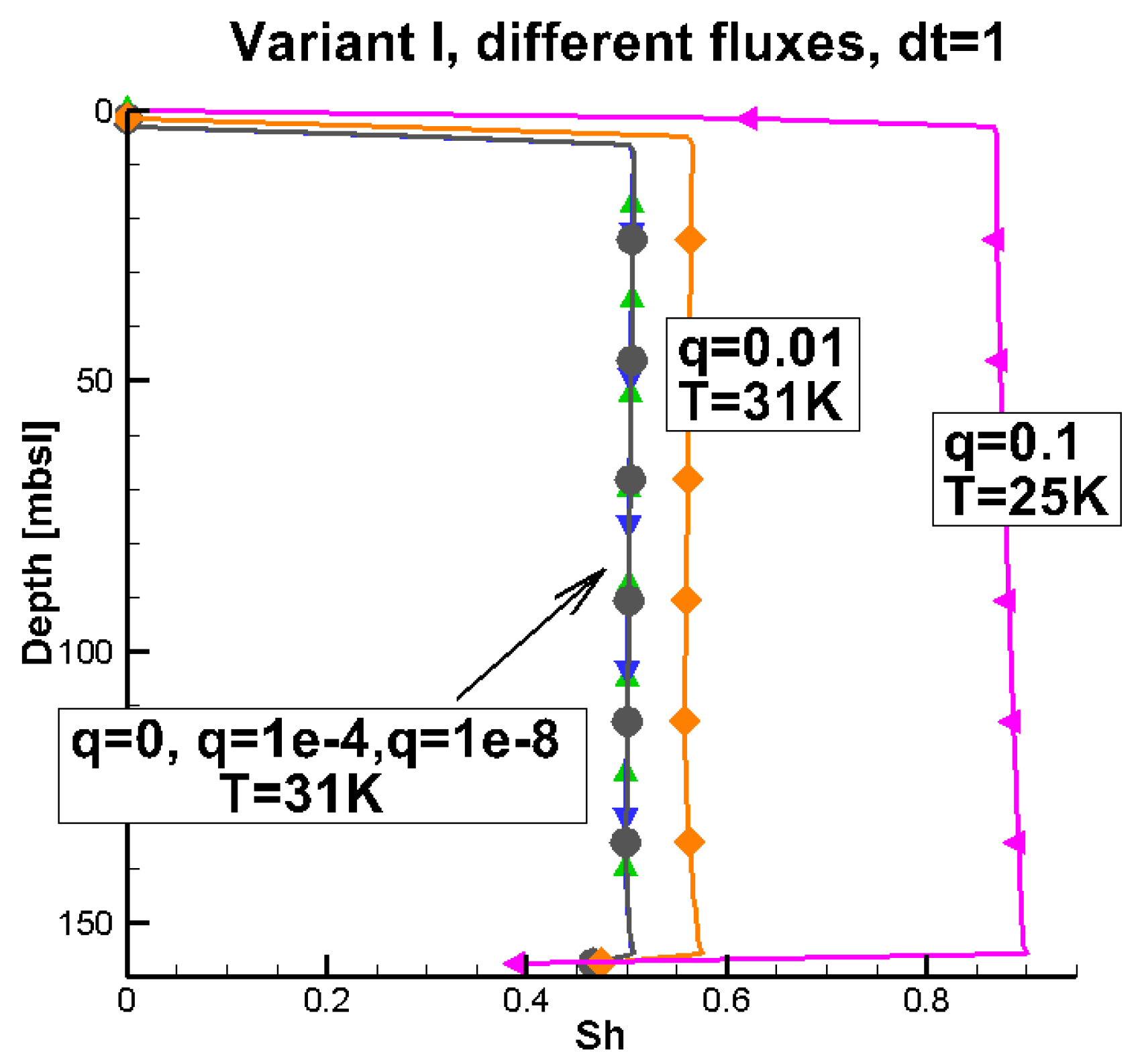
Dependence of the results on q. Next, it is known that the advective fluxes are the hardest physically to handle for hydrate systems, since they provide the source for the fastest hydrate formation.
To test our solvers, we consider the advection-dominated case with large and moderate
q, down to the purely diffusive case with
. In
Figure 4 we present the plots of hydrate saturations at
for different fluxes
q. In addition, in
Table 4 we report the time
when the computational model I predicts that
. We also report the values
and
also for the variants SI and SEQ.
We see that the variants I and SI report essentially the same values. In fact, a close inspection reveals that the model results differ in less than 0.001% between I and SI for the time steps we used in our implementation. This experiment shows again the robustness of all variants with respect to q, with a slight advantage of the implicit variants.
Computational time and the choice of time step. Finally, we evaluate the computational complexity of the variants, and this is done by comparing the wall clock times for our MATLAB implementation. In order to compare the solvers on equal footing, no additional code vectorization is implemented, but the code takes advantage of the natural MATALB vector data types. In
Table 5 we report the wall clock time.
In general, one expects that for the same time step τ the SEQ model is faster than SI and I, since SEQ only uses global linear solvers and local nonlinear flash routines. However, we see that all solvers require similar amounts of computational time, with a slight advantage of model SI. This may be due to the lack of vectorization applied in local flash routines, while the global linear solvers are naturally vectorized in MATLAB. In addition, the SEQ solver computes more local variables than SI and I.
Figure 4.
Hydrate saturation at when different advective fluxes are assumed. For for which high saturation is attained already at we do not show the plot at .
Figure 4.
Hydrate saturation at when different advective fluxes are assumed. For for which high saturation is attained already at we do not show the plot at .
Table 4.
The time T when depending on q, for the base case for each time-stepping variant, respectively, . Here we use .
Table 4.
The time T when depending on q, for the base case for each time-stepping variant, respectively, . Here we use .
| q | | | |
|---|
| 0.1 | 13917 | 13917 | 13972 |
| 0.01 | 27014 | 27014 | 27091 |
| 0.005 | 28629 | 28629 | 28691 |
| 0.0001 | 30568 | 30568 | 30587 |
| 1e−08 | 30614 | 30614 | 30624 |
Since with uniform τ the total computational time scales proportionally to the number of time steps, the choice of τ balances the desired accuracy and computational time. For the case considered here it seems that the time step may be the best practical choice.
The efficiency of the solvers may be very different in 2d or 3d simulations, and we intend to report on these in the future.
Table 5.
Comparison of computational wall clock time for the three model variants and different time steps, for the base case and .
Table 5.
Comparison of computational wall clock time for the three model variants and different time steps, for the base case and .
| τ | | | |
|---|
| 1 | 591.801 | 439.806 | 441.394 |
| 10 | 60.2528 | 44.0688 | 47.6352 |
| 50 | 11.8322 | 8.81442 | 9.63327 |
| 78 | 7.55206 | 5.655 | 6.08011 |
5. Sensitivity to Physical and Coputational Parameters
For a computational model it is crucial to determine what discretization parameters one should use for a given model. In addition, it is important to investigate the sensitivity of the model to the data on
in Equation (
4).
Discretization parameters. As the discretization parameters
and the numbers of cells
and time steps increase, it is expected that the numerical solutions of a PDE model converge to the analytical ones in an appropriate sense dictated by the theoretical numerical analysis. The convergence studies for the purely diffusive one component case of Equation (
3) in [
17] suggest to vary
τ wit
h either linearly or faster, and to consider various metrics of convergence in appropriate functional spaces. For the present case with significant advection
q and variable salinity, we expect the rates to be inferior of the approximate
rates observed in [
17]. The theoretical analysis is underway and will be presented elsewhere.
Here we choose
and the implicit model; in
Figure 5 and
Table 6 we present the evidence which confirms that as
h decreases, the results seem to converge. At the same time it is obvious that the convergence in saturations is quite rough, as observed earlier in [
34].
Figure 5.
Hydrate saturation for different
and
h denoted by dx. See
Table 6 for the related quantitative information extracted from the simulations.
Figure 5.
Hydrate saturation for different
and
h denoted by dx. See
Table 6 for the related quantitative information extracted from the simulations.
Table 6.
Accuracy and complexity of the computational model depending on
, with the time step
τ adjusted to vary linearly with
h. As the quantity of interest depending on
we show the saturation values at
. This table complements the plots in
Figure 5.
Table 6.
Accuracy and complexity of the computational model depending on , with the time step τ adjusted to vary linearly with h. As the quantity of interest depending on we show the saturation values at . This table complements the plots in Figure 5.
| h | τ | | Wall-Clock Time |
|---|
| 10 | 15.9 | 10 | 0.453079 | 5.6533 |
| 25 | 6.36 | 4 | 0.455525 | 32.644 |
| 50 | 3.18 | 2 | 0.459280 | 121.411 |
| 100 | 1.59 | 1 | 0.462181 | 489.101 |
| 200 | 0.795 | 0.5 | 0.465253 | 2301.53 |
The question then is what choice of h and τ balance the conflicting need to decrease the computational time as well as to increase the accuracy, while maintaining an adequate model resolution. From the results presented, we suggest that or corresponding to the discretization in space and in time are a good choice, since they appear to keep the simulation results within the uncertainty envelope that might not be verifiable experimentally.
However, the sensitivity to τ and h at the boundaries needs to be addressed by a more accurate and adaptive formulation especially if nonhomogeneous sediments and/or additional physics are considered.
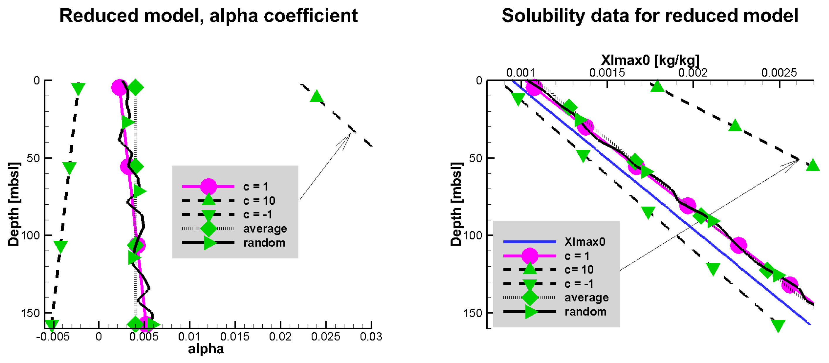
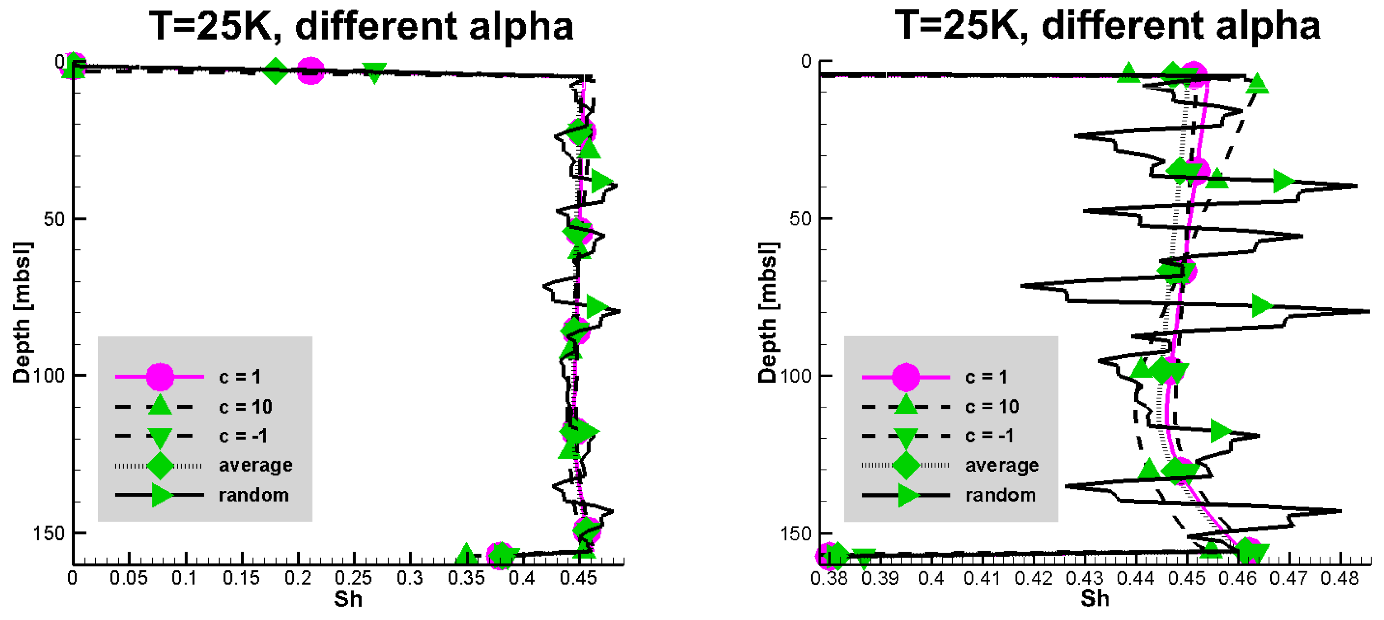
Sensitivity to the parameters of the reduced model Equation (4). There is large uncertainty as to what
one should use. In particular, there may be an error associated with the look-up table process of finding
α described in [
3] and due to the lack of information on salinity. More broadly, in a comprehensive model
depends on the unknown pressure and temperature values, and possibly rock type, thus further variability and uncertainty of
should be expected.
We set up therefore test cases to assess this sensitivity. We dub the values of
obtained for Ulleung Basin in [
3] the “true”
. Next we simulate the hydrate formation with
with
and
. Furthermore, we consider a constant value equal to the average of the true
, and another
which randomly perturbs
. The different cases of
α are shown in
Figure 6, with the corespnding
which we calculated, for illustration purposes, assuming
. In
Figure 7 we show the profiles of
at
coresponding to the different
.
Figure 6.
Parameter
as a function of depth used in
Section 5 (
left) and the corresponding
computed from Equation (
4) and assuming
(
right). On right the plot of
is also shown. The base case from Ulleung Basin [
3] in both plots is denoted with circles. The other cases correspond to
,
, the average of
, and to a randomly perturbed
. The plots for
are out of range and are not fully included.
Figure 7.
Hydrate saturation for different coefficients α. The figure on the (right) is a zoomed in version of that on the (left).
Figure 7.
Hydrate saturation for different coefficients α. The figure on the (right) is a zoomed in version of that on the (left).
Comparing the hydrate saturation for
and
shown in
Figure 7 to the base case with
we see that since
is significantly higher when
, somewhat less hydrate forms. On the other hand, a randomly pertubed
gives
with large local variation, and this is reflected in the corresponding hydrate saturation. This significant sensitivity appears to be of qualitative nature, and requires further studies.
6. Conclusions
In this paper we described the details of the discretization and implementation of a reduced methane hydrate model with variable salinity and significant advection proposed in [
3]. We carried out several convergence and parameter studies to show that the model is robust and computationally sound. Studies of this type have not been provided for the simplified or the comprehensive implicit hydrate models from literature, but are crucial to guide the implementation and to inspire further theoretical and algorithmic developments.
In particular, we defined several time stepping variants: implicit I, semi-implicit SI, and sequential SEQ, which were tested and compared using realistic reservoir data from [
3]. We found, somewhat surprisingly, that the I and SI variants give almost identical results; this may be explained by only a mild dependence of the model on the salinity variable whose treatment differs in I and SI. Furthermore, in the current implementation and 1d test cases there is no significant advantage in one variant over the others as concerns accuracy, robustness, or efficiency. Still, the I model appears as expected somewhat most robust, while SEQ is the easiest to implement by modifying standard advection-diffusion solvers. We also demonstrated the apparent convergence of the solutions when
, and determined practical choices of
. In addition, there is apparent need for grid and model refinement near the boundaries.
Furthermore, we demonstrated the small sensitivity of the reduced thermodynamics model proposed in [
3] to the particular value of the coefficient
α as long as it is qualitatively close to the one from the reservoir data and is monotone. However, a randomly perturbed and nonmonotone
α reveals large sensitivity, and we plan to investigate the reasons further.
Our future work includes theoretical and practical studies of the model convergence as well as its efficiency. There is further need to study additional sets of realistic data and thermodynamics models, and to consider extensions to more complex physical problems.


 ,
, 