Exact Likelihood Calculation under the Infinite Sites Model

Abstract

A key parameter in population genetics is the scaled mutation rate $\theta =4N\mu$, where N is the effective haploid population size and μ is the mutation rate per haplotype per generation. While exact likelihood inference is notoriously difficult in population genetics, we propose a novel approach to compute a first order accurate likelihood of θ that is based on dynamic programming under the infinite sites model without recombination. The parameter θ may be either constant, i.e., time-independent, or time-dependent, which allows for changes of demography and deviations from neutral equilibrium. For time-independent θ, the performance is compared to the approach in Griffiths and Tavaré’s work “Simulating Probability Distributions in the Coalescent” (Theor. Popul. Biol. 1994, 46, 131–159) that is based on importance sampling and implemented in the “genetree” program. Roughly, the proposed method is computationally fast when $n\times \theta <100$, where n is the sample size. For time-dependent $\theta \left(t\right)$, we analyze a simple demographic model with a single change in $\theta \left(t\right)$. In this case, the ancestral and current θ need to be estimated, as well as the time of change. To our knowledge, this is the first accurate computation of a likelihood in the infinite sites model with non-equilibrium demography.

1. Introduction

The infinite sites model is among the simplest models in population genetics. Polymorphism is assumed to arise by single mutations of unique sites along a stretch of DNA. With all mutations occurring at different positions, modeling of genetic variation becomes both mathematically and computationally easier [1]. The infinite sites model thus holds a prominent place in population genetics. Classical studies in this context were based on the Wright-Fisher, the Moran, and the diffusion models (reviewed in, e.g., [2]). Later coalescent theory has been developed. It provides a way to trace the ancestry of a sample backwards in time (reviewed in, e.g., [3]).

The infinite site model can be considered a limiting case of a general model with a finite number of K sites and reversible mutations in the limit of small scaled mutation rates and large K. For such a general model, analytical results are few and computation-intensive methods such as Markov chain Monte Carlo are used for inference (e.g., [4,5]).

The most basic version of the infinite sites model is the so called neutral model. Under equilibrium, i.e., without changes in demography, only one parameter, the scaled mutation rate $\theta =4N\mu$, is needed to characterize the model. Under more complex settings, further parameters are introduced, describing features of demography, selection, and/or recombination. For example, population sizes may vary with time, and consequently scaled mutation rate will also vary. This leads to a time dependent parameter $\theta \left(t\right)=4N\left(t\right)\mu$, and the distribution of the data will deviate from that under neutral equilibrium.

Assuming an infinite sites model without recombination, data can be thought of as arising from a genealogical tree. Depending on the tree and the mutational pattern, many genealogies $\mathcal{T}$ are usually possible for actual data ${\mathcal{D}}^{*}$ . While it is easy to calculate the probability of the data given a specific genealogy and the parameter θ, calculation of the likelihood $Pr\left({\mathcal{D}}^{*}|\theta \right)$ requires summation over all possible genealogies. Hein et al. [2] clearly present the problem in their chapter 2.4 and conclude that there is no “computationally rational way” of summation. Griffiths and Tavaré [6] provide a recursive formula for obtaining the likelihood for small scale problems under neutrality. For larger data sets, however, the algorithm becomes too slow. For such situations, Griffiths and Tavaré [7] propose an importance sampling algorithm (implemented in the program “genetree”). Recently Wu [8] showed that a dynamic programming algorithm can speed up summation over all possible genealogies to make exact calculations feasible for larger datasets. None of these approaches, however, allow for inference in the presence of time-dependent variation of population sizes or mutation rates. The method we propose in this article is applicable beyond these situations. Indeed, we can deal with the above-mentioned scenarios by modeling a time-dependent scaled mutation rate $\theta \left(t\right)$.

In Section 2, we describe our approach and propose an algorithm for constant and a variant algorithm for time dependent parameters. In Section 3, we provide simulation results illustrating efficiency and range of applicability of the method.

2. Dynamic Programming Algorithms for Estimating θ

We first describe a probability model that generates sequence data in our setup. While this model is simple, its direct application does not lead to an efficient computation of the likelihood. We will instead propose a dynamic programming algorithm that permits for an efficient calculation of the likelihood, both for time-independent θ and time-dependent $\theta \left(t\right)$. An equivalent algorithm for the time-independent (but not for the time dependent) case has been proposed by [8].

2.1. Basic Probability Model

We assume an infinite sites model without recombination. A straightforward way to generate samples of n sequences, is to first randomly choose a timed coalescence history with $n-1$ coalescences using a coalescence process with rate parameter $\nu \left(t\right)=1/\left[2N\right(t\left)\right]$ per generation. We note that for small step sizes such a discrete model can also be viewed as an approximation to a continuous time model with exponentially distributed coalescence times.

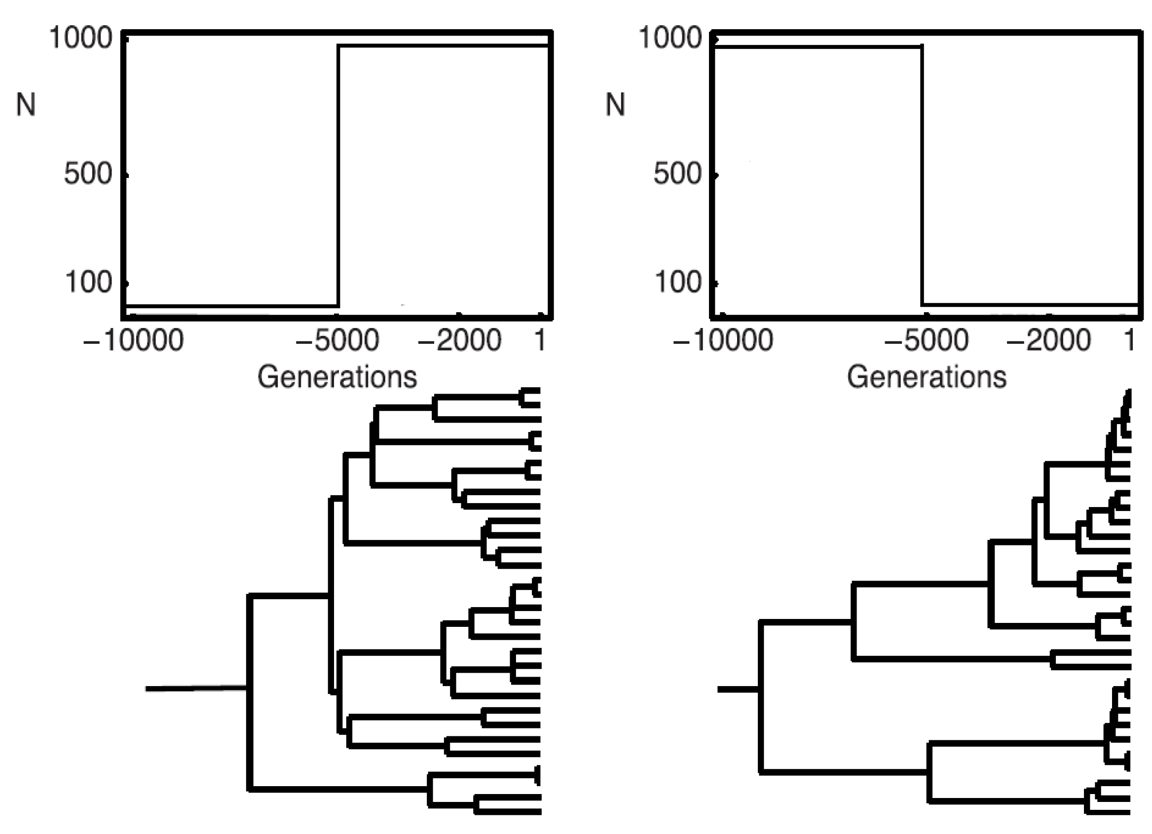
Examples of resulting genealogies are shown in Figure 1. They start from current data and extend to the most recent common ancestor (MRCA) of all sequences in the data. Afterwards, mutations are placed on the coalescence history using a Poisson process with rate μ per sequence and generation (for details see [9]). The number of coalescence events is limited to $n-1$, while the number of mutations is, in principle, unbounded. This model allows for an efficient generation of simulated data, but is inefficient for calculating the likelihood when applied directly.

Figure 1. To the left, a population growing from 10 to 1000 individuals; to the right, a population shrinking from 1000 to 10 individuals; on the top, a schematic graph of the population demographies; on the bottom, a realization of a coalescence tree given the demography.

Figure 1. To the left, a population growing from 10 to 1000 individuals; to the right, a population shrinking from 1000 to 10 individuals; on the top, a schematic graph of the population demographies; on the bottom, a realization of a coalescence tree given the demography.

In more detail, the likelihood is defined as

$$P\left({\mathcal{D}}^{*}\right|\theta )=\sum _{\mathcal{T}}P\left({\mathcal{D}}^{*}\right|\mathcal{T},\theta )P\left(\mathcal{T}\right|\theta )$$

with the sum taken over all possible genealogies with mutations $\mathcal{T}$, and for sequence data ${\mathcal{D}}^{*}$. Notice that a genealogy with mutation defines a unique data set $\mathcal{D}\left(\mathcal{T}\right)$. Thus

$$P\left({\mathcal{D}}^{*}\right|\mathcal{T},\theta )=\left\{\begin{array}{cc}1\hfill & \text{if}\mathcal{D}\left(\mathcal{T}\right)={\mathcal{D}}^{*}\hfill \\ 0\hfill & \text{else}\hfill \end{array}\right.$$

The likelihood can therefore be written as

$$P\left({\mathcal{D}}^{*}\right|\theta )=\sum _{\mathcal{D}\left(\mathcal{T}\right)={\mathcal{D}}^{*}}P\left(\mathcal{T}\right|\theta )$$

(1)

As most genealogies will end in data that differ from the actually observed ones, the direct computation of the likelihood by identifying the genealogies compatible with the data quickly becomes infeasible for larger sample sizes [2].

2.2. Efficient Likelihood Computation

An efficient approach for computing the likelihood can be obtained by recursively identifying the configurations that are compatible with the data, when following their history backwards in time. The feasible trees are then given by the set of all paths from the data to the most recent common ancestor that only use compatible configurations. We will exploit the Markov structure of transitions between configurations to compute the probability of the set of feasible trees recursively. The result of this computation is then the likelihood.

We now explain the proposed approach in more detail. Three scenarios are possible in principle when going backwards in time, from generation $t=i$ to $t=i+1$. Two lineages of ancestry may have coalesced to a single lineage. This occurs, if two identical sequences are both descendants of the same sequence one generation back in time. Alternatively a mutation may have occurred, and a site (DNA nucleotide position) changes its state. The state of the parental sequence in the previous generation is then called ancestral, whereas the new state is called derived. Finally no change may have happened when moving back from generation i to $i+1$.

Let us start supposing that we are at present time ($t=0$) and that our data $\mathcal{D}$ consist of n sequences. Without using the information in the data, any two lines may have coalesced. The probability that any coalescence event occurs is

$$c\left(t\right)=\left(\genfrac{}{}{0pt}{}{n}{2}\right)\nu \left(t\right)+O\left(\nu {\left(t\right)}^2\right)$$

for $t=0$. For sufficiently large populations, $\nu \left(t\right)$ will be small, and the second order term $O\left(\nu {\left(t\right)}^2\right)$ can be ignored with little loss in accuracy. The probability of a mutation event is

$$m\left(t\right)=n\mu \left(t\right)+O\left(\mu {\left(t\right)}^2\right)$$

for $t=0$. For small $\mu \left(t\right)$ the second order term can again be ignored with little loss in accuracy. Finally, the probability of no change from $t=0$ to $t=1$ is $r\left(t\right)=1-c\left(t\right)-m\left(t\right).$

In view of Equation (1), we now investigate the subset of transitions compatible with the data. Recall that polymorphic sites have been caused by mutations on the genealogical tree that connects the data to their root, i.e., the most recent common ancestor. Depending on the tree topology and on where in the tree the mutation occured, specific subsets of sequences will share specific mutations. To summarize this information, the data may be reduced to haplotypes $H^{\left(0\right)}=\{h_1,h_2,\dots ,h_{l_0}\}$, and their corresponding frequencies $U^{\left(0\right)}=(u_1,u_2,\dots ,u_{l_0})$ at generation $t=0$, where $l_0$ is the total number of haplotypes at time $t=0$. Each haplotype is characterised by a unique mutation pattern. We now move one generation backwards in time. If $u_i>1$ for haplotype $h_i$, then $\left(\genfrac{}{}{0pt}{}{u_i}{2}\right)$ coalescence events involving this haplotype are compatible with the data. The new configuration at time $t=1$ resulting from a compatible coalescence event will be

$$\left(H^{\left(0\right)},(u_1,u_2,\dots ,u_{i-1},u_i-1,u_{i+1},\dots ,u_{l_0})\right)$$

Coalescence events between other sequences are not compatible with the data. However, if $u_i=1$, then a mutation may have occured between $t=1$ and $t=0$. (Recall that under the infinite sites model, mutations are impossible for sequences belonging to a haplotype with frequency $u_i>1.$) The contribution to the likelihood by such an event is $q_i\left(t\right)=d_i\mu \left(t\right)+O(\mu {\left(t\right)}^2)$ with $d_i=d_i\left(H\right)$ denoting the number of mutations unique to haplotype $h_i$. If the haplotype without the mutation equals an existing haplotype $h_j$, and for $i<j$ the new configuration will be

$$\left((h_1,h_2,\dots ,h_{i-1},h_{i+1},\dots ,h_{l_0}),(u_1,u_2,\dots ,u_{i-1},u_{i+1},\dots ,u_{j-1},u_j+1,u_{j+1},\dots ,u_{l_0})\right)$$

The case $i>j$ is dealt with analogously. If the new haplotype $h_i^{*}$ is not identical to an existing haplotype, then the new configuration will be

$$\left((h_1,h_2,\dots ,h_{i-1},h_i^{*},h_{i+1},\dots ,h_{l_0}),U^{\left(0\right)}\right)$$

Following common practice, we neglect the possibility of more than one event during a single transition back in time, and omit the second order terms above in our proposed algorithms. Recall that second order terms will have low probability, if both $\mu \left(t\right)$ and $\nu \left(t\right)$ are small.

Whereas there is only one configuration $C^{\left(0\right)}=(H^{\left(0\right)}$, $U^{\left(0\right)})$ at the beginning, there are typically several possible new configurations at subsequent steps. Each coalescence changes the affected haplotype frequency, and each mutation changes the corresponding haplotype. This leads to new configurations in subsequent steps. To obtain all possible intermediate configurations of the data and the transition probabilities, the above procedure needs to be applied starting from each configuration that has positive probability at a given point in time. The identification of configurations compatible with the data can be done recursively. The transitions between subsequent steps form a Markov chain that reaches its absorbing state when only one haplotype remains. The likelihood is given by the sum of all sample path probabilities compatible with the data.

If $\mu \left(t\right)$ and $\nu \left(t\right)$ do not depend on time, the situation simplifies, as the computations can be done conditional on a change. To emphasize that the relevant transition probabilities are constant, we will write $c=c\left(t\right)$, and $r=r\left(t\right)$.

Consider for instance the probability that the next event (whenever in time) will be a coalescence of two sequences sharing haplotype $h_i$:

$$\sum _{j=0}^{\infty }{r}^{j}c=\frac{c}{1-r}$$

This is the conditional probability of the considered coalescence event, given that some change has occurred from $t=1$ to $t=0$. Thus the likelihood computations can be done conditional on the assumption that a change occurred in each step. Let us assume a data set consisting of n sequences with s segregating sites that have arisen from s mutations in the genealogy leading to the sample. Then we will reach the most recent common ancestor (MRCA) after $S=m+s-1$ backward steps that change the configuration. To illustrate the resulting procedure, we present the following simple example.

2.3. Example

Consider a data set with $n=5$ with only one segregating site, i.e., $m=1$: we assume that two identical haplotypes show the ancestral state and three identical haplotypes show the mutation. At step t, we denote the different configurations that are compatible with the data by $c_l^{\left(t\right)}$ with $1\le l\le L\left(t\right).$ As there are only two haplotypes that come up in this example, the configurations can be summarized by the haplotype frequencies $U^{\left(t\right)}=(u_1^{\left(t\right)},u_2^{\left(t\right)})$ of the haplotype $h_1$ without and $h_2$ with the mutation. In our example, the sequence of possible configurations is as follows (Table 1).

Table 1. Haplotype IDs and frequencies in each step of the algorithm.

Step	ID	Haplotype Frequencies $U^{\left(t\right)}$
0	$C^{\left(0\right)}$	(2,3)
1	$C_1^{\left(1\right)}$	(1,3)
1	$C_2^{\left(1\right)}$	(2,2)
2	$C_1^{\left(2\right)}$	(1,2)
2	$C_2^{\left(2\right)}$	(2,1)
3	$C_1^{\left(3\right)}$	(1,1)
3	$C_2^{\left(3\right)}$	(3,0)
4	$C_1^{\left(4\right)}$	(2,0)
5	$C_1^{\left(5\right)}$	(1,0)

Table 1. Haplotype IDs and frequencies in each step of the algorithm.

Step	ID	Haplotype Frequencies $U^{\left(t\right)}$
0	$C^{\left(0\right)}$	(2,3)
1	$C_1^{\left(1\right)}$	(1,3)
1	$C_2^{\left(1\right)}$	(2,2)
2	$C_1^{\left(2\right)}$	(1,2)
2	$C_2^{\left(2\right)}$	(2,1)
3	$C_1^{\left(3\right)}$	(1,1)
3	$C_2^{\left(3\right)}$	(3,0)
4	$C_1^{\left(4\right)}$	(2,0)
5	$C_1^{\left(5\right)}$	(1,0)

As discussed before, we will use first order approximations for the transition probabilities between subsequent states. This also implies that we ignore the case of more than one change in a single step. At time $t=0$, we are in the original configuration, i.e., $X_0=C^{\left(0\right)}$. From $t=0$ to $t=1$, we can move to $C_1^{\left(1\right)}$ or $C_2^{\left(1\right)}$ or stay in the same state. The first move occurs with probability $\left(\genfrac{}{}{0pt}{}{2}{2}\right)·\nu =\nu$, the second with probability $\left(\genfrac{}{}{0pt}{}{3}{2}\right)·\nu =3\nu$. The probability of staying in the same state is $1-\left(\genfrac{}{}{0pt}{}{5}{2}\right)·\nu -5\mu$. The remaining probability is assigned to transitions leading to states incompatible with the data.

The transitions form a Markov chain that will reach the absorbing state $C_1^{\left(5\right)}$ after five steps. The likelihood is given as the sum of the probabilities of all feasible paths ending in $C_1^{\left(5\right)}$.

An equivalent alternative to the dynamic programming algorithm described above has been proposed in [8]. We will now propose a new and more general algorithm that carries over also to more complex demographic models. Consider initially the case when neither ν nor μ depend on time. We can then set $\theta =2\mu /\nu$. For obtaining the MLE it suffices to consider transitions between configurations.

2.4. Calculating the Likelihood for Time-Independent θ

Algorithm 1 Estimating Time-Independent θ

1: Initialization $(t=0)$: Set the configuration at $t=0$ to the data set and its probability to unity, i.e., $f_1^{t=0}=1$. 2: Recursion $(t=1,...,T=m+n-1)$: Generate all configurations compatible with the data that are one step below the current configurations (i.e., have one fewer haplotype or one fewer mutation, but not both), index them by l, with $1\le l\le L\left(t\right)$, for the state t and g, with $1\le g\le L(t+1)$, for the state $(t+1)$ and calculate: $f_l^{(t+1)}={\sum }_g{f}_g^{\left(t\right)}{p}_{gl}^{(t,t+1)}$, where $p_{gl}^{(t,t+1)}=Pr(C_l^{(t+1)}|C_g^{\left(t\right)},\theta )$ are the transition probabilities from state t to $t+1$. 3: Termination: The likelihood is $Pr\left(y|\theta \right)\propto f_1^{\left(T\right)}$.

2.5. Calculating the Likelihood for Time-Dependent θ

Next we consider the case of time-dependent parameters. As both θ and ν depend on the population size N, they vary in particular for populations that grow or shrink over time (see Figure 1).

With a growing population (left hand side in Figure 1), the terminal branches tend to be longer and branches close to the root shorter than under the standard coalescent; with a shrinking population, the opposite holds.

In the case of time-dependence, we not only need to iterate over the transitions between configurations, but also over time. There is no absolute bound on T besides $T<\infty$. According to our simulations however, constraining the time by $T\le 10/\nu$ is usually sufficient for getting accurate approximations. For sufficiently small ν, the approximation to a continuous model is excellent. The following algorithm permits for the inference of parameters under a time dependent demography.

Algorithm 2 Estimating Time-Dependent $\theta (t)$

1: Initialization $(s=0$ and $t=0)$: Set the configuration at $s=0$ and $t=0$ to the data set and its probability to unity, i.e., $f_1^{s=0}(t=0)=1$ and all other variables $f_g^{(s+1)}(t)$ and auxiliary variables $h_1^{s=0}(t)$ to 0. 2: Recursion over time $t=(1,...,T)$ for $s=0$: Generate all configurations compatible with the data that are one step below the current configurations (as above), index them by l, with $1\le l\le L(s=1)$. Set $f_1^{(s=0)}(t)=f_1^{(s=0)}(t-1)p_{11}^{(s=1)}(t-1,t)$, and $h_g^{(s=1)}(t)=f_1(t-1)p_{1g}^{(s=0,s=1)}(t-1,t)$, $p_{ll}^{s=0}=Pr(C_l^{s=0}|C_l^{s=0},\nu ,\mu (t))$ and $p_{lg}^{(s=0,s=1)}=Pr(C_g^{(s=1)}|C_l^{(s=0)},\nu ,\mu (t))$ are the appropriate time-dependent transition probabilities within state $s=0$ and between states $s=0$ and $s=1$. 3: Recursion $s=1,...,S-1$ and $t=1,...,T$: Generate all configurations compatible with the data that are one step below the current configurations (as above), index them by l, with $1\le l\le L(s)$, for the state s, and g, with $1\le g\le L(s+1)$, for the state $(s+1)$. Calculate the functions $f_l^s(t)$ and $h_l^{s+1}(t)$ using: $f_l^s(t)=h_l^s+f_l^s(t-1)p_{ll}^{s,s}(t-1,t)$, $h_g^{s+1}(t)={\sum }_l{f}_l^s(t-1)p_{lg}^{s,s+1}(t-1,t)$, where $p_{ll}^{s,s}=Pr(C_l^s|C_l^s,\nu ,\mu (t))$ and $p_{lg}^{(s,s+1)}=Pr(C_g^{s+1}|C_l^s,\nu ,\mu (t))$ are the appropriate time-dependent transition probabilities within states and between neighboring states. 4: Termination: The likelihood is $Pr\left(y|\theta \right)={\sum }_{t=0}^T{f}_1^{(S)}(t)$.

When only the quotient $\theta \left(t\right)=2\mu \left(t\right)/\nu \left(t\right)$ is of interest, it is sufficient to choose only one of the quantities $\mu \left(t\right)$ and $\nu \left(t\right)$ to be time dependent. To facilitate the choice of a maximum time T, we therefore assumed only $\mu \left(t\right)$ to be time dependent, while ν is assumed constant at all times.

For time dependent parameters, the algorithm needs to run backwards in time, since the time to the most recent common ancestor is unknown. A forward in time algorithm would not work here.

If $\mu \left(t\right)$ and $\nu \left(t\right)$ eventually (i.e., after some generation τ) become constant, the maximum number of steps required will also be bounded. Otherwise some maximum number of steps needs to be introduced. This can be achieved for instance by choosing a maximum number of consecutive iterations without change such that

$$\sum _{j=J}^{\infty }{r}^j=\frac{r^J}{1-r}<ϵ$$

for some desired level of accuracy.

3. Simulations

We simulated scenarios for both time independent and time-dependent θ under an infinite sites model without recombination. For time independent θ, we considered samples of size $n=10$ and 20; $\theta \in 2,4,6$; and $L\in 2,5,10$ independent loci.

For time-dependent θ, we assumed a growing population with one change in the effective population size by a factor of ten at time $0.1\times 4N$. This leads to a current scaled mutation rate ${\theta }_C=2.0$, and an ancestral one of ${\theta }_A=0.2$. We used the ms software [10] to simulate data and wrote a Perl program to convert the ms output into “fasta” format.

Our proposed dynamic programming algorithms provide the likelihood under arbitrary parameter values. To obtain the maximum likelihood estimate, the algorithms needs to be combined with an optimization routine. Here, we used the function Amoeba from Press et al. [11] to find a (local) optimum. This algorithm is relatively slow, but requires few assumptions.

For time independent θ, we compared our dynamic programming (DP) method with the genetree method proposed by Griffiths and Tavaré [7], which is based on importance sampling (see [9,12]). For a single locus, an implementation of this method is available in the genetree software package. We wrote a Perl program to run genetree separately on the L loci, which were considered to be independent, and to combine the obtained likelihoods to an overall likelihood. A C++ implementation of our proposed DP approach is available as supplementary material .

We present simulation results illustrating the accuracy and required computation time of our algorithms. We start with θ constant over time. Here we compare the results of our approach with those obtained using the genetree software. Then we present results for time-dependent $\theta .$

For time-independent θ, the likelihoods calculated with the DP approach are essentially exact, such that any deviations of the genetree estimates indicate numerical inaccuracy of the latter. Under the scenarios addressed in Table 2, the maximum likelihood estimates obtained with genetree remains stable already after a few iterations (in our case ${10}^4$). Indeed, for varying θ the relative likelihood within a run changes only little, but may vary among runs. Compare, e.g., the two runs with ${10}^4$ iterations, where the maximum likelihood location θ is identical, although the estimate of the likelihood of the first run is generally lower than that of the second. Increasing the number of iterations improves the accuracy of the likelihoods, but does not improve the maximum likelihood estimator. In fact, the genetree estimator apparently does often not converge to the DP estimator and thus not to the true maximum likelihood estimator with increasing numbers of iterations.

Table 2. Comparison between log likelihoods calculated with the dynamic programming (DP) method and the with Griffiths and Tavaré (GT) method for a single locus given θ, up to constants. Notice that DP and GT use different normalizations so that the likelihood values are not directly comparable. Instead the values of θ where a maximum is obtained should be compared between methods. The powers of ten in brackets indicate the numbers of iteration. All runs were started with different random number seeds.

θ	DP	GT ($10^4$)	GT ($10^4$)	GT ($10^5$)	GT ($10^6$)	GT ($10^8$)	GT ($10^{10}$)
2.05	−0.7241	2.382	2.604	2.639	2.597	2.595	2.597
2.15	−0.6876	2.431	2.661	2.695	2.652	2.649	2.651
2.25	−0.6602	2.460	2.696	2.730	2.684	2.681	2.684
2.35	−0.6407	2.471	2.710	2.744	2.697	2.694	2.697
2.45	−0.6282	2.465	2.707	2.741	2.693	2.689	2.692
2.55	−0.6219	2.446	2.689	2.722	2.673	2.669	2.671
2.65	−0.6212	2.414	2.656	2.689	2.639	2.635	2.637
2.75	−0.6255	2.372	2.613	2.644	2.594	2.590	2.592
2.85	−0.6342	2.321	2.559	2.589	2.539	2.535	2.537
2.95	−0.6469	2.264	2.497	2.527	2.477	2.473	2.475
3.05	−0.6631	2.200	2.429	2.458	2.408	2.404	2.406

Table 2. Comparison between log likelihoods calculated with the dynamic programming (DP) method and the with Griffiths and Tavaré (GT) method for a single locus given θ, up to constants. Notice that DP and GT use different normalizations so that the likelihood values are not directly comparable. Instead the values of θ where a maximum is obtained should be compared between methods. The powers of ten in brackets indicate the numbers of iteration. All runs were started with different random number seeds.

θ	DP	GT ($10^4$)	GT ($10^4$)	GT ($10^5$)	GT ($10^6$)	GT ($10^8$)	GT ($10^{10}$)
2.05	−0.7241	2.382	2.604	2.639	2.597	2.595	2.597
2.15	−0.6876	2.431	2.661	2.695	2.652	2.649	2.651
2.25	−0.6602	2.460	2.696	2.730	2.684	2.681	2.684
2.35	−0.6407	2.471	2.710	2.744	2.697	2.694	2.697
2.45	−0.6282	2.465	2.707	2.741	2.693	2.689	2.692
2.55	−0.6219	2.446	2.689	2.722	2.673	2.669	2.671
2.65	−0.6212	2.414	2.656	2.689	2.639	2.635	2.637
2.75	−0.6255	2.372	2.613	2.644	2.594	2.590	2.592
2.85	−0.6342	2.321	2.559	2.589	2.539	2.535	2.537
2.95	−0.6469	2.264	2.497	2.527	2.477	2.473	2.475
3.05	−0.6631	2.200	2.429	2.458	2.408	2.404	2.406

Table 3 displays the run times of the DP and the GT approach. If $n\times \theta <100$, where n is the sample size, our method becomes slow.

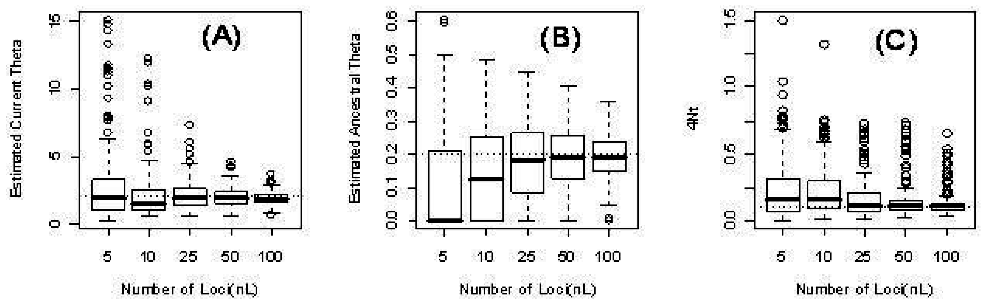
In Table 4, we present results for the case where $\theta \left(t\right)$ is time dependent. The table provides the estimated mean squared error (MSE) for each estimated parameter (i.e., current theta (${\widehat{\theta }}_C$), ancestral theta (${\widehat{\theta }}_A$), time ($\widehat{\tau }$)) based on 1000 simulation runs. As expected, the MSE decreases with the number of independent loci. Figure 2 illustrates the distribution of the parameter estimates.

Figure 2. Three parameters from the time-dependent model for different numbers of loci L: 5, 10, 25, 50, 100. (a) The estimated current scaled mutation rate ${\widehat{\theta }}_C$; (b) The estimated ancestral scaled mutation rate ${\widehat{\theta }}_A$; (c) The estimated time $\widehat{t}$ in units of four times the (effective) population size $4N$.

Figure 2. Three parameters from the time-dependent model for different numbers of loci L: 5, 10, 25, 50, 100. (a) The estimated current scaled mutation rate ${\widehat{\theta }}_C$; (b) The estimated ancestral scaled mutation rate ${\widehat{\theta }}_A$; (c) The estimated time $\widehat{t}$ in units of four times the (effective) population size $4N$.

Table 3. Comparison of run times between maximum likelihood estimates of θ calculated with the dynamic programming (DP) method and the with Griffiths and Tavaré (GT) method for 2, 5, and 10 loci and 10 and 20 haploid individuals. The values stated are the run-times in seconds. All runs were started with different random number seeds.

L	θ	Number	GT ($10^4$)	GT ($10^5$)	GT ($10^6$)	DP
2	2	10	1	4	41	1
		20	1	7	61	9
	4	10	1	6	51	1
		20	1	10	99	41
	6	10	1	8	77	8
		20	2	14	137	153
5	2	10	1	10	100	3
		20	2	18	180	18
	4	10	1	16	103	11
		20	2	22	218	499
	6	10	3	22	233	13
		20	4	35	349	7758
10	2	10	2	21	199	2
		20	5	38	376	114
	4	10	4	32	307	9
		20	6	55	545	3477
	6	10	6	48	471	254
		20	7	62	608	6967

Table 3. Comparison of run times between maximum likelihood estimates of θ calculated with the dynamic programming (DP) method and the with Griffiths and Tavaré (GT) method for 2, 5, and 10 loci and 10 and 20 haploid individuals. The values stated are the run-times in seconds. All runs were started with different random number seeds.

L	θ	Number	GT ($10^4$)	GT ($10^5$)	GT ($10^6$)	DP
2	2	10	1	4	41	1
		20	1	7	61	9
	4	10	1	6	51	1
		20	1	10	99	41
	6	10	1	8	77	8
		20	2	14	137	153
5	2	10	1	10	100	3
		20	2	18	180	18
	4	10	1	16	103	11
		20	2	22	218	499
	6	10	3	22	233	13
		20	4	35	349	7758
10	2	10	2	21	199	2
		20	5	38	376	114
	4	10	4	32	307	9
		20	6	55	545	3477
	6	10	6	48	471	254
		20	7	62	608	6967

Table 4. Mean Squared Error (MSE) of the parameters estimated for a growing population.

No. of Loci	MSE(${\widehat{\theta }}_C$)	MSE(${\widehat{\theta }}_A$)	MSE($\widehat{\tau }$)
5	6.337	0.0392	375.41
10	3.149	0.0254	270.87
25	1.241	0.0133	168.75
50	0.387	0.0080	106.74
100	0.126	0.0040	56.85

Table 4. Mean Squared Error (MSE) of the parameters estimated for a growing population.

No. of Loci	MSE(${\widehat{\theta }}_C$)	MSE(${\widehat{\theta }}_A$)	MSE($\widehat{\tau }$)
5	6.337	0.0392	375.41
10	3.149	0.0254	270.87
25	1.241	0.0133	168.75
50	0.387	0.0080	106.74
100	0.126	0.0040	56.85

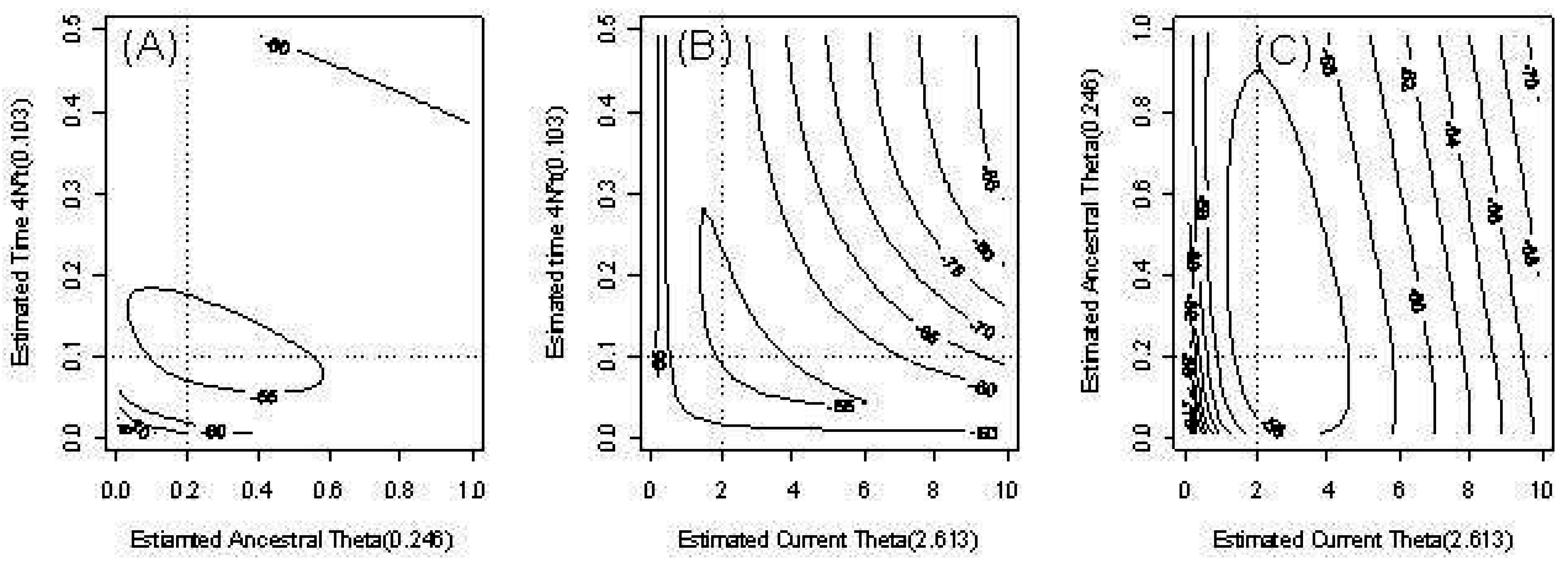
Figure 3 provides an example of the behavior of the estimates of our three parameters in the model with time-dependent θ. We fixed one parameter and provide contour plots of the conditional likelihood of the remaining parameters. The dotted lines indicate the true parameter values. The contours of the likelihood are skewed due to outliers.

Figure 3. Countour plots of the pairwise likelihood of three parameters. (a) The ancestral scaled mutation rate ${\theta }_A$ and time t; (b) The current scaled mutation rate ${\widehat{\theta }}_C$ and time t; (c) The current scaled mutation rate ${\widehat{\theta }}_C$ and ancestral scaled mutation rate ${\theta }_A$.

Figure 3. Countour plots of the pairwise likelihood of three parameters. (a) The ancestral scaled mutation rate ${\theta }_A$ and time t; (b) The current scaled mutation rate ${\widehat{\theta }}_C$ and time t; (c) The current scaled mutation rate ${\widehat{\theta }}_C$ and ancestral scaled mutation rate ${\theta }_A$.

4. Discussion

Under the infinite sites model, we propose a novel method based on dynamic programming for estimating the scaled mutation rate θ. In the case of time-independent θ, the algorithm is similar to that proposed by Wu [8]. Our algorithm however is able to deal with the common situation of a time dependent parameter $\theta \left(t\right)$. Under demographic models, the population size is often assumed to change over time leading to a scaled mutation parameter $\theta \left(t\right)$ that is not constant. As our approach does not include recombination, its use is recommended in cases where the effect of recombination can be neglected. With recombining autosomes, several independent, short loci would be a typical application. Furthermore mitochondrial and chloroplast DNA, as well as non-recombining sex chromosomes also provide suitable settings for our algorithm.

Our proposed method computes the probabilities of all possible configurations at each step. The algorithm is run backwards in time, i.e., from the data to the root. This permits for an extension of the algorithm allowing for time-dependent θ. Here again, exact results can be obtained with realistic datasets.

As expected, our computer simulations confirm that our computed maximum likelihood estimates approach the true parameter values as the number of independent loci increases. See for instance Table 4 and Figure 2) for the more complex case of time-dependent scaled mutation rates. There three parameters are estimated: ancestral and current scaled mutation rates (${\theta }_a$ and ${\theta }_c$), and time of change from the former to the latter.

With our algorithm, it would of course be possible to allow for different functions of time dependence, e.g., exponentially growing or shrinking populations or bottlenecks. For more complex models that involve a larger number of parameters, however, the time required for optimizing the likelihood will increase.

We propose to use our algorithm for small to medium size data sets. It should be pointed out that computation time increases only linearly with the number of independent loci. With increasing scaled mutation rate θ and sample size n, the number of configurations that need to be considered during the likelihood calculations increases. As a rough guideline, the algorithm tends to become slow on a regular desktop computer for $\theta \times n>100$. Notice however that in such large scale problems recombination usually needs to be taken into account, when analyzing autosomal variation. With mitochondria or chloroplast sequences that are not affected by recombination, large datasets are more common. In such situations, approximate algorithms such as importance sampling might be a better choice. With a population genetic model allowing for reversible mutations and a finite number of sites (instead of the infinite sites model) in a Bayesian inference setting, computation-intensive Markov-chain Monte Carlo (MCMC) approaches are available [4,5]. These approaches have often been applied in phylogenetic contexts rather than the population genetic context considered here. Furthermore, it is generally impossible to asses convergence to the posterior distribution with MCMC, such that, usually, convergence to a stationary distribution is assessed instead. In contrast, likelihoods can be calculated essentially exactly with our DP method.