Numerical Solution of the Retrospective Inverse Parabolic Problem on Disjoint Intervals

Abstract

The retrospective inverse problem for evolution equations is formulated as the reconstruction of unknown initial data by a given solution at the final time. We consider the inverse retrospective problem for a one-dimensional parabolic equation in two disconnected intervals with weak solutions in weighted Sobolev spaces. The two solutions are connected with nonstandard interface conditions, and thus this problem is solved in the whole spatial region. Such a problem, as with other inverse problems, is ill-posed, and for its numerical solution, specific techniques have to be used. The direct problem is first discretized by a difference scheme which provides a second order of approximation in space. For the resulting ordinary differential equation system, the positive coerciveness is established. Next, we develop an iterative conjugate gradient method to solve the ill-posed systems of the difference equations, which are obtained after weighted time discretization, of the inverse problem. Test examples with noisy input data are discussed.

1. Introduction

Interface problems have many applications in biology, applied mechanics, heat and mass transfer, etc. [1,2,3,4,5]. Regularity of linear inhomogeneous parabolic interface transmission problems was investigated in [1]. In [2], the author considered two-phase parabolic free boundary problems and established a monotonicity formula for heat functions in disjoint domains. The existence and uniqueness of strong solutions for linear parabolic partial differential equations in two adjoining domains connected through nonlinear Neumann-type interface conditions was studied in [4]. In [5], the advantages of exact representation of the solution in the interface in numerical schemes is discussed.

In this work, we consider a parabolic transmission problem on disjoint domains with exact interface conditions. The derivation of this conditions is discussed in [6,7].

Problems in disjoint domains can be considered a specific instance of interface problems. Mathematically, interface problems result in partial differential equations featuring discontinuities in both the input data and solutions across one or more hypersurfaces with dimensions lower than the domain in which the problem is defined. Different types of conjugation conditions that link domain solutions and their derivatives are known.

The direct parabolic transmission problem in disjoint domains is well studied in the literature. The existence and uniqueness of the weak and strong solutions and the a priori estimate in an appropriate Sobolev-like space were proven in [6,8,9,10,11]. Numerical methods for solving such problems were constructed and analyzed in [8,9,10,11].

Due to many applications in physics, mechanics, biology, finance, etc., a large number of results for inverse problems was obtained in recent decades [12,13,14,15,16,17,18,19,20,21]. As examples of inverse problem applications, we can mention the reconstruction of thermal sources, intensity estimation in the heat transfer, as well as the initial condition estimation based on final time temperature measurements. The backward problem of determination of the initial condition of the direct (forward) problem from a known final time value of the parabolic problem solution is often referred to as a retrospective inverse problem (RIP).

Implementing an inverse source problem for a parabolic transmission problem by using a single measurement on a part of a time interval was considered in [22]. In [23], the authors constructed and analyzed a numerical method for simultaneously determining the initial value and source in a parabolic transmission problem. In [24,25], an inverse boundary value problem for the heat equation in a two-layered medium with unknown inclusions is solved numerically.

In our previous works, we constructed numerical algorithms for solving the parabolic transmission problem in disjoint domains. The inverse problem for reconstruction of a time-dependent source in classical and time-fractional problems from point or integral observations was solved in [26,27], respectively. The inverse problem for identification of external boundary conditions from point measurements was developed and analyzed in [28]. In all these papers, using implicit-explicit time stepping for each time level, the full inverse problem was decoupled into two Dirichlet inverse problems. Then, a decomposition technique or loaded equation method was applied.

The retrospective inverse problem for parabolic equation consists of reconstruction of the unknown initial condition from a given final time observation. It is not well posed, as a small perturbation of the input data can produce large perturbations in the solution (see, for example, [29,30,31,32,33,34,35]). The main difficulty in the construction of a numerical approximation of the solution comes from the strong ill-posedness of the differential problem and the poor conditioning of the corresponding algebraic equations.

To the best of our knowledge, [36] is the first work that studied an RIP numerically. The RIP for heat conduction was solved as an optimal control problem of an object with distributed parameters in [29]. In [31,33,34], the authors constructed an iterative numerical method for the solution of an RIP for one- and multi-dimensional parabolic equations. An efficient numerical method for solving the RIP for a time-fractional parabolic equation was developed in [32]. The authors applied a conjugate gradient-type regularization method to solve the discrete ill-posed linear system. In [37,38], the existence and uniqueness of a quasi-solution to backward time-fractional and space-time-fractional diffusion equations were studied. The Levenberg–Marquardt regularization method was applied to solve the ill-posed problem. A regularization approach for solving the retrospective diffusion problem was also proposed in [30]. In [35], the variation method was utilized for solution of the RIP for a nonlinear, heterogeneous Burgers’ equation. Another important method, at least in terms of theoretical aspects, is the method of regularization of a parabolic equation backward in time through nonlocal initial boundary value problems (see [16] (Section 3.3)) [39]. A disdvantage of this method is the nonlocal initial conditions which arise that require specific numerical techniques.

However, there are no results for the inverse retrospective problem of our type in the case where the governing equations are situated in disconnected domains.

In this paper, we unfold the finite-difference method proposed in [31,33,34] and solve numerically the nonstandard RIP for recovering the initial condition in a parabolic equation in disjoint domains.

The remaining part of this paper is organized as follows. In the next section, we introduce the physical model problem. Section 3 is devoted to the well-posedness of the direct problem in specific weighted Sobolev spaces. In Section 4, we describe the semidiscretization of the direct problem. In Section 5, we describe the iterative method for solving the inverse problem in Equations (1)–(5) and (7)–(9). The stability of the numerical approach is discussed in Section 6. In the next section, we propose our computational results. This paper is finalized in the Conclusions section.

2. Model Problem

In this section, we briefly describe the direct and inverse problems for our physical model.

We focus on the following transmission problem in a disconnected domain [6,9]:

$$\begin{array}{ccc}& & \frac{\partial u_j}{\partial t}+L_j\left(u\right)=f_j(x,t),(x,t)\in Q_j={\Omega }_j\times (0,T],j=1,2,\hfill \\ & & L_j\left(u\right)=-\frac{\partial }{\partial x}\left(p_j(x,t)\frac{\partial u_j}{\partial x}\right)+q_j(x,t)u_j,\hfill \\ & & {\Omega }_j=(a_j,b_j),-\infty <a_1<b_1<a_2<b_2<+\infty ,\hfill \end{array}$$

(1)

with the interface conditions

$$\begin{array}{ccc}& & p_1(b_1,t)\frac{\partial u_1}{\partial x}(b_1,t)+{\alpha }_1{u}_1(b_1,t)={\beta }_1{u}_2(a_2,t)+{\gamma }_1\left(t\right),t\in (0,T),\hfill \end{array}$$

(2)

$$\begin{array}{ccc}\hfill -& & p_2(a_2,t)\frac{\partial u_2}{\partial x}(a_2,t)+{\alpha }_2{u}_2(a_2,t)={\beta }_2{u}_1(b_1,t)+{\gamma }_2\left(t\right),t\in (0,T),\hfill \end{array}$$

(3)

as well as the external boundary conditions

$$\begin{array}{ccc}& & u_1(a_1,t)={\phi }_1\left(t\right),t\in (0,T),\hfill \end{array}$$

(4)

$$\begin{array}{ccc}& & u_2(b_2,t)={\phi }_2\left(t\right),t\in (0,T),\hfill \end{array}$$

(5)

and the initial conditions

$$u_j(x,0)=u_j^{\circ }\left(x\right),x\in {\overline{\Omega }}_j=[a_j,b_j].$$

(6)

Furthermore, with a small modification, concerning the time dependence of the diffusion and reaction coefficients, we follow the results in [6,9], assuming that

$$\begin{array}{c}\hfill \begin{array}{cc}\hfill & {\displaystyle p_j\in H^{2+\epsilon ,1+\epsilon /2}\left(Q_j\right),q_j\in H^{1+\epsilon ,(1+\epsilon )/2}\left(Q_j\right),{\gamma }_j\left(t\right)\in H^{1/2}(0,T),}\hfill \\ & {\displaystyle f_j(x,t)\in L^{1,1/2}\left(Q_j\right),p_j(x,t)\ge p_{j_0}>0,q_j(x,t)\ge 0,j=1,2,}\hfill \end{array}\end{array}$$

(7)

$${\beta }_j>0,{\alpha }_j>0,j=1,2,{\beta }_1{\beta }_2<{\alpha }_1{\alpha }_2,$$

(8)

where $H^{\mu ,\nu }$ are traditional Sobolev spaces (see, for example, [40,41,42]).

When all coefficients and right-hand sides in Equation (1) are known, and the boundary conditions in Equations (2)–(5) and the initial conditions in Equation (6) are given, this problem is called a direct or forward problem.

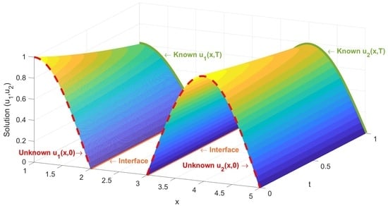
The retrospective inverse problem for the system in Equations (1)–(6) consists of the recovery of an a priory unknown initial state (Equation (6)) and the solution $u(x,t)=\{u_1(x,t),u_2(x,t)\}$, $0\le t\le T$ with the known observations at the final time:

$$u_j(x,T)={\varphi }_j\left(x\right),j=1,2.$$

(9)

The sense of the simple model, described by the system in Equations (1)–(9), is heat conduction into interacted one-dimensional rods of lengths $b_j-a_j$ ($j=1,2$) whose temperature at point x and time t is modeled by the functions $u_j(x,t)$ ($j=1,2$), which solves Equation (1). The left end of the first rod and the right end of the second rod are isolated if ${\phi }_1\left(t\right)={\phi }_2\left(t\right)=0$ in Equatons (4) and (5) and retain the temperature otherwise. Next, there is a heat exchange between the rods described by the conditions in Equations (2) and (3). The initial temperature (Equation (6)) of the rods is unknown. It is required to reconstruct the functions $u_j^{\circ }$ ($j=1,2$) from the measured temperatures ${\varphi }_j\left(x\right)$ ($j=1,2$) at $t=T$.

There are several papers on similar parabolic problems with nonlocal interface conditions and their physical approximations (see, for example, [2,3,4,5]).

3. Well-Posedness of the Direct Problem

In this section, we present the results for the existence and uniqueness of a strong solution to the problem in Equations (1)–(6) as obtained in [8]. However, by assuming more smoothness (Equation (7)), in comparison with [8], we obtain a smooth solution $u=\{u_1,u_2\}$ to the differential problem in Equations (1)–(6). Our main concern is the coerciveness of the bilinear form A. This property will be used in the construction of the iterative algorithm.

We consider the product space

$$L=L_2\left({\Omega }_1\right)\times L_2\left({\Omega }_2\right)=\{v=(v_1,v_2)|v_j\in L_2\left({\Omega }_j\right)\},$$

equipped with the inner product and norm

$${(u,v)}_L={\beta }_2{(v_1,v_1)}_{L_2\left({\Omega }_1\right)}+{\beta }_1{(v_2,v_2)}_{L_2\left({\Omega }_2\right)},\parallel v\parallel ={(v,v)}_L^{1/2},$$

where

$${(u_j,v_j)}_{L_2\left({\Omega }_j\right)}=\underset{{\Omega }_j}{\int }{u}_j{v}_{j}dx,j=1,2.$$

In addition, we introduce the space

$$H^k=\{v=(v_1,v_2)|v_j\in H^k\left({\Omega }_j\right)\},k=1,2,\dots$$

equipped with the following inner product and norm:

$${(u,v)}_{H^k}={\beta }_2{(v_1,v_1)}_{H^k\left({\Omega }_1\right)}+{\beta }_1{(v_2,v_2)}_{H^k\left({\Omega }_2\right)},{\parallel v\parallel }_{H^k}={(v,v)}_{H^k}^{1/2},$$

where

$${(u_j,v_j)}_{H^k\left({\Omega }_j\right)}=\sum _{s=0}^k{\left(\frac{d^s{u}_j}{d{x}^j},\frac{d^s{v}_j}{d{x}^j}\right)}_{L_2\left({\Omega }_s\right)},j=1,2,k=1,2,\dots$$

Specifically, we assign

$$H_0^2=\{v=(v_1,v_2)\in H^2|v_1\left(a_1\right)={\phi }_1\left(t\right),v_2\left(b_2\right)={\phi }_2\left(t\right)\},k=1,2,\dots$$

We introduce the bilinear form corresponding to the problem in Equations (1)–(6):

$$\begin{array}{ccc}\hfill A(u,v)& =& {\beta }_2\underset{{\Omega }_1}{\int }{p}_1\frac{d{u}_1}{d{x}_1}\frac{d{v}_1}{d{x}_1}dx+{\beta }_1\underset{{\Omega }_2}{\int }{p}_2\frac{d{u}_2}{d{x}_2}\frac{d{v}_2}{d{x}_2}dx\hfill \\ & & +{\beta }_2{\alpha }_1{v}_1\left(b_1\right)w_1\left(b_1\right)+{\beta }_1{\alpha }_2{v}_2\left(a_2\right)w_2\left(a_2\right)-{\beta }_1{\beta }_2\left[v_1\left(b_1\right)w_2\left(a_2\right)+v_2\left(a_2\right)w_1\left(b_1\right)\right].\hfill \end{array}$$

(10)

On the base of the results in [8,9], we establish the following statements:

Lemma 1.

Under the conditions in Equations(7) and (8), the bilinear form A, defined by Equation (10), is symmetric and bounded on $H^2\times H^2$. Moreover, this form is also coercive on $H_0^2$ (i.e., there exists a constant $c_0>0$ such that $A(v,v)\ge c_0{\parallel \parallel }_{H^2}^2$ for all $v\in H_0^2$).

Let $u\left(t\right)$ be a function mapping $\Omega \in {\mathbb{R}}^n$ into a Hilbert space H. Furthermore, we define [40] the Sobolev space $H^k(\Omega ,H)$ with an inner product

$${(u,v)}_{H^k(\Omega ,H)}=\underset{\Omega }{\int }\sum _{\alpha \le k}\left(D^{\alpha }u\left(t\right),D^{\alpha }v\left(t\right)\right),$$

where k in a non-integer. For $k=0$, we set $L_2(\Omega ,H)=H^0(\Omega ,H)$.

Next, we introduce the space $H^{k,k/2}=L_2\left((0,T),H^k\right)\cap H^{k/2}\left((0,T),L\right)$.

Theorem 1.

Let the assumptions in Equations (7) and (8) hold and $u_0=(u_{10},u_{20})\in H_0^1$. Then, the initial boundary value problem in Equations (1)–(6) has a unique strong solution $u=(u_1,u_2)\in H^{2,1}$, and the following a priory estimate holds true

$${\parallel u\parallel }_{H^{2,1}}^2\le C\sum _{j=1}^2{\beta }_{3-j}\left({\parallel u_{j0}\parallel }_{H^1\left({\Omega }_j\right)}^2+{\parallel f_j\parallel }_{H^{1,1/2}\left(Q_j\right)}^2+{\parallel {\gamma }_j\parallel }_{H^{1/2}(0,T)}^2\right).$$

Let us note that the increase in the smoothness of the input data leads to the increase in the solution’s smoothness. Furthermore, using this fact, we assume that the sufficient smoothness of the differential problem’s solution requires the construction of corresponding difference schemes.

4. Semidiscrerization of the Direct Problem

First, we a construct finite difference scheme for the direct problem in Equations (1)–(6). We introduce a uniform partition of the intervals ${\Omega }_j$ through meshes ${\overline{\omega }}_{h_j}$ ($j=1,2$):

$${\overline{\omega }}_{h_j}=\{x_{j,i_j}:x_{j,i_j}=a_j+i_j{h}_j,i_j=0,1,\dots ,N_j,h_j=(b_j-a_j)/N_j\},j=1,2$$

We also denote the mesh function $y_j(x,t)$ at node $(x_{j,i_j},t)$ by $y_{i,j_i}\left(t\right)=y_{i,j_i}$. Next, we also introduce the notations

$$\begin{array}{cc}& {\displaystyle y_{j,x_{i_j}}=\frac{y_{j,i_j+1}-y_{j,i_j}}{h_j},y_{j,{\overline{x}}_{i_j}}=\frac{y_{j,i_j}-y_{j,i_j-1}}{h_j},a_{j,i_j}=p_{j,i_j-1/2}=p_j(x_{j,i_j}-h_j/2,t),}\\ & {\displaystyle \langle y_j,w_j\rangle =\sum _{i_j=0}^{N_j}{h}_j{y}_{j,i_j}{w}_{j,i_j},\parallel y\parallel =\sqrt{\langle y_j,y_j\rangle }.}\end{array}$$

By applying the finite-volume method and eliminating the external boundary grid nodes $x_{1,0}=a_1$, $x_{2,N_2}=b_2$, we obtain the spatial semidiscretization of Equations (1)–(6):

$$\begin{array}{ccc}& & \frac{d{u}_{j,i_j}}{dt}+{\mathcal{L}}_j\left(u_{j,i_j}\right)=g_{j,i_j},j=1,2,i_1=1,\dots ,N_1,i_2=0,\dots ,N_2-1,\hfill \\ & & \mathrm{or}{i}_j=2-j,3-j,\dots ,N_j-j+1,\hfill \end{array}$$

(11)

where

$$\begin{array}{ccc}& & {\mathcal{L}}_j\left(u_{j,i_j}\left(t\right)\right)={\mathcal{L}}_j\left(u_{j,i_j}\right)=q_{j,i_j}{u}_{j,i_j}\hfill \\ & & -\frac{1}{h_j}\left\{\begin{array}{cc}{\displaystyle a_{j,i_j+1}{u}_{j,x_{i_j}}-a_{j,i_j}{u}_{j,{\overline{x}}_{i_j}},}\hfill & i_j=3-j,4-j,\dots ,N_j-j,\hfill \\ {\displaystyle a_{1,2}{u}_{1,x_1}-a_{1,1}\frac{u_{1,1}}{h_1},}\hfill & j=1,i_1=1,\hfill \\ {\displaystyle -{\alpha }_1{u}_{1,N_1}+{\beta }_1{u}_{2,0}-a_{1,N_1}{u}_{1,{\overline{x}}_{N_1}},}\hfill & j=1,i_1=N_1,\hfill \\ {\displaystyle a_{2,1}{u}_{2,x_0}-{\alpha }_2{u}_{2,0}+{\beta }_2{u}_{1,N_1},}\hfill & j=2,i_2=0,\hfill \\ {\displaystyle -a_{2,N_2}\frac{u_{2,N_2-1}}{h_2}-a_{2,N_2-1}{u}_{2,{\overline{x}}_{N_2-1}},}\hfill & j=2,i_2=N_2-1,\hfill \end{array}\right.\hfill \\ & & g_{j,i_j}=\left\{\begin{array}{cc}{\displaystyle f_{j,i_j}\left(t\right),}\hfill & i_j=2,3,\dots ,N_j-2,\hfill \\ {\displaystyle f_{1,1}\left(t\right)+a_{1,1}\frac{{\phi }_1\left(t\right)}{h_1^2},}\hfill & j=1,i_1=1,\hfill \\ {\displaystyle \frac{1}{2}{f}_{1,N_1}\left(t\right)+\frac{{\gamma }_1\left(t\right)}{h_1},}\hfill & j=1,i_1=N_1,\hfill \\ {\displaystyle \frac{1}{2}{f}_{2,0}\left(t\right)+\frac{{\gamma }_2\left(t\right)}{h_2},}\hfill & j=2,i_2=0.\hfill \\ {\displaystyle f_{2,N_2-1}\left(t\right)+a_{2,N_2}\frac{{\phi }_2\left(t\right)}{h_2^2},}\hfill & j=2,i_2=N_2-1.\hfill \end{array}\right.\hfill \end{array}$$

Furthermore, for convenience, we rearrange the indexes, representing the unknown solution and corresponding functions in the form $U_i=(u_{1,i_1},u_{2,i_2})$, $G_i=(g_{1,i_1},g_{2,i_2})$, $i_1=1,2,\dots ,N_1$, $i_2=0,1,\dots ,N_2-1$, $i=1,2,\dots ,N$, $N=N_1+N_2$. With these notations, the full discrete scheme in Equation (11) is rewritten as follows:

$$\frac{d{U}_i}{dt}+{\mathcal{L}}_i\left(U_i\right)=G_i,i=1,\dots ,N,$$

(12)

where

$$\mathcal{L}=\left[\begin{array}{cc}{A}_1& O_1,\\ O_2& A_1\end{array}\right],$$

and

$$A_1=\frac{1}{h_1^2}\left[\begin{array}{ccccccc}{a}_{1,1}+a_{1,2}& -a_{1,2}& 0& 0& \dots & 0& 0\\ -a_{1,2}& a_{1,2}+a_{1,3}& -a_{1,3}& 0& \dots & 0& 0\\ 0& -a_{1,3}& a_{1,3}+a_{1,4}& -a_{1,4}& \dots & 0& 0\\ \dots \dots \dots \\ 0& 0& 0& 0& \dots & -a_{1,N_1}& a_{1,N_1}+{\alpha }_1{h}_1\end{array}\right],$$

$$A_2=\frac{1}{h_2^2}\left[\begin{array}{ccccccc}{a}_{2,1}+{\alpha }_2{h}_2& -a_{2,1}& 0& 0& \dots & 0& 0\\ -a_{2,1}& a_{2,1}+a_{2,2}& -a_{2,2}& 0& \dots & 0& 0\\ 0& -a_{2,3}& a_{2,2}+a_{2,3}& -a_{2,3}& \dots & 0& 0\\ \dots \dots \dots \\ 0& 0& 0& 0& \dots & -a_{2,N_2-1}& a_{2,N_2-1}+a_{2,N_2}\end{array}\right],$$

$$O_1=\frac{1}{h_1}\left[\begin{array}{cccccc}0& 0& 0& \dots & 0& 0\\ 0& 0& 0& \dots & 0& 0\\ \dots & \dots & \dots \\ 0& 0& 0& \dots & 0& 0\\ -{\beta }_1& 0& 0& \dots & 0& 0\end{array}\right],O_2=\frac{1}{h_2}\left[\begin{array}{cccccc}0& 0& 0& \dots & 0& -{\beta }_2\\ 0& 0& 0& \dots & 0& 0\\ \dots & \dots & \dots \\ 0& 0& 0& \dots & 0& 0\\ 0& 0& 0& \dots & 0& 0\end{array}\right].$$

In this framework, the scalar product and the corresponding norm are defined as follows:

$$\langle Y,W\rangle =\sum _{i=1}^{N_1}{h}_1{Y}_i{W}_i+\sum _{i=N_1+1}^N{h}_2{Y}_i{W}_i,\parallel Y\parallel =\sqrt{\langle Y,Y\rangle }.$$

Considering the main goal of the present research, namely the numerical solution of the retrospective problem in Equations (1)–(5), (7) and (9), the following results are of basic importance:

Lemma 2.

Let $u(x,t)=\{u_1(x,t),u_2(x,t)\}$ be $C^2$-smooth in the space solution to the problem in Equations (1)–(8) and $\left\{U_i\left(t\right)\right\}$ be the solution to the discrete problem in Equation (12). Then, the operator $\mathcal{L}$ is positively definite, and the difference scheme is of the second order of approximation.

Proof. 

The second order of approximation directly follows from the construction of Equation (11).

Next, we multiply the first $N_1$ number of equations in Equation (12) by ${\beta }_2$ and the remaining $N_2$ number of equations by ${\beta }_1$, and in the resulting discrete system, we set

$$\tilde{\mathcal{L}}=\left[\begin{array}{cc}{\beta }_2& 0\\ 0& {\beta }_1\end{array}\right]\mathcal{L}.$$

Taking into account that $U_i=(u_{1,i_1},u_{2,i_2})$, $i_1=1,2,\dots ,N_1$, $i_2=0,1,\dots ,N_2-1$, $i=1,2,\dots ,N$, we consider

$$\begin{array}{ccc}\hfill \langle U,\tilde{\mathcal{L}}\left(U\right)\rangle & =& {(U,\mathcal{L}\left(U\right))}_L=\frac{{\beta }_2}{h_1}\left(a_{1,1}{u}_{1,1}^2+\sum _{i=1}^{N_1-1}{a}_{1,i+1}{(u_{1,i+1}-u_{1,i})}^2\right)\hfill \\ & & +\frac{{\beta }_1}{h_2}\left(a_{2,N_2+1}{u}_{2,N_2}^2+\sum _{i=0}^{N_2-1}{a}_{2,i+1}{(u_{2,i+1}-u_{2,i})}^2\right)\hfill \\ & & +{\alpha }_1{\beta }_2{u}_{1,N_1}^2-2{\beta }_1{\beta }_2{u}_{1,N_1}{u}_{2,0}+{\alpha }_2{\beta }_1{u}_{2,0}^2\hfill \\ & \ge & {C\parallel U\parallel }^2+{\alpha }_1{\beta }_2\left({\left(u_{1,N_1}-\frac{{\beta }_1}{{\alpha }_1}{u}_{2,0}\right)}^2+\frac{{\beta }_1}{{\alpha }_1}\left(\frac{{\alpha }_2}{{\beta }_2}-\frac{{\beta }_1}{{\alpha }_1}\right)u_{2,0}^2\right)\hfill \end{array}$$

Therefore, under the conditions in Equation (8), we obtain

$$\langle U,\tilde{\mathcal{L}}\left(U\right)\rangle \ge C{\parallel U\parallel }^2,$$

where C is a positive constant.    □

Let us note that from the definiteness (i.e., the coerciveness of the operator $\mathcal{L}$), the solution to the energy stability for the ODEs (Equation (11)) and its global existence directly follow.

5. Iterative Solution to the Inverse Problem

Now, we consider the uniform temporal mesh

$${\overline{\omega }}_{\tau }=\{t_n:t_n=n\tau ,n=0,1,\dots ,M,\tau =T/M\},$$

such that the computational domain ${{\overline{Q}}_j}_T={\Omega }_j\times [0,T]$ is discretized by a rectangular grid ${\overline{\omega }}_{h_j}\times {\omega }_{\tau }$ ($j=1,2$). The mesh function $y_j(x,t)$ at node $(x_{j,i_j},t_n)$ is denoted by $y_{i,j_i}^n$. Furthermore, the $\sigma$-weighted time stepping ($0<\sigma \le 1$) leads to the following full discrete scheme:

$$\begin{array}{cc}\hfill & \frac{u_{j,i_j}^{n+1}-u_{j,i_j}^n}{\tau }+{\mathcal{L}}_j^{n+\sigma }\left(\sigma u_{j,i_j}^{n+1}+(1-\sigma )u_{j,i_j}^n\right)=g_{j,i_j}^{n+\sigma }\hfill \\ \hfill & u_{j,i_j}^0=u_j^{\circ }\left(x_{j,i_j}\right),j=1,2,i_j=2-j,3-j,\dots ,N_j-j+1,\hfill \end{array}$$

(13)

where ${\mathcal{L}}_j^{n+\sigma }\left(y\right)={\mathcal{L}}_j\left(y,\sigma t_{n+1}+(1-\sigma )t_n\right)$, $g_{j,i_j}^{n+\sigma }=g_{j,i_j}(t_{n+1}+(1-\sigma )t_n)$.

As before, we rearrange the indexes, where the unknown solution and corresponding functions are $U_i^n=U_i\left(t_n\right)$, $G_i^n=G_i\left(t_n\right)$, ${\overline{a}}_i^n=(a_{1,i_1}^n,a_{2,i_2}^n)$, ${\overline{q}}_i^n=(q_{1,i_1}^n,q_{2,i_2}^n)$, ${\overline{f}}_i^n=(f_{1,i_1}^n,f_{2,i_2}^n)$, $i=1,2,\dots ,N$, $i_1=1,2,\dots ,N_1$, $i_2=0,1,\dots ,N_2-1$. With these notations, the full discrete scheme (Equation (13)) is rewritten as follows:

$$\begin{array}{cc}\hfill & \frac{U_i^{n+1}-U_i^n}{\tau }+{\mathcal{L}}_i^{n+\sigma }\left(\sigma U_i^{n+1}+(1-\sigma )U_i^n\right)=G_i^{n+\sigma },\hfill \\ \hfill & U_i^0=u_i^{\circ },i=1,2,\dots ,N,\hfill \end{array}$$

(14)

where

$$\begin{array}{ccc}& & {\mathcal{L}}_i^{n+\sigma }\left(Y_i\right)=q_{j,i_j}^{n+\sigma }\left(Y_i\right)\hfill \\ & & -\frac{1}{h_j}\left\{\begin{array}{cc}{\displaystyle {\overline{a}}_{i+1}^{n+\sigma }{Y}_{x_i}-{\overline{a}}_i^{n+\sigma }{Y}_{{\overline{x}}_i},}\hfill & i=2,3,\dots ,N_1-1,N_1+2,\dots ,N-1,\hfill \\ {\displaystyle {\overline{a}}_2{Y}_{x_1}-\frac{{\overline{a}}_1}{h_1}{Y}_1,}\hfill & i=1,\hfill \\ {\displaystyle -{\alpha }_1{Y}_{N_1}+{\beta }_1{Y}_{N_1+1}-{\overline{a}}_{N_1}{Y}_{{\overline{x}}_{N_1}},}\hfill & i=N_1,\hfill \\ {\displaystyle {\overline{a}}_{N_1+2}{Y}_{N_1+1}-{\alpha }_2{Y}_{N_1+1}+{\beta }_2{Y}_{N_1},}\hfill & i=N_1+1,\hfill \\ {\displaystyle -{\overline{a}}_{N_1+N_2+1}\frac{Y_{N-1}}{h_2}-{\overline{a}}_N{Y}_{{\overline{x}}_{N_1+N_2}},}\hfill & i=N.\hfill \end{array}\right.\hfill \\ & & G_i^{n+\sigma }=\left\{\begin{array}{cc}{\displaystyle {\overline{f}}_i^{n+\sigma },}\hfill & i=2,3,\dots ,N_1-1,N_1+2,\dots ,N-1,\hfill \\ {\displaystyle {\overline{f}}_1^{n+\sigma }+a_1^{n+\sigma }\frac{{\phi }_1^{n+\sigma }}{h_1^2},}\hfill & i=1,\hfill \\ {\displaystyle \frac{1}{2}{\overline{f}}_{N_1}^{n+\sigma }+\frac{{\gamma }_1^{n+\sigma }}{h_1},}\hfill & i=N_1,\hfill \\ {\displaystyle \frac{1}{2}{\overline{f}}_{N_1+1}^{n+\sigma }+\frac{{\gamma }_2^{n+\sigma }}{h_2},}\hfill & i=N_1+1.\hfill \\ {\displaystyle {\overline{f}}_N^{n+\sigma }+{\overline{a}}_{N+1}\frac{{\phi }_2^{n+\sigma }}{h_2^2},}\hfill & i=N,\hfill \end{array}\right.\hfill \end{array}$$

In order to solve the inverse problem in Equations (1)–(5) and (9) for reconstruction of the initial conditions (Equation (6)), we consider the discretization in Equation (13) (or Equation (14)) associated with Equation (9), namely

$$U_i^M={\varphi }_i,i=1,2,\dots ,N.$$

Let E be the unit matrix of a size $N\times N$ and introduce the notations

$$D^{n+\sigma }={[E+\sigma \tau {\mathcal{L}}^{n+\sigma }]}^{-1},S^{n+\sigma }=D^{n+\sigma }[E+(\sigma -1)\tau {\mathcal{L}}^{n+\sigma }].$$

Thus, from Equation (14), for the solution vector $U^n=[U_1^n,U_2^n,\dots ,U_N^n]$ at a new time level, we have

$$U^{n+1}=S^{n+\sigma }{U}^n+\tau D^{n+\sigma }{G}^{n+\sigma }.$$

(15)

Consequently, after time integration, from Equation (15), we obtain

$$U^{n+1}=\prod _{k=0}^n{S}^{k+\sigma }{U}^0+\tau \sum _{k=0}^n{D}^{k+\sigma }{B}^{k+\sigma }{G}^{k+\sigma },$$

(16)

where

$$B^{k+\sigma }=\left\{\begin{array}{cc}{\displaystyle \prod _{j=k+1}^n}{S}^{j+\sigma },\hfill & k+1\le n,\hfill \\ E,\hfill & k+1>n.\hfill \end{array}\right.$$

Therefore, for $n=M-1$, from Equation (16) we obtain

$$\Phi =\prod _{k=0}^{M-1}{S}^{k+\sigma }{U}^0+\tau \sum _{k=0}^{M-1}{D}^{k+\sigma }{B}^{k+\sigma }{G}^{k+\sigma },$$

(17)

where $\Phi =({\varphi }_1,{\varphi }_2)=[\varphi \left(x_{1,1}\right),\varphi \left(x_{1,2}\right),\dots ,\varphi \left(x_{1,N_1}\right),\varphi \left(x_{2,0}\right),\varphi \left(x_{2,1}\right),\dots ,\varphi \left(x_{2,N_2-1}\right)]$.

Finally, the initial condition is determined by solving the linear equation

$$\prod _{k=0}^{M-1}{S}^{k+\sigma }{U}^0=\Phi -\tau \sum _{k=0}^{M-1}{D}^{k+\sigma }{B}^{k+\sigma }{G}^{k+\sigma }.$$

(18)

Since the operator $S^{n+\sigma }$, $n=0,1,\dots ,M-1$ is self-adjoint, and $S^{n+\sigma }={\left(S^{n+\sigma }\right)}^{\ast }$ and is positive, it follows from Lemma 2 that its inverse exists and is also self-adjoint and positive. Consequently, for the solution of the system of linear algebraic Equation (18) with a full coefficient matrix, it is appropriate to use the conjugate gradient method (CGM). The steps are described in Algorithm 1.

Algorithm 1 CGM for solving an RIP.

Require: ${\varphi }_j\left(x\right)$, $j=1,2$, initial guess $V_0$ for $U^0$, consistent with external boundary conditions, accuracy $\epsilon >0$

Ensure: $U^n$, $n=0,1,\dots ,M-1$     $k\leftarrow 0$

Calculate $U^M\leftarrow$ direct problem (Equation (14)) with initial condition $U^0=V_0$ $R_0=U^M-\Phi$ $P_0\leftarrow R_0$ while $\parallel R_k\parallel >\parallel R_{k-1}\parallel$ or $\parallel R_k\parallel <\epsilon$ do     $k\leftarrow k+1$    Find $Z_k={\displaystyle \prod _{k=0}^{M-1}}{S}^{k+\sigma }{P}_k$ by solving the problem $$\frac{{\left(Z_k\right)}_i^{n+1}-{\left(Z_k\right)}_i^n}{\tau }+{\mathcal{L}}_i^{n+\sigma }\left(\sigma {\left(Z_k\right)}_i^{n+1}+(1-\sigma ){\left(Z_k\right)}_i^n\right)=0,$$ $${\left(Z_k\right)}_i^0={\left(P_k\right)}_i,i=1,2,\dots ,N_1+N_2.$$       ${\displaystyle {\Lambda }_k=\frac{\langle R_k,R_k\rangle }{\langle P_k,Z_k\rangle }}$       ${\displaystyle V_{k+1}=V_k+{\Lambda }_k{P}_k}$       ${\displaystyle R_{k+1}=R_k-{\Lambda }_k{Z}_k}$       ${\displaystyle {{\rm Y}}_k=\frac{\langle R_{k+1},R_{k+1}\rangle }{\langle R_k,R_k\rangle }}$       ${\displaystyle P_{k+1}=R_{k+1}+{{\rm Y}}_k{P}_k}$   end while $u^{\circ }\leftarrow V_{k+1}$ $U^n\leftarrow \left(14\right)$, $n=1,2,\dots ,M-1$.

The main advantage of the proposed iterative method for solving an ill-posed discrete linear system for the inverse problem is that in contrast to the often-used regularization methods for solving the corresponding minimization problems, the use of uncertainties such as a regularization parameter or quadratic norm is avoided. Instead, in the conjugate gradient iterative procedure, the regularization is performed during the iterations, since the number of iterations serves as a regularization parameter.

Furthermore, the iterations execute quickly, since both the direct problem and the problem for identifying $Z_k$ have the same coefficient matrix.

6. Stability Discussion

Using the standard theory of difference schemes (see, for example, Chapter 7 in [43]), one can prove easily the following assertion:

Theorem 2.

Let $\left\{U^n\right\}$ be the solution to the weighted difference scheme in Equation (13). Then, there exists a constant $C>0$ independent of τ, $h_1$ and $h_2$, and ${\tau }_0>0$ such that for all $0<\tau \le {\tau }_0$, we have

$$\underset{0\le n\le M}{max}\parallel U^n\parallel \le C\tau \sum _{n=1}^M\left(|{\phi }_1\left(t_n\right)|+|{\phi }_2\left(t_n\right)|+|{\gamma }_1\left(t_n\right)|+|{\gamma }_2\left(t_n\right)|\right)+\parallel u_1^{\circ }\parallel +\parallel u_2^{\circ }\parallel .$$

Regarding the direct problem in Equations (1)–(6), solved by the difference scheme in Equation (14), from the above considerations, when taking into account that ${\mathcal{L}}_i^{n+\sigma }$ is self-adjoint, positively defined and bounded, in light of Chapter 7 in [43], we deduce that the numerical scheme is stable if

$$\sigma \ge \frac{1}{2}-\frac{1}{\tau \parallel {\mathcal{L}}_i^{n+\sigma }\parallel }$$

(19)

and the following a priory estimate holds:

$$\parallel U^M\parallel \le \parallel U^0\parallel +T\underset{0\le n\le M-1}{max}\parallel G^{n+\sigma }\parallel .$$

Therefore, the solution to the finite difference scheme in Equation (14) is stable for $\sigma \ge 1/2$ and convergent with the order $O({\tau }^2+h_1^2+h_2^2)$ for $\sigma =1/2$, and it is $O(\tau +h_1^2+h_2^2)$ otherwise. For $\sigma <1/2$, the numerical discretization in Equation (14) is stable for a sufficiently small time step [33].

Now, we consider the RIP.

Corollary 1.

The RIP process (Equations (15)–(18)) is convergent with a rate $O({\tau }^2+h_1^2+h_2^2)$ for $\sigma =1/2$ and $O(\tau +h_1^2+h_2^2)$ for $\sigma >1/2$ for a sufficiently small τ.

Proof. 

Since ${\mathcal{L}}_i^{n+\sigma }$ is self-adjoint, the transition operator $S^{n+\sigma }$ and operator ${\displaystyle \prod _{k=0}^{M-1}}{S}^{k+\sigma }$ are self-adjoint as well. If ${\displaystyle \prod _{k=0}^{M-1}}{S}^{k+\sigma }$ is positive, then Equation (18) is uniquely solvable. This condition is guaranteed if ${\mathcal{L}}_i^{n+\sigma }$ is positive. From Equation (17), if the condition in Equation (19) is fulfilled, then we derive ${\mathcal{L}}_i^{n+\sigma }>0$. From the condition in Equation (19), we obtain

$$0<{\mathcal{L}}_i^{n+\sigma }={\left({\mathcal{L}}_i^{n+\sigma })\right)}^{\ast }<E.$$

□

7. Numerical Tests

In this section, some examples will be presented to illustrate the algorithm performance. Let

$$\begin{array}{c}\hfill \begin{array}{cc}\hfill & {\displaystyle p_1=2x+3t+2,p_2=3x+t^2+1,q_1=2,q_2=x+t,}\hfill \\ & {\displaystyle T=1,a_1=1,b_1=2,a_2=3,b_2=5,}\hfill \end{array}\end{array}$$

(20)

The right-hand sides $f_j(x,t)$, ${\gamma }_j\left(t\right)$ and initial conditions $u_j^{\circ }\left(x\right)$ ($j=1,2$) are determined such that $u=(u_1,u_2)$, $u_1(x,t)=e^{-t/2}sin(\pi x/2)$, $u_2(x,t)=e^{-t/4}cos(\pi x/2)$ will be the exact solution to the direct problem in Equations (1)–(6) and (20). We will refer to this solution as the true (exact) solution. All computations were performed for $N_2=2N_1$ (i.e, $h=h_1=h_2$).

Example 1.  (Direct problem) First, we test the accuracy of the numerical solution $u_{j,i_j}^n$, $j=1,2$, $i_j=0,1,\dots ,N_j$, $n=0,1,\dots ,M$ for the direct problem in Equations (1)–(6), computed by Equation (13) or (14). In

Table 1. Errors and spatial convergence rate of the solution to the direct problem, where $\sigma =1/2$ and $\tau =h$ (Example 1).

${\mathit{N}}_1$	${\mathcal{E}}_1$	${\mathit{CR}}_1$	${\mathcal{E}}_2$	${\mathit{CR}}_2$
20	2.8342 $\times {10}^{-4}$		5.7966 $\times {10}^{-4}$
40	7.0655 $\times {10}^{-5}$	2.004	1.3198 $\times {10}^{-4}$	2.135
80	1.7592 $\times {10}^{-5}$	2.006	3.1387 $\times {10}^{-5}$	2.072
160	4.3861 $\times {10}^{-6}$	2.004	7.6730 $\times {10}^{-6}$	2.032
320	1.0949 $\times {10}^{-6}$	2.002	1.9005 $\times {10}^{-6}$	2.013

and

Table 2. Errors and spatial convergence rate of the solution to the direct problem, where ($\sigma =1$ and $\tau =h^2$) (Example 1).

${\mathit{N}}_1$	${\mathcal{E}}_1^{{\mathit{N}}_1}$	${\mathit{CR}}_1$	${\mathcal{E}}_2^{{\mathit{N}}_2}$	${\mathit{CR}}_2$
20	2.6719 $\times {10}^{-4}$		5.2938 $\times {10}^{-4}$
40	6.5812 $\times {10}^{-5}$	2.022	1.2837 $\times {10}^{-4}$	2.044
80	1.6326 $\times {10}^{-5}$	2.011	3.1614 $\times {10}^{-5}$	2.022
160	4.0655 $\times {10}^{-6}$	2.006	7.8450 $\times {10}^{-6}$	2.011
320	1.0147 $\times {10}^{-6}$	2.002	1.9547 $\times {10}^{-6}$	2.005

, we give the errors (${\mathcal{E}}_j^{N_j}$) and orders of convergence ($C{R}_j$) at the final time

$${\mathcal{E}}_j={\mathcal{E}}_j^{N_j}=\parallel u(x_j,T)-u_1^T\parallel ,C{R}_j={log}_2\frac{E_j^{N_j}}{E_j^{2N_j}},$$

for $\sigma =1/2$ and $\sigma =1$. In the case where $\sigma =1/2$, we fixed the ratio to $\tau /h=1$, while for $\sigma =1$, we had $\tau =h^2$. The computations show that the accuracy of the numerical solution of the direct problem computed by Equation (14) was $O({\tau }^2+h^2)$ for $\sigma =1/2$, and it was $O(\tau +h^2)$ otherwise.

In Figure 1 and Figure 2, we plotted the exact (true) and numerical solutions to the direct problem and the corresponding error $u_j(x,T)-u_{j,i_j}^T$ at the final time for $\sigma =1/2$ and $\sigma =1$, $N_1=80$ and $\tau =h$.

Example 2.  (Inverse problem) We demonstrate the efficiency of Algorithm 1 in recovering the initial condition $\left(u_1^{\circ },u_2^{\circ }\right)$ and solution $\left(u_1,u_2\right)$. We consider perturbed measurements

$${\varphi }_j\left(x_{j,i_j}\right)=u_j(x_{j,i_j},T)+2{\rho }_j{u}_j(x_{j,i_j},T)({\varrho }_j\left(x_j\right)-0.5),i_j=1,2,\dots ,N_j-1,j=1,2,$$

where ${\varrho }_j\left(x_j\right)$ is a random function uniformly distributed in the interval $[0,1]$, where ${\rho }_j$ is the amplitude and $u_j(x_{j,i_j},T)$ is the true solution.

All runs were performed for $\tau =h$. Let ${\rho }_1=0.03$, ${\rho }_2=0.05$ and $N_1=40$.

In Figure 3 and Figure 4, we depict the true function $u^{\circ }\left(x\right)=(u_1^{\circ }\left(x\right),u_2^{\circ }\left(x\right))$ and recovered initial function $u_j^0=(u_{1,i_1}^0,u_{2,i_2}^0)$ and the corresponding error $u_j^{\circ }\left(x\right)-u_{j,i_j}^0$ for $\sigma =1/2$ and $\sigma =1$, respectively. In Figure 5 and Figure 6, we plot the true solution $u(x,T)=(u_1(x,T),u_2(x,T))$ and recovered solution $u_j^M=(u_{1,i_1}^M,u_{2,i_2}^M)$ and the corresponding error $u^T-u_j^T$ for $\sigma =1/2$ and $\sigma =1$, respectively.

We observed better precision from Algorithm 1 for $\sigma =1$ in comparison with $\sigma =1/2$, especially for the solution at the final time. The precision was almost the same as that for the numerical solution to the direct problem.

In Figure 7 and Figure 8, we plotted the true and recovered initial functions, the solution at the final time, the corresponding errors for $\sigma =1/2$ and the smoothing of the measurements ${\varphi }_j$ ($j=1,2$) using polynomial curve fitting of the fifth degree. The accuracy improved significantly for both the initial function and solution, but the accuracy of the solution for $\sigma =1$ was still higher.

8. Conclusions

In this paper, we studied a retrospective inverse problem, consisting of reconstruction of the initial data from the final time observation for a parabolic problem defined on disjoint intervals. The problem was ill-posed, and for its approximate solution, we suggested and validated a second-order accurate difference scheme. We proved the positive definiteness of the basic semidiscrete space difference operator in a Sobolev weighted norm. For solving the resulting linear difference system of equations, we developed an iterative conjugate gradient algorithm. Numerical experiments are provided, demonstrating the efficiency of the proposed approach. Also, the numerical results validate the theoretical statements and show that for $\sigma =1$, the proposed numerical algorithm achieved better precision in recovering the initial condition and solution, in contrast to the smaller weights ($\sigma =1/2$).

A natural extension of the present approach would be concerned with two- or multidimensional parabolic equations with linear or nonlinear interface conditions (see, for example, [4]).

Let us note that in [37], the quasi-solution to problem for identifying the initial data from the final time observations was studied. We plan to combine this method with the one in the present paper for studying the retrospective inverse problem for the time-fractional diffusion system in [27,28].

Finally, it is important to note that the authors of [44] solved the inverse problem of recovering the initial condition of a degenerate parabolic equation on the basis of final time observations by implementing the Landberg iteration method. In future work, we intend to develop this idea to a retrospective inverse problem for a degenerate atmospheric model [45,46].

References

- Amann, H. Maximal regularity of parabolic transmission problems. J. Evol. Equ. 2021, 21, 3375–3420. [Google Scholar] [CrossRef]
- Caffarelli, L. A monotonicity formula for heat functions in disjoint domains. Bound. Value Probl. Partial. Differ. Equations Appl. 1993, 29, 53–60. [Google Scholar]
- Datta, A.K. Biological and Bioenvironmental Heat and Mass Transfer, 1st ed.; Marcel Dekker: New York, NY, USA, 2002; 424p. [Google Scholar]
- Calabro, F.; Zunino, P. Analysis of parabolic problems on partitioned domains with nonlinear conditions at the interface. Application to mass transfer trough semi-permeable membranes. Math. Model. Methods Appl. Sci. 2006, 164, 479–501. [Google Scholar] [CrossRef]
- Givoli, D. Exact representation on artificial interfaces and applications in mechanics. Appl. Mech. Rev. 1999, 52, 333–349. [Google Scholar] [CrossRef]
- Jovanović, B.S.; Vulkov, L.G. Formulation and analysis of a parabolic transmission problem on disjoint intervals. Publ. L’Institut Math. 2012, 9, 111–123. [Google Scholar] [CrossRef]
- Koleva, M.N.; Vulkov, L.G. Weak and Classical Solutions to Multispecies Advection–Dispersion Equations in Multilayer Porous Media. Mathematics 2023, 11, 3103. [Google Scholar] [CrossRef]
- Jovanović, B.S.; Vulkov, L.G. Finite difference approximation of strong solutions of a parabolic interface problem on disconnected domains. Publ. L’Institut Math. 2008, 84, 37–48. [Google Scholar] [CrossRef]
- Jovanović, B.S.; Vulkov, L.G. Numerical solution of a parabolic transmission problem. Ima J. Numer. Anal. 2011, 31, 233–253. [Google Scholar] [CrossRef]
- Jovanovic, B.S.; Milovanovic, Z.D. Numerical approximation of a 2D parabolic transmission problem in disjoint domains. Appl. Math. Comput. 2014, 228, 508–519. [Google Scholar] [CrossRef]
- Milovanović, Z. Finite difference scheme for a parabolic transmission problem in disjoint domains. In Numerical Analysis and Its Applications; Lecture Notes in Computer Science; Springer: Berlin/Heidelberg, Germany, 2013; Volume 8236, pp. 403–410. [Google Scholar]
- Chavent, G. Nonlinear Least Squares for Inverse Problems: Theoretical Foundations and Step-by-Step Guide for Applications; Scientific Computation; Springer: Dordrecht, The Netherlands, 2010. [Google Scholar] [CrossRef]
- Hanke, M. Conjugate Gradient Type Methods for Ill-Posed Problems, 1st ed.; Chapman and Hall/CRC: New York, NY, USA, 1995. [Google Scholar]
- Hasanov, A.H.; Romanov, V.G. Introduction to Inverse Problems for Differential Equations, 1st ed.; Springer: Cham, Switzerland, 2017; 261p. [Google Scholar] [CrossRef]
- Kabanikhin, S.I. Inverse and Ill-Posed Problems; DeGruyer: Berlin, Germany, 2011. [Google Scholar]
- Lesnic, D. Inverse Problems with Applications in Science and Engineering; CRC Pres: Abingdon, UK, 2021; p. 349. [Google Scholar]
- Lesnic, D.; Yousefi, S.A.; Ivanchov, M. Determination of a time-dependent diffusivity from nonlocal conditions. J. Appl. Math. Comput. 2013, 14, 301–320. [Google Scholar] [CrossRef]
- Prilepko, A.I.; Orlovsky, D.G.; Vasin, I.A. Methods for Solving Inverse Problems in Mathematical Physics; Marcel Dekker: New York, NY, USA, 2000. [Google Scholar]
- Samarskii, A.A.; Vabishchevich, P.N. Numerical Methods for Solving Inverse Problems in Mathematical Physics; de Gruyter: Berlin, Germany, 2007; 438p. [Google Scholar]
- Tikhonov, A.; Arsenin, V. Solutions of Ill-Posed Problems; TyrEtalArxiv: Winston, WA, USA, 1977. [Google Scholar]
- Vabishchevich, P.N.; Denisenko, A.Y. Numerical methods for solving the coefficient inverse problem. Comput. Math. Model. 1992, 3, 261–267. [Google Scholar] [CrossRef]
- Bellassoued, M.; Yamamoto, M. Inverse source problem for a transmission problem for a parabolic equation. J. Inverse -Ill-Posed Probl. 2006, 14, 47–56. [Google Scholar] [CrossRef]
- Chen, S.; Jiang, D.; Wang, H. Simultaneous identification of initial value and source strength in a transmission problem for a parabolic equation. Adv. Comput. Math. 2022, 48, 77. [Google Scholar] [CrossRef]
- Nakamura, G.; Wang, H. Numerical reconstruction of unknown Robin inclusions inside a heat conductor by a non-iterative method. Inverse Probl. 2017, 33, 055002. [Google Scholar] [CrossRef]
- Wang, H.; Li, Y. Numerical solution of an inverse boundary value problem for the heat equation with unknown inclusions. J. Comput. Phys. 2018, 369, 1–15. (In Russian) [Google Scholar] [CrossRef]
- Koleva, M.N.; Vulkov, L.G. Reconstruction of time-dependent right-hand side in parabolic equations on disjoint domains. J. Physics Conf. Ser. 2023, 7, 326. [Google Scholar]
- Koleva, M.N.; Vulkov, L.G. Numerical Determination of Source from Point Observation in a Time-Fractional Boundary-Value Problem on Disjoint Intervals; Lecture Notes in Computer Science; Springer: Cham, Switzerland.
- Koleva, M.N.; Vulkov, L.G. Numerical identification of external boundary conditions for time fractional parabolic equations on disjoint domains. Fractal Fract. 2023, 7, 326. [Google Scholar] [CrossRef]
- Diligenskaya, A.N. Solution of the retrospective inverse heat conduction problem with parametric optimization. High Temp. 2018, 56, 382–388. [Google Scholar] [CrossRef]
- Krivoshei, F.A. Regularization of the retrospective diffusion problem and of the nonhyperbolic system of equations of barotropic two-phase flow. Fluid Dyn. Vol. 1993, 28, 785–789. [Google Scholar] [CrossRef]
- Samarskii, A.A.; Vabishchevich, P.N.; Vasil’ev, V.I. Iterative solution of a retrospective inverse problem of heat conduction. Mat. Model. 1997, 9, 119–127. [Google Scholar]
- Su, L.; Huang, J.; Vasil’ev, V.I.; Li, A.; Kardashevsky, A.M. A numerical method for solving retrospective inverse problem of fractional parabolic equation. J. Comput. Appl. Math. 2022, 413, 114366. [Google Scholar] [CrossRef]
- Vasil’ev, V.I.; Kardashevsky, A.M. Iterative Solution of the Retrospective Inverse Problem for a Parabolic Equation Using the Conjugate Gradient Method. In Numerical Analysis and Its Applications; Lecture Notes in Computer Science; Dimov, I., Farago, I., Vulkov, L., Eds.; Springer: Cham, Switzerland, 2017; pp. 698–705. [Google Scholar]
- Vasil’ev, V.I.; Kardashevsky, A.M.; Popov, V.V. Iterative solution of a retrospective inverse problem of heat conduction with inhomogeneous Dirichlet boundary conditions. Sib. Zhurnal Ind. Mat. 2022, 25, 27–41. [Google Scholar] [CrossRef]
- Korotkii, A.I.; Tsepelev, I.A. Solution of a retrospective inverse problem for one nonlinear evolutionary model. Proc. Steklov Inst. Math. 2003, 2, 80–94. [Google Scholar]
- Hasanov, A.H.; Mueller, J.L. A numerical method for backward parabolic problems with non-selfadjoint elliptic operators. Appl. Numer. Math. 2001, 37, 55–78. [Google Scholar] [CrossRef]
- Salehi Shayegan, A.H.; Zakeri, A. A numerical method for determining a quasi-solution of a backward time-fractional diffusion equation. Inverse Probl. Sci. Eng. 2018, 26, 1130–1154. [Google Scholar] [CrossRef]
- Salehi Shayegan, A.H.; Zakeri, A.; Shayegan, A.S. Solution of the backward problem for the space-time fractional diffusion equation related to the release history of a groundwater contaminant. J. Inverse -Ill-Posed Probl. 2023. [Google Scholar] [CrossRef]
- Hao, D.N.; Duc, V.N.; Lesnic, D. Regularization of parabolic equations backward in time by a non-local boundary value problem method. IMA J. Appl. Math. 2010, 75, 291–315. [Google Scholar] [CrossRef]
- Lions, J.L.; Magenes, E. Non Homogeneous Boundary Value Problems and Applications; Springer-Verlag: Berlin/Heidelberg, Germany; New York, NY, USA, 1972. [Google Scholar]
- Jovanovic, B.S.; Suli, E. Analysis of Finite Difference Schemes, 1st ed.; Springer Series in Computational Mathematics; Springer: Cham, Switzerland, 2006; p. 408. [Google Scholar]
- Wloka, J. Partial Differential Equations; Cambridge University Press: Cambridge, UK, 2002; 518p. [Google Scholar]
- Samarskii, A.A. The Theory of Difference Schemes; Marcel Dekker: New York, NY, USA, 2001. [Google Scholar]
- Yang, L.; Deng, Z.-C. An inverse backward problem for degenerate parabolic equations. Numer. Meth. PDE 2017, 33, 1900–1923. [Google Scholar] [CrossRef]
- Koleva, M.N.; Vulkov, L.G. Positivity-preserving finite volume difference schemes for atmospheric dispersion models with degenerate vertical diffusion. Comput. Appl. Math. 2022, 41, 406. [Google Scholar] [CrossRef]
- Koleva, M.N.; Vulkov, L.G. Numerical solution of fractional models of dispersion contaminants in the planetary boundary layer. Mathematics 2023, 11, 2040. [Google Scholar] [CrossRef]
Figure 1.
Exact solution (solid line) and numerical solution (line with circles) of the direct problem at the final time (left) and the corresponding error (right), where and (Example 1).
Figure 2.
Exact solution (solid line) and numerical solution to the direct problem (line with circles) at the final time (left) and the corresponding error (right), where and (Example 1).
Figure 3.
True (solid line) and recovered (line with circles) initial functions (left) and the corresponding error (right), where and (Example 2).
Figure 4.
Figure 5.
True (solid line) and recovered (line with circles) solutions (left) and the corresponding error (right), where and (Example 2).
Figure 6.
Figure 7.
True (solid line) and recovered (line with circles) initial functions (left) and the corresponding error (right), where and with smoothed measurements (Example 2).
Figure 8.
True (solid line) and recovered (line with circles) solutions (left) and the corresponding error (right), where and with smoothed measurements (Example 2).