Smart Antenna for Application in UAVs
by
António Fernando Alves Carneiro
1, 
João Paulo N. Torres
2,*,
António Baptista
3 and
Maria João M. Martins
1 1
Academia Militar, DCTE, 1169-203 Lisboa, Portugal
2
Instituto de Telecomunicações, Instituto Superior Técnico, 1049-001 Lisboa, Portugal
3
Departamento de Engenharia Electrotécnica e de Computadores, Instituto Superior Técnico, 1049-001 Lisboa, Portugal
*
Author to whom correspondence should be addressed.
Information 2018, 9(12), 328; https://doi.org/10.3390/info9120328
Submission received: 16 October 2018
/
Revised: 4 December 2018
/
Accepted: 5 December 2018
/
Published: 18 December 2018
Abstract
:In the present paper, a smart planar electrically steerable passive array radiator (ESPAR) antenna was developed and tested at the frequency of 1.33 GHz with the main goal to control the main radiation lobe direction, ensuring precise communication between the antenna that is implemented in an unmanned aerial vehicle (UAV) and the base station. A control system was also developed and integrated into the communication system: an antenna coupled to the control system. The control system consists of an Arduino, a digital potentiometer, and an improved algorithm that allows defining the radiation-lobe direction as a function of the UAV flight needs. The ESPAR antenna was tested in an anechoic chamber with the control system coupled to it so that all previously established requirements were validated.
1. Introduction
The Ministry of National Defense has the areas associated with the command, operation, and supervision of the Armed Forces (AF) as priorities in its investment and development program [1]. These perspectives are in line with those of other industrialized countries, intending to carry out a transformation in defence that aims to modify the current armed forces, transforming them into forces based on knowledge and sophisticated technological platforms [2].
Operational Theaters (OT) are increasingly demanding, and the AF have realized that we have entered the information and knowledge age, where information plays a decisive role in achieving operational superiority. Operations are increasingly focused on obtaining information in order to anticipate the enemy forces’ movements and objectives and gain advantages in decision-making [2].
Therefore, the Armed Forces need fast, flexible forces with good communication systems and battlefield-monitoring capabilities [1]. With this objective, the investigation and development of these means by the Armed Forces intends to maximize their effectiveness. The same applies to unmanned aerial vehicles (UAVs). This technological environment is used in a military context due to its flexibility, capacity for projection and exploration in the field, and, in some situations, it being able to replace conventional aircrafts. As such, UAVs are applied, for example, to missions in environments with chemical or biological contamination and hostile high-risk missions. These missions are called D3−Dull, Dirty, and Dangerous. These devices are also used when the commander believes it necessary, both from a tactical and economic point of view, which makes UAVs an attractive tool in the military context [1].
2. State of the Art
2.1. UAV Contextualization
Unmanned vehicles (UVs) are used on all surface types (water, air, and land) [3,4]. The following illustration represents the classification of UVs, divided by action.
The UAVs used for military applications present greater robustness and reliability than a UAV used for civil applications. Factors such as weight, size, volume and input power are important in the construction of a UAV [4].
One of the many applications of UAVs is in Electronic Warfare (EW). Electronic warfare can be defined as the set of actions that use electromagnetic energy to neutralize the opponent’s command and control ability, take advantage of the use of the electromagnetic spectrum by the enemy, and ensure the efficient use of electromagnetic emissions of friendly forces [5].
Regarding EW, it has easily found utility in UAVs. The aircrafts allow for an approach to enemy forces and interference in their entire communications network. The objective is to use UAVs to replace traditional vehicles, improving interference efficiency, reducing costs, and increasing the speed and safety of their own forces [5].
With the existence of several applications, it has become necessary to study the communication system of a UAV to increase the range and improve the efficiency of the connection (Figure 1).
2.2. Communication Systems
Currently, UAVs have incorporated a communication system capable of providing data to the Base Station (BS), such as location, image, and information of the conditions of the device. The communication between the UAV and the BS must be bidirectional, since it is also necessary to send control information from the Base Station to the UAV [6].
Antennas are passive devices that, in a wireless system, are the forefront of emitters and receivers, presenting three fundamental properties: gain, directivity, and polarization. Given their passive characteristic, antennas redirect the energy they receive from the emitter to a certain direction (directional antennas) or radiate uniformly in all directions (omnidirectional antennas) [7].
In the case of UAVs, antennas are dimensioned according to the needs of the aircraft, and the project is still limited by aerodynamic characteristics. Weight and robustness are fundamental characteristics, mainly in UAVs for military applications.
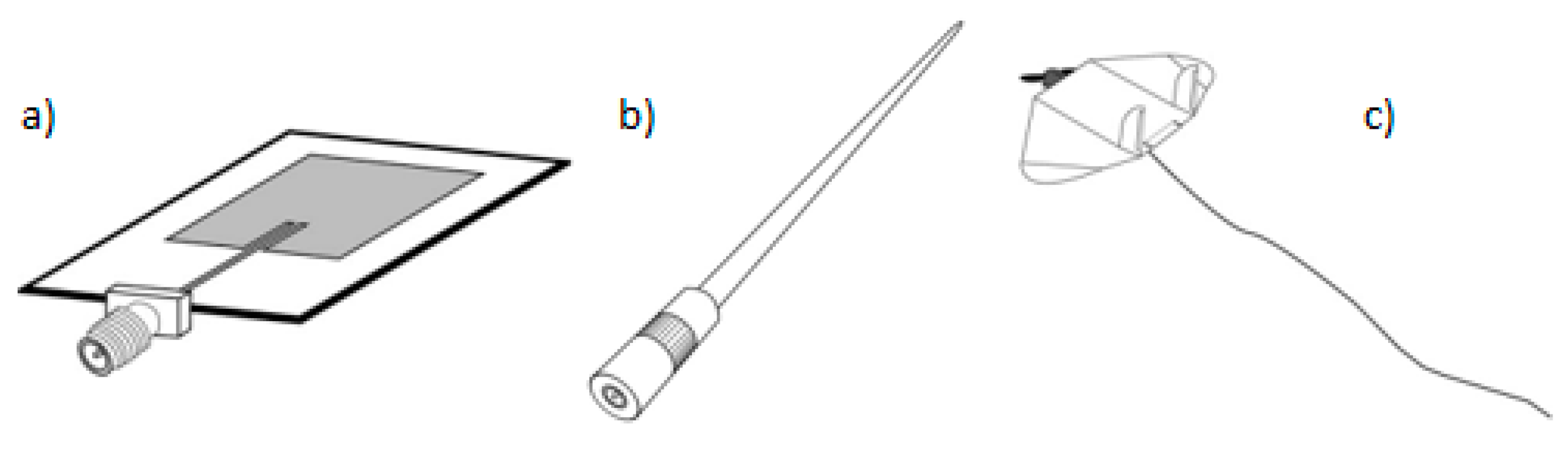
The antennas normally used for this purpose are planar antennas, whip antennas, and loose-wire antennas. Planar antennas are the most frequently used since they can be used as omnidirectional or directional antennas, which makes them very flexible. At the aerodynamic level, they do not significantly interfere with the structure.
Whip antennas, despite their low cost, have aerodynamic problems and a low gain; these are classified as omnidirectional antennas. Finally, the loose-wire antenna, which, despite its high gain allowing greater range, sees its use limited by the aerodynamic slope and risk of damage to the UAV [4].
The antenna to be studied is the planar antenna (Figure 2) because it allows for a change in the main propagation lobe of electromagnetic energy and improves the aerodynamic behavior of the aircraft, this being a crucial factor.
Planar antennas are antennas used when antenna design constraints require reduced size and weight, low cost, and high efficiency.
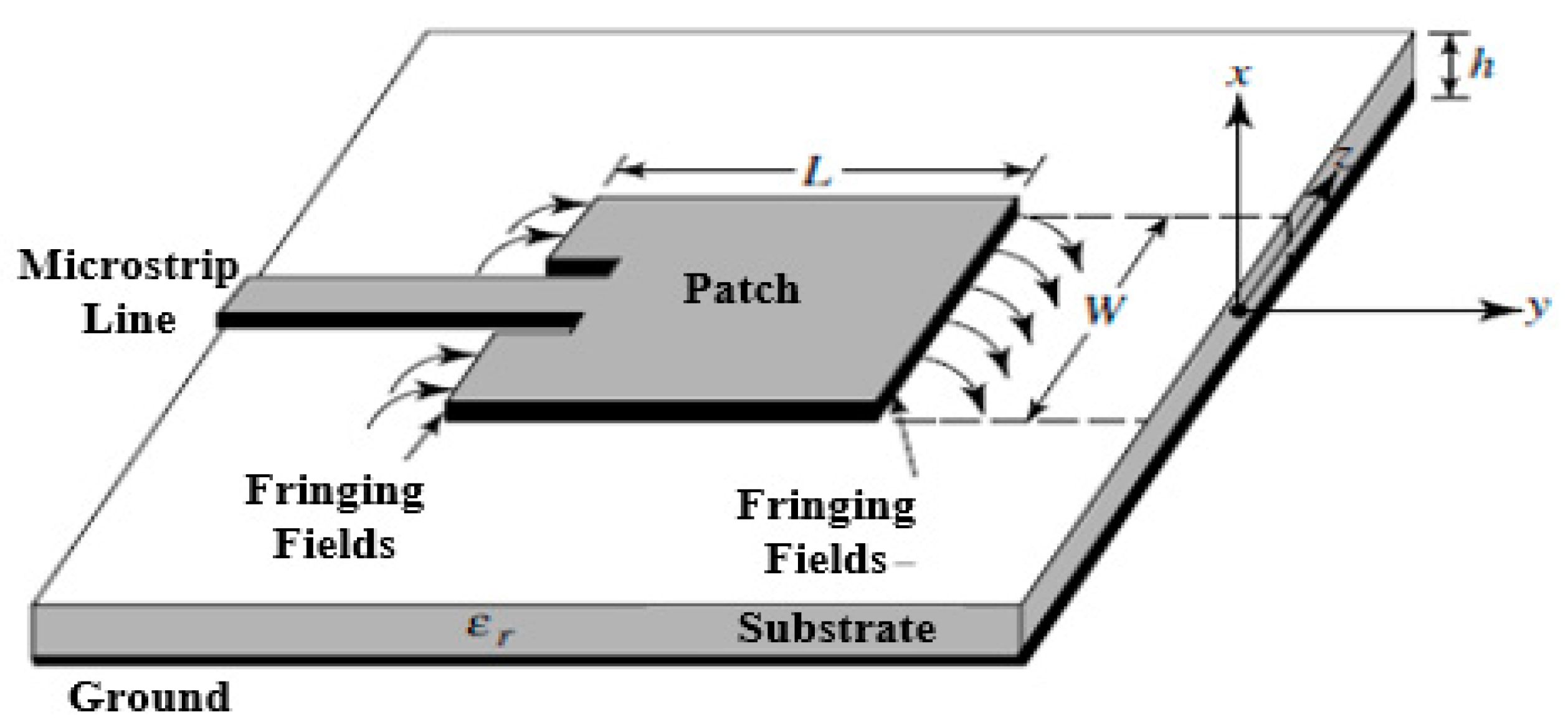
The main parameters that should be considered in this antenna project are: the relative dielectric constant of the substrate (εr); thickness h of the substrate and its size; patch configuration; and patch dimensions. These characteristics determine the radiation pattern of the antenna. Figure 3 shows a planar antenna with the above-mentioned characteristics.
The feeding method used in the antenna design was the line-feed method, given the simplicity and ease of input impedance matching.
One of several types of planar antennas are electrically steerable passive array radiator (ESPAR) antennas. These antennas allow to adapt the direction of radiation, constituted by N elements, where one element is active and the others passive elements coupled to the active. Mutual coupling is created by changing the spacing between the elements of the ESPAR antenna array and using reactance coupled with the passive elements [9].
The ESPAR antenna uses the mutual coupling to excite the parasitic elements. These elements are charged according to a variable reactance originating from varicap diodes. The variation of the value of the reactance is reflected in the alteration of the main lobe of the radiation diagram [10]. The process of changing the main lobe is called beamforming.
Unlike conventional antennas, the ESPAR antenna does not have individual lines for receiving/transmitting because only one antenna element is connected to the circuit. ESPAR antennas are an increasingly used solution because it allows beamforming, i.e., switching the main lobe, maximizing the received signal, and minimizing interference [11].
This article presents the construction of an intelligent antenna for a UAV using this technology.
3. P-ESPAR Antenna Study
In this article, we present the development of a low-cost prototype of a P-ESPAR antenna with two layers of air and one layer of FR-4. This antenna arises in the context of a previous work, where the design of an antenna with substrate RT Duroid 5870 was carried out by Marques [12].
In this sense, the configuration and simulation of the antenna is presented as well as the conclusions regarding the comparison of the results obtained through the CST Microwave Studio simulator.
The sizing of the P-ESPAR antenna took as mandatory requirements the parameters presented in Table 1.
3.1. P-ESPAR Antenna Configuration
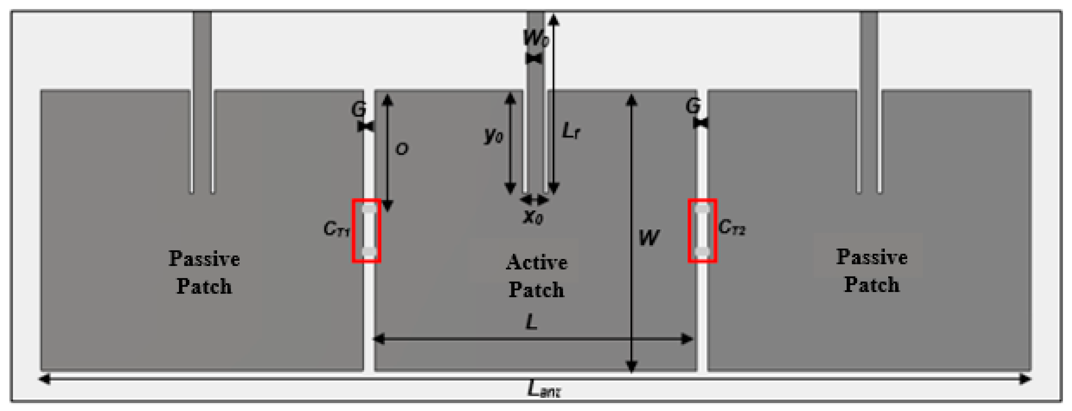
The developed P-ESPAR antenna consists of an aggregate of three elements, the middle element being the active element, and the remaining parasitic elements. The three elements have the same dimensions. The antenna has a resonance frequency of 1.33 GHz.
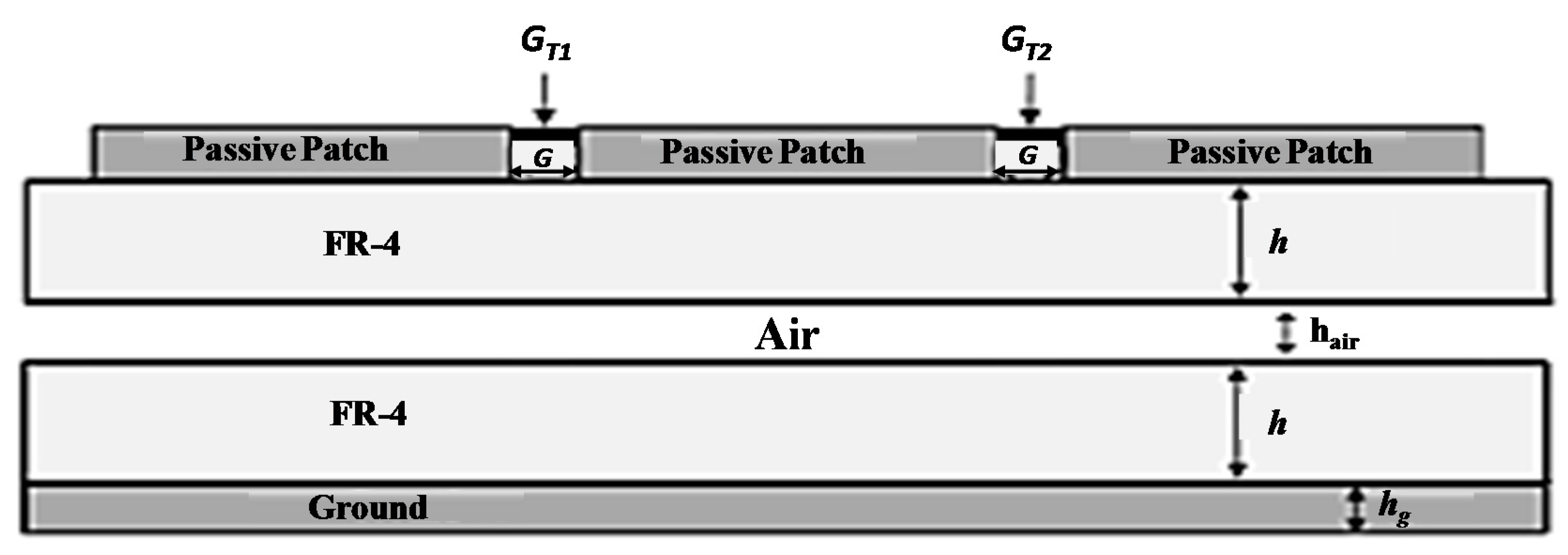
The choice of substrate was a choice conditioned by economic reasons. Initially, the chosen substrate was the RT Duroid 5870, but given its high cost, the prototype of the antenna was constructed with a substrate composed of two plates of FR-4 and an air layer of a thickness that allows to obtain a structure with the same constant (εr), its homogeneity, the tangent of the loss angle (tanδ), and the thickness (h). The equivalent model is accepted to have the same characteristics of RT DUROID 5870, but with a different thickness. For this reason, the patches were resized, the antenna simulation work repeated, and, therefore, other coupling diodes were chosen so that the antenna was perfectly adapted to the design requirements.
The antenna was constructed to present the same dielectric constant equivalent of RT Duroid 5870, for which two FR-4 substrates with one layer of air were used between them to approximate the dielectric constant to the Duroid RT 5870 values. Table 2 shows the characteristics of the FR-4 substrate and the Duroid 5870 RT for antenna sizing.
After choosing the substrate, the dimensions of the P-ESPAR antenna patch were calculated.
3.2. Equivalent Circuit
The planar antenna, from the point of view of the excitation signal source, can be described by an equivalent circuit, for example, a parallel resistor, inductor and capacitor (RLC) circuit, as shown in Figure 6.
To determine the value of R, Lc e C is necessary to carry out the study of the equivalent circuit, i.e., it is necessary to study the value of the current (), represented through:
To maximize the antenna current module, it is necessary for the imaginary component of the previous equation to be equal to zero:
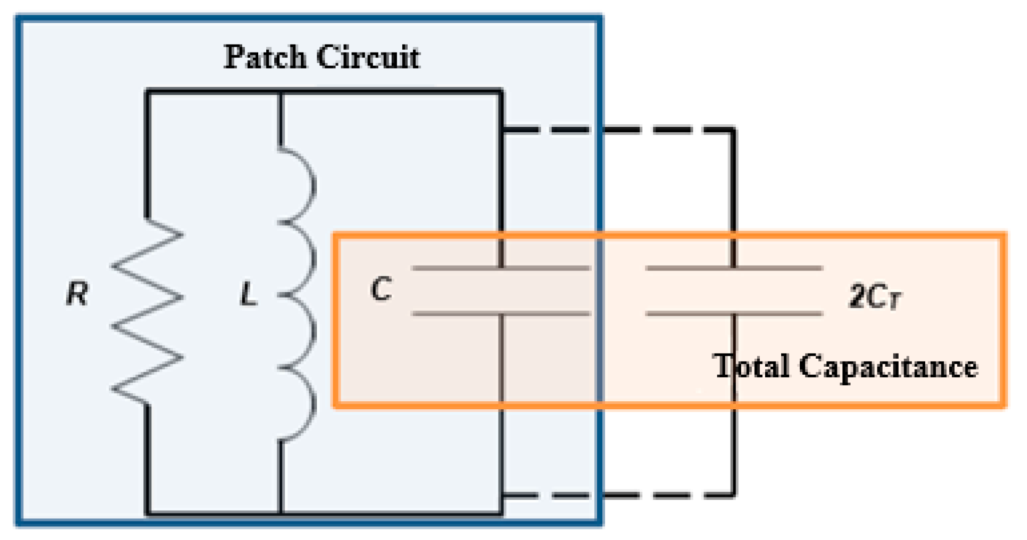
After analysis of the previous equation, it was noticed that the Lc and C were dependent on the resonant frequency of the antenna. In the case of this antenna, the variation of the radiation lobe is dependent on the capacitances of the varicap diodes. These diodes add a capacity to the 2CT, as shown in Figure 7 [16].
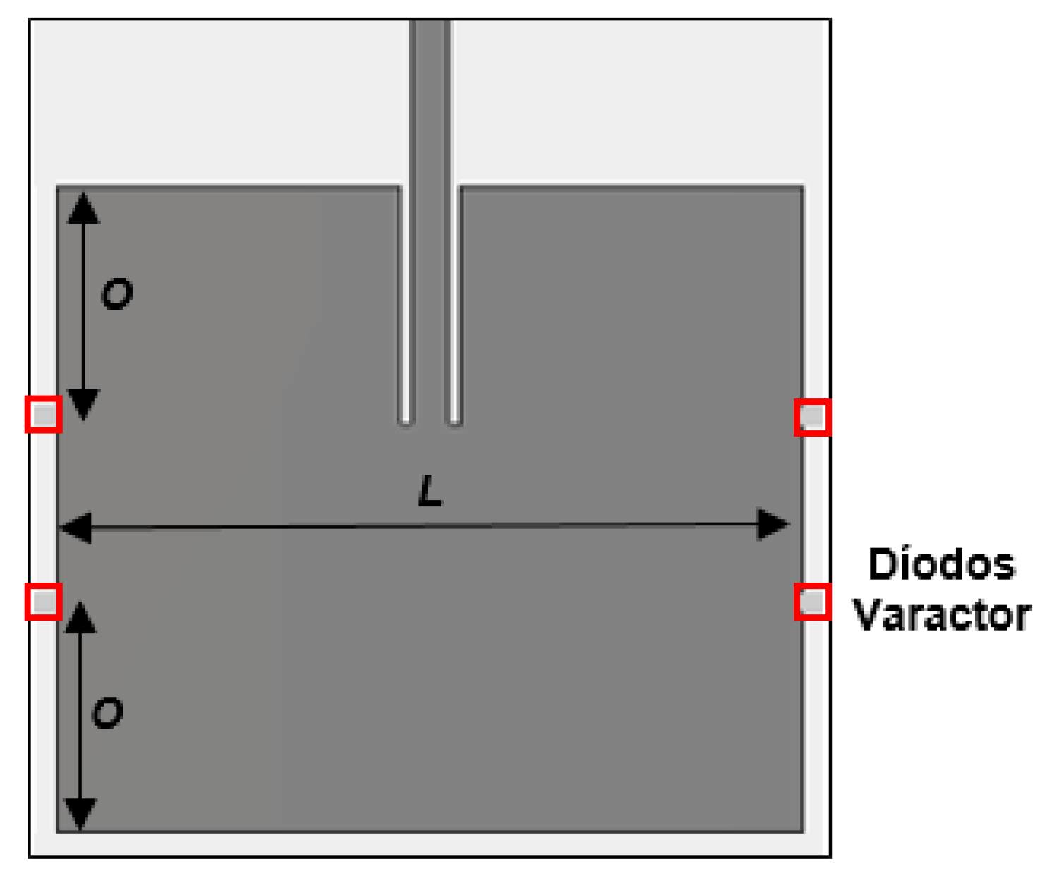
Before analysis to the system of equations, it is necessary to realize that , that is, corresponds to the value of the effective capacity of the diodes in the circuit. This value is directly dependent on the positioning of the diodes in the patch, as represented in the following equation and Figure 8, where variables O and L are represented [16]:
In case of the equivalent circuit of the antenna, with the integration of the diodes, it is necessary to change the equivalent capacity, since capacity C is added to the capacity of the diodes. The following equation represents this change:
To determine L and C, the CST Microwave studio simulator was used to obtain the resonance-frequency values of the antenna without and with diodes, f0 and fc, respectively (Table 5). The capacity of the diodes considered for simulation purposes was CT = 1 pF. The following system of equations allows Lc and C [16]:
After obtaining the results of Lc and C of the RLC circuit, it was necessary to calculate the value of resistor R. Thus, analysis was made to the circuit, considering that the relation between the complex amplitude of the current in the resistor () and the complex amplitude of the total excitation current (), where ().
Initially, it was established that reflection coefficient |S11| cannot exceed −10 dB. For this reason, the ratio in dB between the complex amplitude of the current in the resistance and the complex amplitude of the total current cannot be greater than −10 dB, as represented in the following equation. This equation is solved to obtain resistance value (Table 6):
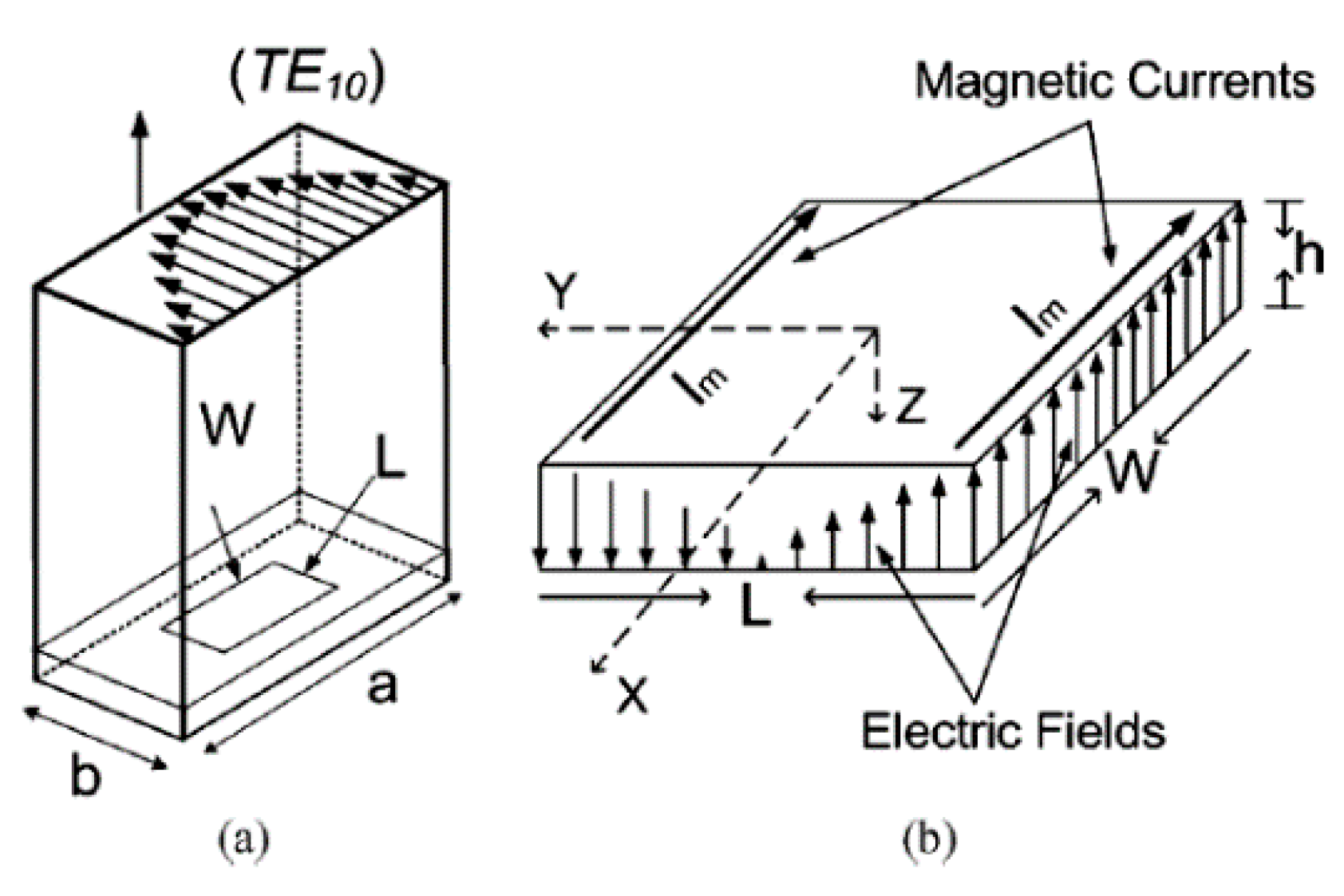
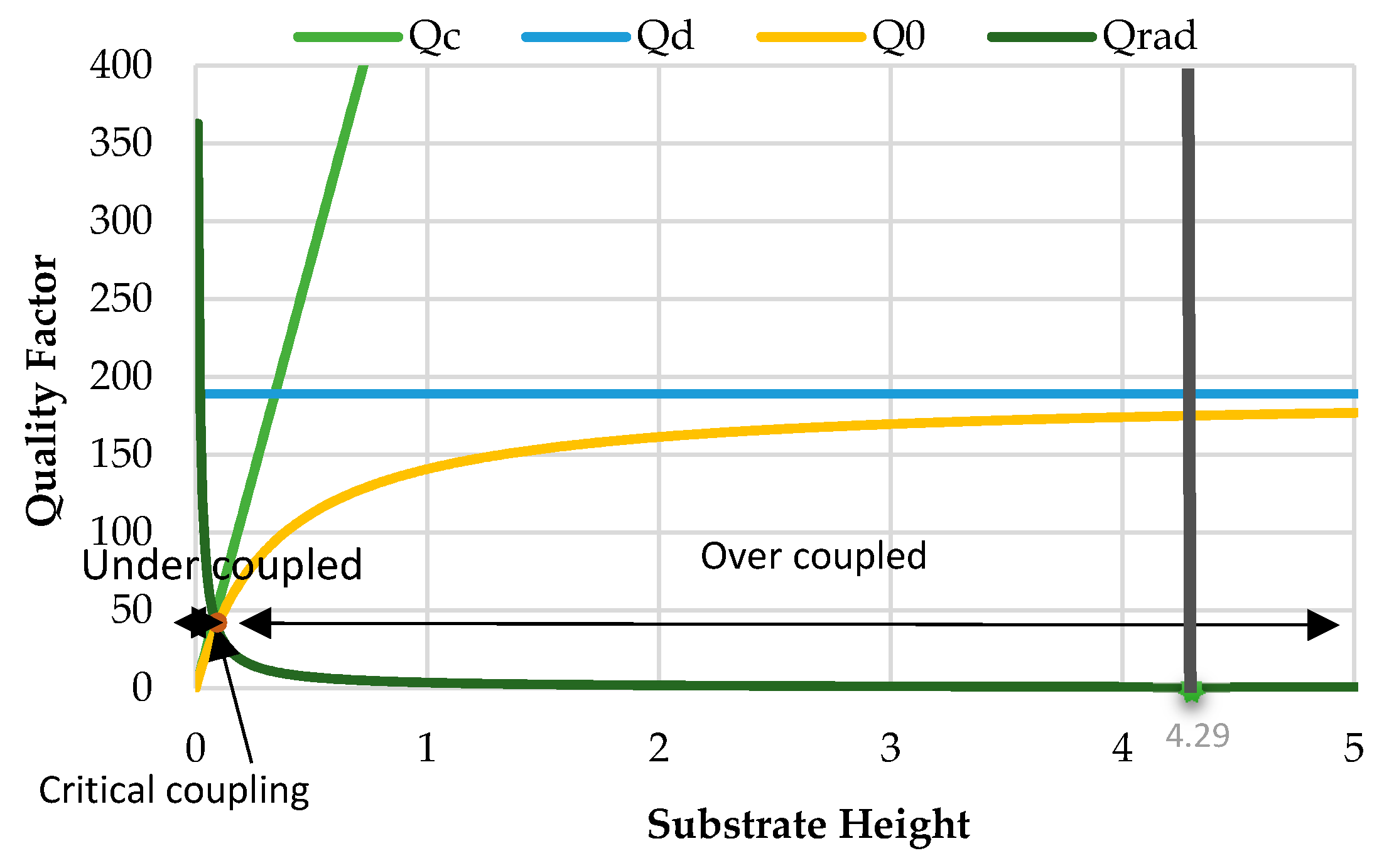
To study the coupling, it is necessary to consider the dielectric loss quality factor (Qc), antenna patch quality factor (Qd), metal loss quality factor (Qo), and the quality factor of antenna radiation (Qrad), represented by the following equations. Variables a, b, W, and L are represented in Figure 9 [17,18].
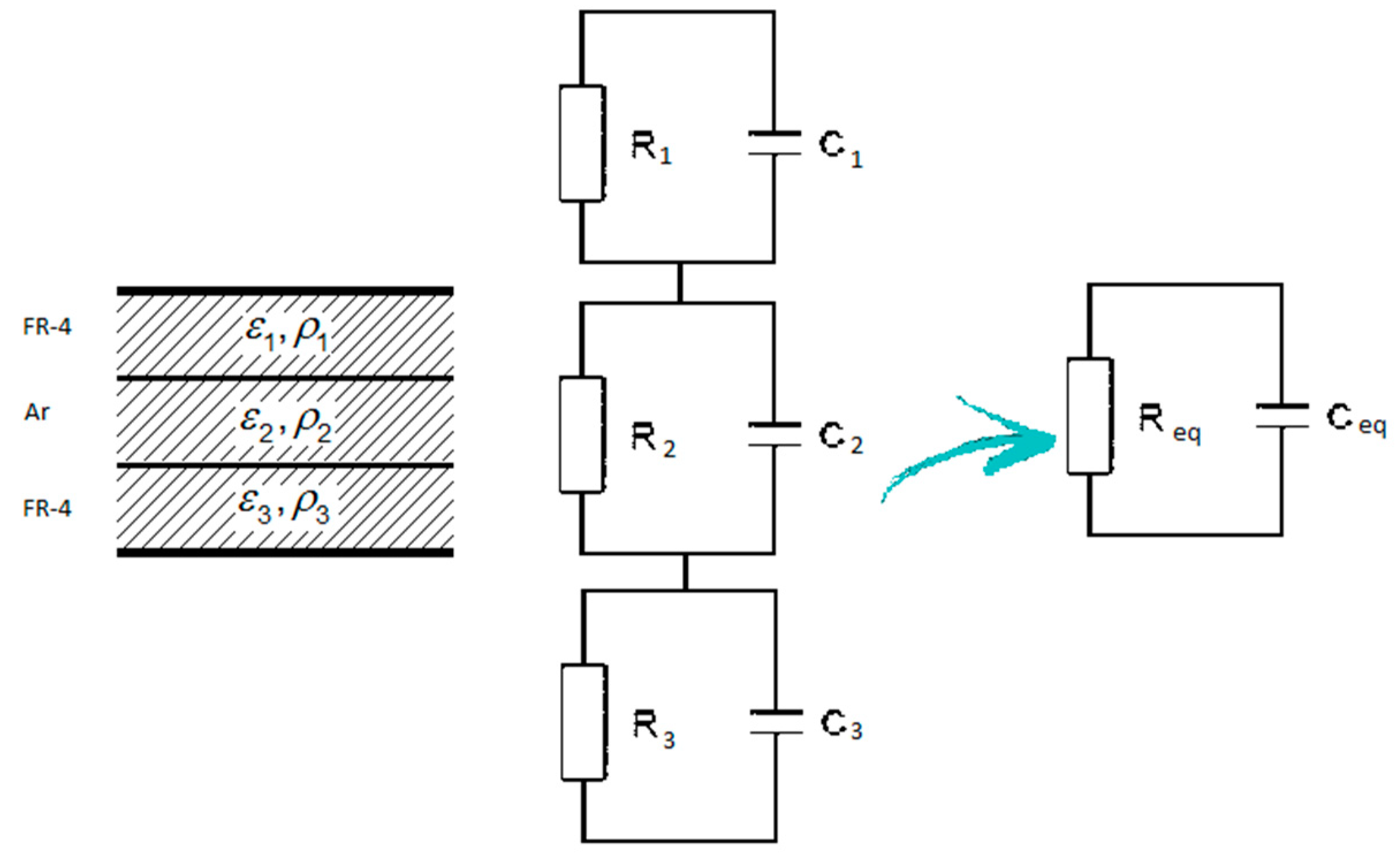
Analyzing the quality factor of the dielectric, it is perceptible that it depends on the loss tangent () of the same. In the case of the antenna with the FR-4 substrate, the medium was not homogeneous, that is, there were three media with different values of . As such, it was necessary to calculate the value of the equivalent loss tangent ().
To perform the study of the tangent of losses, it was necessary to establish the equivalent circuit for the substrate, as shown in Figure 10. Each substrate corresponded to a parallel RC circuit, whereby the three underlying substrates corresponded to the series of these circuits as represented.
For calculating , it is necessary to consider the W, L, h, and a of each substrate.
The antenna resembles a three-component system, whereby the for these circuits is given by the following equation [19,20]:
After calculating (Table 7), all conditions are met to calculate the quality factors and evaluate the antenna coupling. Thus, the coupling conditions are as follows [17]: , critical coupling; , undercoupled; and , overcoupled (Figure 11).
The used diodes were the varicap diodes of Infineon BBY53-03W. These have been selected because they were closest to the antenna capacity.
The characteristics of the varicap diodes are shown in Table 8.
After completing the entire sizing and configuration process of the P-ESPAR antenna, the simulations were performed through the CST Microwave studio software.
To obtain the different azimuths, the combinations of CT1 and CT2 diodes, shown in Table 9, were varied in the simulator (Figure 12, Figure 13, Figure 14, Figure 15 and Figure 16).
After analyzing the results of Table 9, it was possible to conclude that the imposed requirements were all fulfilled and that all the conditions for the construction and tests were gathered.
4. Control System Development
The design of the control system was performed according to the constructed antenna, i.e., in this case, the control system was scaled according to the P-ESPAR antenna with an FR-4 substrate and varicap diodes BBY53-03W.
The change in the direction of the azimuth of the radiation lobe was performed through the variation of the coupling between the elements of the aggregate, that is, through the bias voltages applied on the diodes. This way, a microcontroller and a digital potentiometer are used. The microcontroller is the means of communication between the central processor of the UAV and the digital potentiometer.
4.1. Microcontroller
The microcontroller to be integrated in the circuit has as its main function the processing of the data related to the flight of the UAV and, according to these data, send the voltage values corresponding to the communication needs to reverse bias of the diodes that ensure the value of the necessary capacities to the deflection of the antenna lobe. For the performance of this function, there are numerous microcontrollers so that, as selection factors, the following parameters were considered: user interface; support communication Serial Peripheral Interface (SPI); C programming language; USB connection; and simple and economical.
After analyzing all possibilities, the chosen microcontroller was Arduino Uno. In addition to complying with the requirements presented, it is a microcontroller that has been extensively tested and present in several simulators, which allows to test the expected result in a computational environment.
4.2. Digital Potentiometer
The digital potentiometer receives information from the microcontroller and adjusts the desired voltage at the terminals of the diodes. For this, the digital potentiometer varies the value of its resistance and, being the current constant, output voltage varies. Through the digital communication between the microcontroller and the digital potentiometer, it was possible to control the value of the resistance, which, in turn, controls the voltage value. To select the digital potentiometer, the following factors were considered: two output channels; PDIP package; SPI interface; much sensitivity in varying the resistance value; and VIN = 5 V.
After analyzing all possibilities, the selected digital potentiometer was Microship MCP42100. This potentiometer has two channels, 14 pins, 256 levels, and a resistance of 100 kΩ. It operates with voltages of 2.7–5.5 V, and the communication interface with the Arduino is SPI.
4.3. Control System Circuit
After selecting the microcontroller and the digital potentiometer, it was possible to build the control system. For this, it was necessary to define three ports of the Arduino to establish communication between the microcontroller and the digital controller. The three selected ports were Arduino digital Ports 10, 11, and 13, where Port 10 is the port responsible for the activation and deactivation of the potentiometer, Port 11 is responsible for communicating data relating to the SPI interface, and Port 13 is the port responsible for clock synchronization.
This way, Port 10 is connected to Pin 1, which is the pin responsible for activating or deactivating the digital potentiometer; Port 11 to Pin 3, which is the pin responsible for collecting data; and Port 13 to Pin 2, which is the pin responsible for clock synchronization of the digital potentiometer. The remaining pins were connected to the ground and 5 V from the Arduino as designated in the datasheet.
4.4. Control Algorithm
The P-ESPAR antenna control system was delineated by a set of criteria. These criteria were established by the needs that the communication determines according to the flight route of the UAV. In this way, the algorithm defines, by degree of priority, the variation of the wolf and finally the change of the route of the UAV.
The behavior of the P-ESPAR antenna was one of the main criteria of the algorithm. In a first phase, it was necessary to realize the capacity of the lobe to change the antenna radiation to perceive how necessary it would be to influence the route of the UAV. However, the orientation and inclination of the UAV according to the various axes are also very important factors to be considered by the algorithm of the control system.
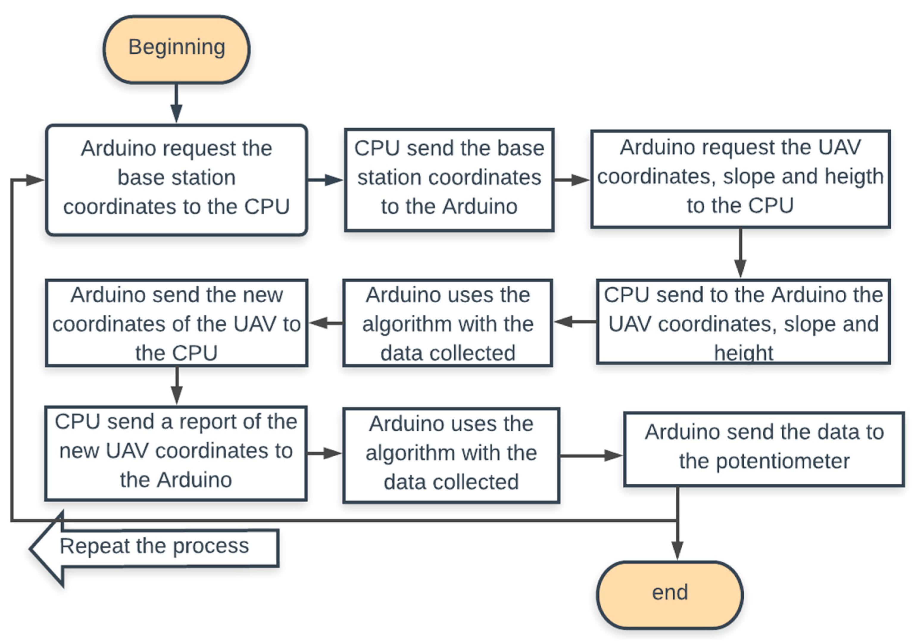
The procedures related to the algorithm mechanism are presented in the flowchart in Figure 17, with the several steps described below.
- (1)
- Control system communicates with the central processor of the UAV to request the co-ordinates of the base station;
- (2)
- after receiving the co-ordinates of the base station, the control system again communicates with the central processor of the UAV and requests the current co-ordinates, the inclination, and the height of the UAV;
- (3)
- after receiving current co-ordinates, the control-system algorithm calculates the distance between the UAV and the base station;
- (4)
- if the distance is less than or equal to 40 km, the control system selects the slope that least interferes with the route of the UAV and calculates the minimum variations required for its route;
- (5)
- the control system communicates with the central processor of the UAV, sending information about its orientation and positioning. According to the base station, the UAV must be perfectly perpendicular and parallel to the ground. It also sends information on changing the slope of the UAV;
- (6)
- after changing the route according to the communication needs, the algorithm checks the combination of capacities relative to the angle of the selected radiation lobe, and the control system communicates with the digital potentiometer to inject to the terminals of the diodes the corresponding voltages;
- (7)
- after completing the previous steps, the necessary conditions for the transmission of 10 s are fulfilled. At the end of the transmission, we return to Step (2).
5. Construction and Implementation of the Smart Antenna
5.1. Smart Antenna Construction
The implementation of the communication system was carried out in two phases: antenna construction, and the construction of the control system.
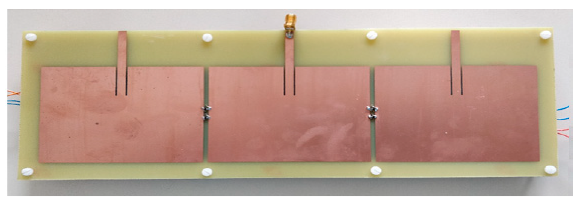
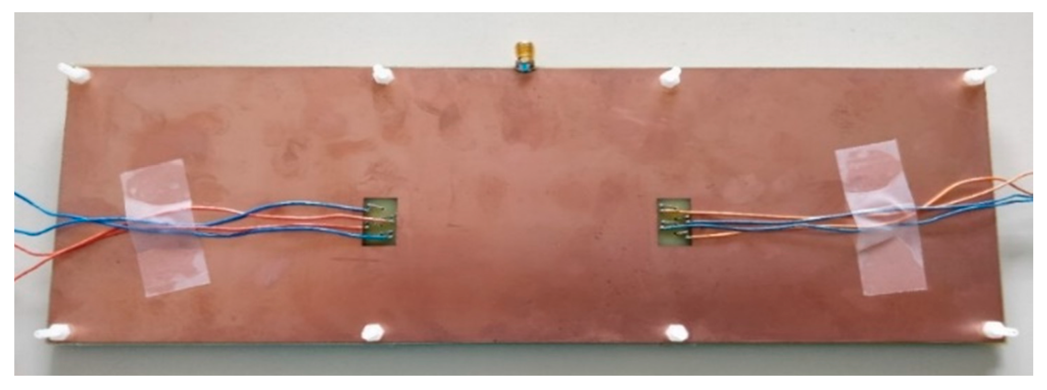
The P-ESPAR antenna was built in the laboratories of the Instituto Superior Técnico. In Figure 18, the top of the antenna is shown and, in Figure 19, its bottom part.
The circuit was printed in the IST at Taguspark. The circuit uses three cable terminal board ports with three outputs that are used as terminals of the digital potentiometer.
5.2. Experimental Results
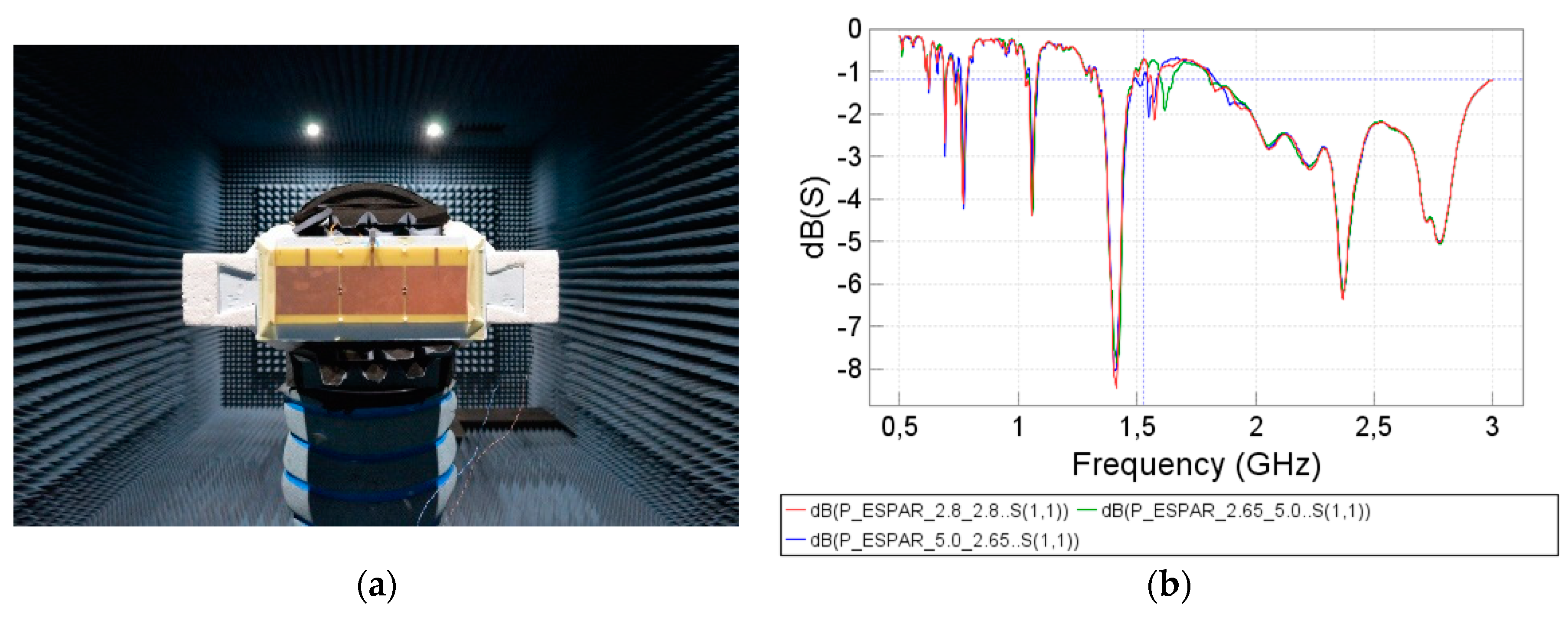
The experimental results of the antenna were obtained in the anechoic chamber of the scientific area of the Institute of Telecommunications at IST because technical limitations were the only available conditions to measure the S11 (reflection coefficient of the antenna) and the radiation diagram of the antenna (Figure 20, Figure 21, Figure 22, Figure 23 and Figure 24).
The combinations of the used diodes can be seen in Table 10.
Starting with the analysis of the |S11| parameter, it was possible to verify that the resonance frequency was very close to the frequency in which antenna design was carried out, that is, the measured value was 1.41 GHz, and the antenna was dimensioned for 1.33 GHz. To correct this small deviation, it would be necessary to study the behavior of the resonance frequency with slight changes of distances 0 in the patch.
Regarding the tax requirement of |S11| ≤ −10 dB, this was not observed in the results obtained through the network analyzer. In the results obtained through the simulator, the requirement was always fulfilled by a comfortable margin, so it would be necessary to correct the height of the hg air layer and to verify, through the network analyzer, the variations of the parameter |S11|. The height of the air layer was not constant throughout the antenna since it is impossible to obtain the accuracy imposed by the simulation.
In addition to the hg correction, there was still interference caused by power cables with a length approximately equal to λ/2. During the scanning from 0 to 2 GHz, it was possible to observe the interference caused by the cables.
Analyzing the radiation diagram, it was possible to verify that the radiation lobe of the P-ESPAR antenna was displaced −6° in relation to the expected azimuth. This variation corresponds to the side on which the power cables were placed, so they could be responsible for this small deviation.
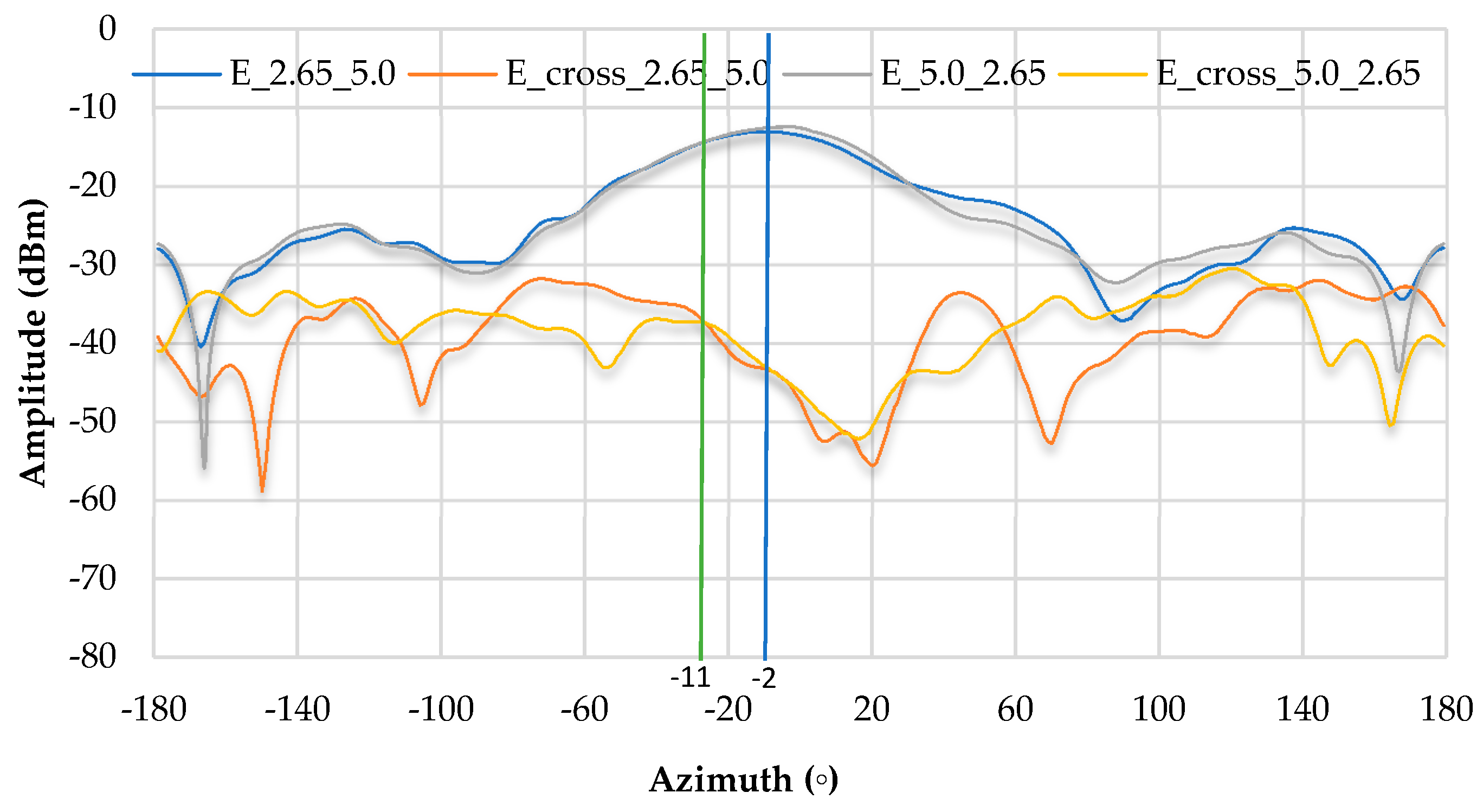
In relation to the azimuthal variation of ±5° with 0° azimuth, extremely positive results were obtained.
Inspecting the results, it was possible to verify that the variation range of the main lobe was between −11° and −2°.
These results summarized in Table 11 prove that the measured results go against the simulated ones, this being because there are integrated elements in the antenna that the simulator does not allow to consider. However, it is possible to improve the obtained results with minor changes to the insulation of the feed paths of the P-ESPAR antenna diodes and by reducing the length of the cables of the diode feed system.
6. Conclusions
The Portuguese Air Force (FAP) is the branch of Army Forces with the most knowledge on UAVs in Portugal. The algorithm integrated in the Arduino was based on the orientation methodology used in UAVs by the FAP. The developed algorithm also uses procedures to change the UAV route, taking into account the limit conditions given by experienced officers in these aircraft. The implemented solution changes the route of the UAV for 10 s, whenever line-of-sight communication is not possible, i.e., the control system, in this case controlled by an Arduino, changes the flight path of the UAV, if necessary, during the time of the communication.
After completing and validating the algorithm of the control system, the P-ESPAR antenna and the electronic circuit were built to integrate the control system.
P-ESPAR antenna tests were performed in the anechoic chamber of the Telecommunications Institute at IST. Through the analysis presented in a previous section, it was possible to conclude that the results were not the same as those in the simulator, but rather close. These tests allow to verify the possibility for variation of the radiation lobe, as well as adaptation for the dimensioned frequency. It was also possible to conclude which factors were detrimental to the measurements, and how to provide the necessary changes.
As previously mentioned, the construction of the antenna with two substrates of FR-4 and an air layer was an economical option that allowed the dimensioning and development of a prototype. The built antenna is not a final version, but an intermediate step, to demonstrate the potential of this solution to the FAP.
Author Contributions
Conceptualization, A.B.; data curation, A.F.A.C.; investigation, J.P.N.T. and M.J.M.M.
Funding
This work was supported by FCT through IT, under the project UID/EEA/50008/2013.
Acknowledgments
We thank Carlos Brito and João Pina who accompanied the entire construction process of the antenna.
Conflicts of Interest
The authors declare no conflict of interest.
References
- Rodrigues, F.D.S. O Poder Aéreo na transformação da defesa. Cadernos do IDN 2009, 4, 3–10. (In Portuguese) [Google Scholar]
- Ruano, E.M.B.; Baptista, A.; Martins, M.J.; Torres, J.P.N.T. Comparative analysis of two antennas for communication in 2.4 GHz. Far East J. Electron. Commun. 2018, 13, 457–476. [Google Scholar] [CrossRef]
- Winnefeld, J.A.; Kendall, F. Unmanned systems integrated roadmap FY 2011-2036. Available online: https://fas.org/irp/program/collect/usroadmap2011.pdf (accessed on 6 December 2018).
- Valavanis, K.P.; Vachtsevanos, G.J. Handbook of Unmanned Aerial Vehicles; Springer: Berlin/Heidelberg, Germany, 2015; pp. 1386–1438. [Google Scholar]
- De Sousa, M.Q.M.N. Uso de Veículos Aéreos Não Tripulados no Sistema Tático de Guerra Eletrônica (SITAGE). Available online: http://www.ccomgex.eb.mil.br/cige/sent_colina/7_edicao_agosto_08/Artigos%20Revista%20Edicao%207/JA%20FEITO/Artigo_Maj%20Nogueira_uav_corrigido3.pdf (accessed on 6 December 2018). (In Portuguese).
- Costa, A.G.D. Sistema de Rádio Comunicações para UAV. Master’s Thesis, Universidade de Aveiro, Aveiro, Portugal, 2015. Available online: https://ria.ua.pt/bitstream/10773/15968/1/Sistemas%20de%20r%C3%A1dio%20comunica%C3%A7%C3%B5es%20para%20UAV.pdf (accessed on 6 December 2018). (In Portuguese).
- Antena Omni VS. Antena Direcional. Available online: https://docplayer.com.br/15656699-Antena-omni-vs-antena-direcional.html (accessed on 6 December 2018). (In Portuguese).
- Garg, R.; Bhartia, P.; Bahl, I.J.; Ittipiboon, A. Microstrip Antenna Design Handbook, 1st ed.; Artech House: Norwood, MA, USA, 2001; pp. 1–40. [Google Scholar]
- Abdalrazik, A.; Soliman, H.; Abdelkader, M.F.; Abuelfadl, T.M. Power performance enhancement of underlay spectrum sharing using microstrip patch espar antenna. In Proceedings of the Wireless Communications and Networking Conference (WCNC), Doha, Qatar, 3–6 April 2016; pp. 1–6. [Google Scholar]
- Nikkhah, M.R.; Loghmannia, P.; Rashed-Mohassel, J.; Kishk, A.A. Theory of ESPAR design with their implementation in large arrays. IEEE Trans. Antennas Propag. 2014, 62, 3359–3364. [Google Scholar] [CrossRef]
- Balanis, C. Antenna Theory Analysis and Design; John Wiley and Sons: Hoboken, NY, USA, 2005. [Google Scholar]
- Marques, P.; Martins, M.; Baptista, A.; Torres, J.P.N. Communication Antenas for UAVs. J. Eng. Sci. Tech. Rev. 2018, 11, 90–102. [Google Scholar] [CrossRef]
- FR4 Data Sheet. Available online: https://www.farnell.com/datasheets/1644697.pdf (accessed on 11 December 2016).
- RT/duroid ® 5870/5880. Rogers Corporation. 2016. Available online: https://www.rogerscorp.com/documents/606/acm/RT-duroid-5870-5880-Data-Sheet.pdf (accessed on 11 December 2016).
- Marques, P. Antenas de Comunicação para UAVs Instituto Superior Técnico, Lisboa, Portugal. 2016. Available online: https://fenix.tecnico.ulisboa.pt/downloadFile/1407770020545454/1.%20Dissertacao%20de%20Mestrado%20Antenas%20Comunicacoes%20para%20UAVs.pdf (accessed on 6 December 2018). (In Portuguese).
- Luther, J. Microstrip Patch Electrically Steerable Parasitic Array Radiators. Ph.D. Thesis, University of Central Florida, Orlando, FL, USA, 2013; pp. 10–51. [Google Scholar]
- Karnati, K.K.; Yusuf, Y.; Ebadi, S.; Gong, X. Theoretical analysis on reflection properties of reflectarray unit cells using quality factors. IEEE Trans. Antennas Propag. 2013, 61, 201–210. [Google Scholar] [CrossRef]
- Bozzi, M.; Germani, S.; Perregrini, L. A figure of merit for losses in printed reflectarray elements. IEEE Antennas Wirel. Propag. Lett. 2004, 3, 257–260. [Google Scholar] [CrossRef]
- Hayt, W.H.; Buck, J.A. Engineering Eletromagnetics, 8th ed.; McGraw-Hill Education: New York, NY, USA, 2010; pp. 109–173. [Google Scholar]
- Loftness, R.L. The Dielectric Losses of Various Filled Phenolic Resins. Ph.D. Thesis, The Swiss Federal Institute Of Technology Zurich, Zurich, Switzerland, 1952. [Google Scholar]
Figure 1.
Unmanned vehicle (UV) classification by field of performance.


Figure 3.
Specification of a planar antenna [8].
Figure 3.
Specification of a planar antenna [8].

Figure 4.
Structure and dimensions of the P-ESPAR antenna in the frontal perspective [15].
Figure 4.
Structure and dimensions of the P-ESPAR antenna in the frontal perspective [15].

Figure 5.
Corss-section view of the P-ESPAR antenna.

Figure 6.
Equivalent circuit of planar antenna [16].
Figure 6.
Equivalent circuit of planar antenna [16].

Figure 7.
Equivalent circuit of P-ESPAR antenna [16].
Figure 7.
Equivalent circuit of P-ESPAR antenna [16].

Figure 8.
Representation of variables O and L in the patch.

Figure 9.
Variation of the magnetic field in the substrate for the fundamental mode [17].
Figure 9.
Variation of the magnetic field in the substrate for the fundamental mode [17].

Figure 10.
Representation of the equivalent circuit of antenna substrates with FR-4 [18].
Figure 10.
Representation of the equivalent circuit of antenna substrates with FR-4 [18].

Figure 11.
Quality factor as a function of substrate height.

Figure 12.
Results obtained with FR-4 to −10°.

Figure 13.
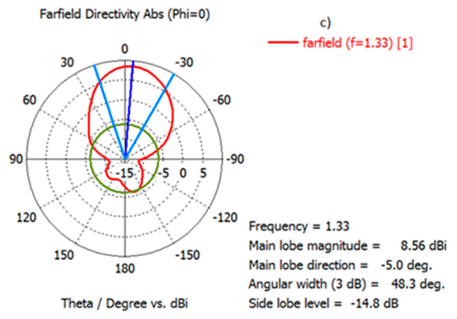
Results obtained with FR-4 for −5°.

Figure 14.
Results obtained with FR-4 for 0°.

Figure 15.
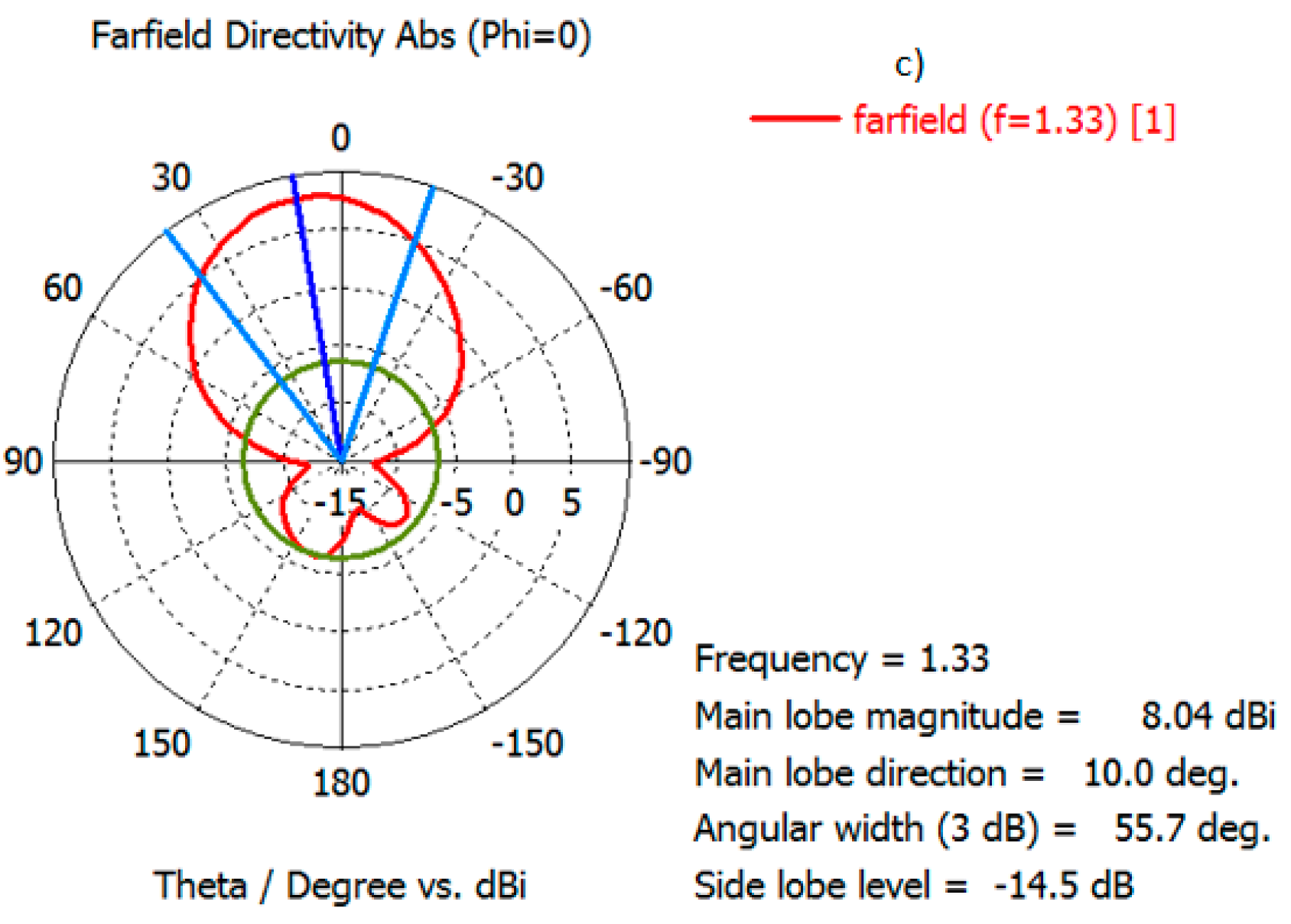
Results obtained with FR-4 for 5°.

Figure 16.
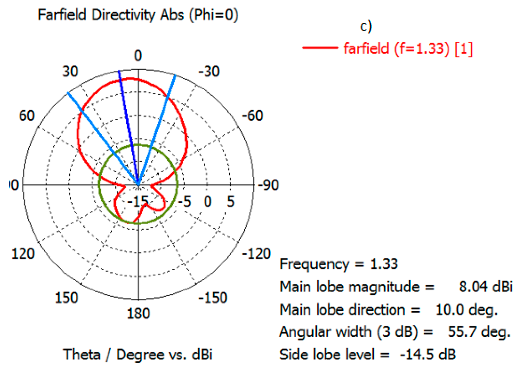
Results obtained with FR-4 to −10°.

Figure 17.
Flowchart of the process.

Figure 18.
Top view of the P-ESPAR antenna.

Figure 19.
Bottom view of the P-ESPAR antenna.

Figure 20.
(a) Antenna in the anechoic chamber and (b) respective results of |S11| with a variation of 0 ± 5°.
Figure 20.
(a) Antenna in the anechoic chamber and (b) respective results of |S11| with a variation of 0 ± 5°.

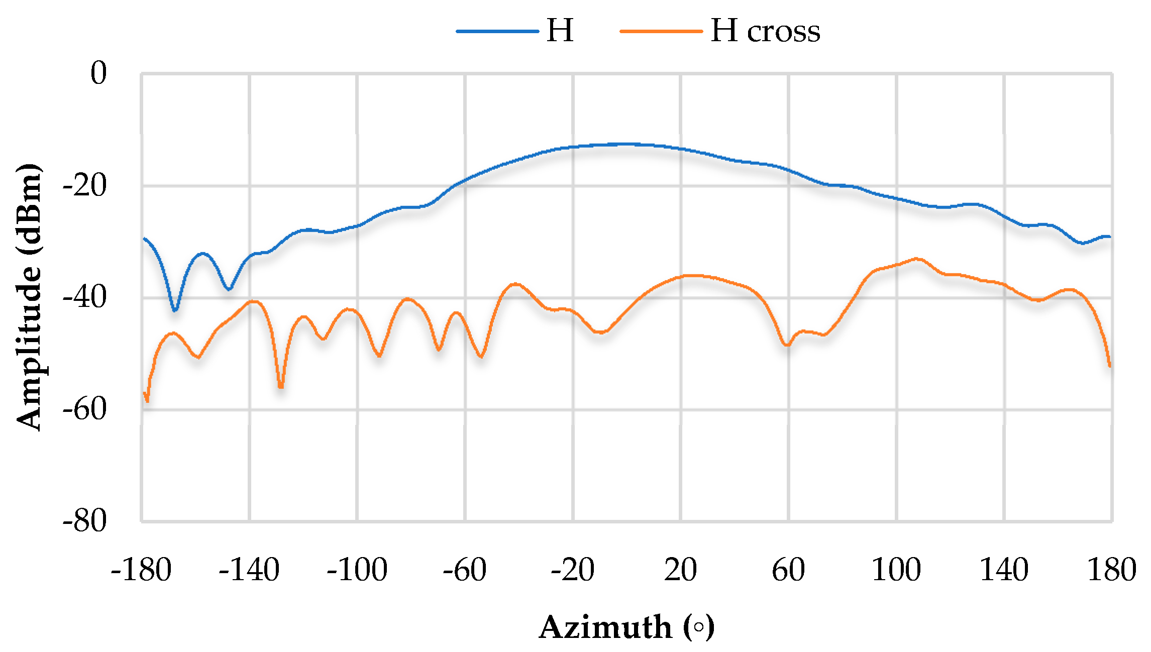
Figure 21.
Representation of the radiation diagram for 0° in the H plane.

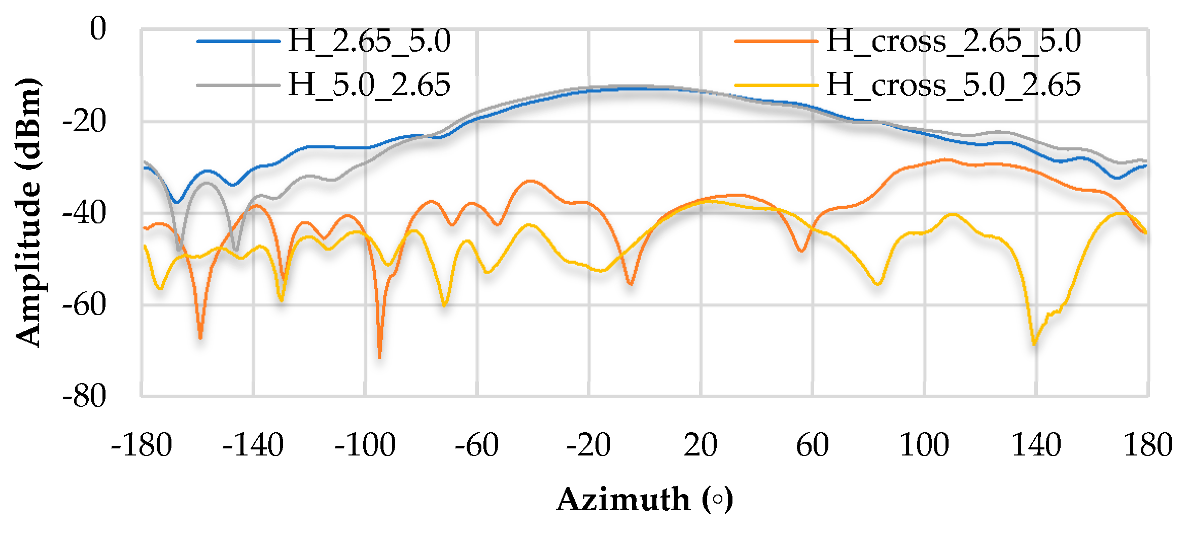
Figure 22.
Comparison of the radiation diagram to ± 5° in the H plane.

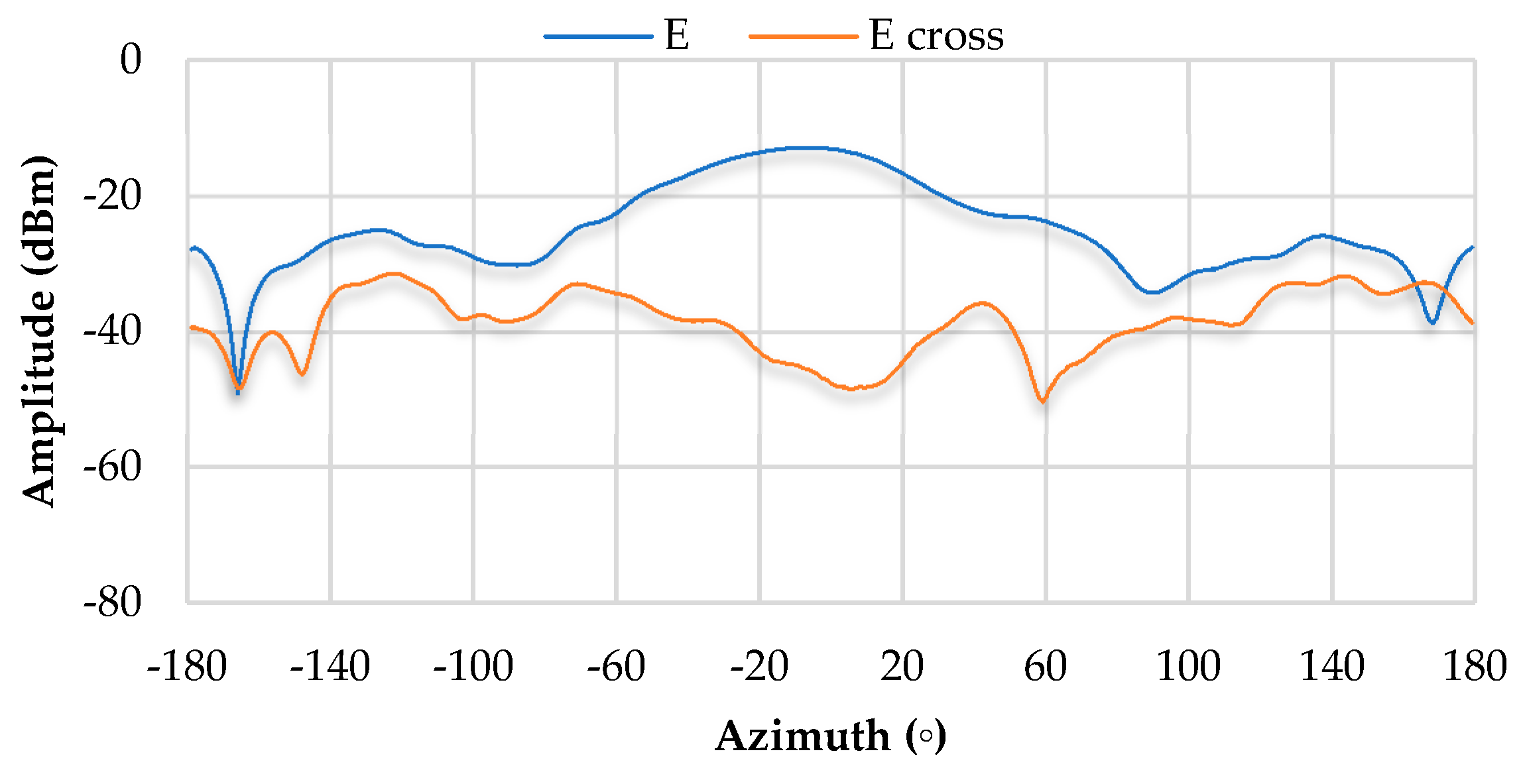
Figure 23.
Representation of the radiation diagram for 0° in the E plane.

Figure 24.
Comparison of the radiation diagram to ± 5° in the E plane.


Table 1.
Requirements for the planar electrically steerable passive array radiator (P-ESPAR) antenna design.
Table 1.
Requirements for the planar electrically steerable passive array radiator (P-ESPAR) antenna design.
| Frequency | 1.330 GHz |
| Gain | >3 dB |
| Bandwidth | >8 MHz |
| Coefficient of reflection |S11| | ≤−10 dB |
| FR-4 | RT Duroid 5870 | ||
|---|---|---|---|
| r | 4.700 | r | 2.330 ± 0.020 |
| tanδ | 0.014 | tanδ | 5.000 × 10⁻⁵ |
| Thickness | 1.575 mm | Thickness | 1.575 mm |
Table 3.
Dimensions of the antenna with two substrate FR-4 plates and one layer of air.
| FR-4 | |||
|---|---|---|---|
| Dimension | Optimization | ||
| Patch width | W | 87.400 mm | 84.300 mm |
| Patch length | Lp | 71.760 mm | 65.600 mm |
| Antenna length | Lant | 274.900 mm | 274.900 mm |
| Transmission line width | W0 | 3.500 mm | 4.500 mm |
| Substrate thickness | H | 1.575 mm | 1.575 mm |
| Ground thickness | hg | 0.019 mm | 0.019 mm |
| Air layer thickness | har | 1.090 mm | 1.090 mm |
| Total thickness | htotal | 4.240 mm | 4.240 mm |
| Diode length | Gd | 3.000 mm | 3.000 mm |
| Position of mutual coupling of the diode | O | 30.000 mm | 30.000 mm |
| Insert feed point location | y0 | 22.842 mm | 20.000 mm |
| Resonance resistance | Rin(y = 0) | 105.403 Ω | 105.403 Ω |
| Input resistance for insert feed | Rin(y = y0) | 50.000 Ω | 50.000 Ω |
Table 4.
Frequency of resonance.
| Two Layers of FR-4 with One Layer of Air | |
|---|---|
| 1.368 GHz | |
| 1.330 GHz |
Table 5.
Results obtained for the calculation of L and C.
| Two Layers of FR-4 with One Layer of Air | |
|---|---|
| f0 [GHz] | 1.388 |
| fc [GHz] | 1.383 |
| O [mm] | 31.000 |
| [pF] | 0.065 |
| Lc [nH] | 2.668 |
| C [pF] | 4.932 |
Table 6.
Values obtained from the RLC equivalent circuit.
| Two Layers of FR-4 with One Layer of Air | |
|---|---|
| R [kΩ] | 2.978 |
| Lc [nH] | 2.668 |
| C [pF] | 4.932 |
Table 7.
Parameters and results.
| 0.014 | 274.900 mm | ||
| 0.000 | 1.575 mm | ||
| 0.014 | 1.090 mm | ||
| 4.700 | 0.725 nF | ||
| 1.00059 | 0.220 nF | ||
| 99.820 mm | 0.00528755 |
Table 8.
Characteristics of varicap diodes.
| BBY53-03W | |||
|---|---|---|---|
| Values | |||
| Minimum | Typical | Maximum | |
| Variable capacity (CT) 1 | |||
| VR = 1V | 4.8 pF | 5.3 pF | 5.8 pF |
| VR = 3V | 1.85 pF | 2.4 pF | 3.1 pF |
| Diode Inductance (LS) | - | 1.8 nH | - |
| Diode resistance (RS) VR = 1V | - | 0.47 Ω | - |
Table 9.
Results of the P-ESPAR antenna simulation with FR-4 using varicap diodes BBY53-03W.
| Direction of Wolf Main [°] | P-ESPAR Antenna Characteristics | ||||||
|---|---|---|---|---|---|---|---|
| G (dBi) | HPBW (˚) | fc (GHz) | |S11| (dB) | BW (MHz) | CT1 (pF) | CT2 (pF) | |
| −10 | 8.09 | 55.5 | 1.3625 | −15.37 | 15.9 | 1.1 | 3.1 |
| −5 | 8.56 | 48.3 | 1.3775 | −15.09 | 23.4 | 1.5 | 2.7 |
| 0 | 8.11 | 59.4 | 1.3750 | −15.95 | 23.4 | 2.6 | 2.6 |
| 5 | 8.55 | 48.2 | 1.3800 | −15.44 | 23.2 | 2.7 | 1.5 |
| 10 | 8.04 | 55.7 | 1.3650 | −15.37 | 16.6 | 3.1 | 1.1 |
Table 10.
CT combinations for different angular variations.
| CT1 | CT2 | |||
|---|---|---|---|---|
| [pF] | [V] | [pF] | [V] | |
| −5° | 2.70 | 2.65 | 2.00 | 5.00 |
| 0° | 2.6 | 2.80 | 2.6 | 2.80 |
| 5° | 2.00 | 5.00 | 2.70 | 2.65 |
Table 11.
Conclusions drawn from the tests carried out in the anechoic chamber.
| Plane E | Plane H | |S11| | Polarization | frc | |||
|---|---|---|---|---|---|---|---|
| CT1 | CT2 | Maximum Direction | Maximum Direction | HPBW | |||
| 1.9 pF | 2.7 pF | −11° | 0° | 360° | −8.0 dB | Linear Vertical | 1.41 GHz |
| 2.6 pF | 2.6 pF | −6° | 0° | 360° | −8.3 dB | ||
| 2.7 pF | 1.9 pF | −2° | 0° | 360° | −8.0 dB | ||
© 2018 by the authors. Licensee MDPI, Basel, Switzerland. This article is an open access article distributed under the terms and conditions of the Creative Commons Attribution (CC BY) license (http://creativecommons.org/licenses/by/4.0/).
Share and Cite
MDPI and ACS Style
Carneiro, A.F.A.; Torres, J.P.N.; Baptista, A.; Martins, M.J.M. Smart Antenna for Application in UAVs. Information 2018, 9, 328. https://doi.org/10.3390/info9120328
AMA Style
Carneiro AFA, Torres JPN, Baptista A, Martins MJM. Smart Antenna for Application in UAVs. Information. 2018; 9(12):328. https://doi.org/10.3390/info9120328
Chicago/Turabian StyleCarneiro, António Fernando Alves, João Paulo N. Torres, António Baptista, and Maria João M. Martins. 2018. "Smart Antenna for Application in UAVs" Information 9, no. 12: 328. https://doi.org/10.3390/info9120328
Note that from the first issue of 2016, this journal uses article numbers instead of page numbers. See further details here.