SeMiner: A Flexible Sequence Miner Method to Forecast Solar Time Series
by
 ,
,
Sérgio Luisir Díscola Junior
1,2,*,†,‡ ,
,
José Roberto Cecatto
3,‡,
Márcio Merino Fernandes
1,‡ and
Marcela Xavier Ribeiro
1,‡ 1
Department of Computer Science, Federal University of São Carlos (UFSCar) , São Carlos 13565-905, Brazil
2
Federal Institute of Education, Science and Technology of São Paulo (IFSP), São Carlos 13565-905, Brazil
3
National Institute for Space Research (INPE), São José dos Campos 12227-010, Brazil
*
Author to whom correspondence should be addressed.
†
Current address: Federal University of São Carlos, Rodovia Washington Luis, km 235, São Carlos 13565-905, Brazil
‡
These authors contributed equally to this work.
Information 2018, 9(1), 8; https://doi.org/10.3390/info9010008
Submission received: 12 December 2017
/
Revised: 29 December 2017
/
Accepted: 2 January 2018
/
Published: 4 January 2018
(This article belongs to the Special Issue Information Technology: New Generations (ITNG 2017))
Abstract
:X-rays emitted by the Sun can damage electronic devices of spaceships, satellites, positioning systems and electricity distribution grids. Thus, the forecasting of solar X-rays is needed to warn organizations and mitigate undesirable effects. Traditional mining classification methods categorize observations into labels, and we aim to extend this approach to predict future X-ray levels. Therefore, we developed the “SeMiner” method, which allows the prediction of future events. “SeMiner” processes X-rays into sequences employing a new algorithm called “Series-to-Sequence” (SS). It employs a sliding window approach configured by a specialist. Then, the sequences are submitted to a classifier to generate a model that predicts X-ray levels. An optimized version of “SS” was also developed using parallelization techniques and Graphical Processing Units, in order to speed up the entire forecasting process. The obtained results indicate that “SeMiner” is well-suited to predict solar X-rays and solar flares within the defined time range. It reached more than 90% of accuracy for a 2-day forecast, and more than 80% of True Positive (TPR) and True Negative (TNR) rates predicting X-ray levels. It also reached an accuracy of 72.7%, with a TPR of 70.9% and TNR of 79.7% when predicting solar flares. Moreover, the optimized version of “SS” proved to be 4.36 faster than its initial version.
1. Introduction
Solar Flares are sudden releases of large amounts of energy (– erg) from the active regions of the solar atmosphere. These phenomena can last from tens of seconds up to a few hours, depending on the intensity, emitting a broad spectrum of electromagnetic radio waves radio, such as X-rays or even gamma-rays. The X-ray flux measured within the band 1–8 Angstrom of the solar spectrum is used to classify solar flares into four ranges, which can be recorded by artificial satellite sensors. Considering an increasing order of X-ray emitted by the Sun, solar flares are classified as “B” (the weakest), followed by those classified as “C”, “M”, and “X” (the strongest).
Solar Flares impact High Frequency (HF) and Very High Frequency (VHF) radio communications because of the X-ray influence on HF/VHF paths inside the ionosphere [1,2]. Solar flares and their high X-rays emissions can also impact the Global Positioning System (GPS), and electricity power grids, possibly causing blackouts. Consequently, because of those and other effects from X-ray fluxes on Earth, it is imperative to develop and enhance forecasting methods.
There are two kinds of events related to solar flares: (1) the solar flares themselves; and (2) the increase of the X-ray background level. Solar Flares occur when there is a sudden variation on the level of X-ray emissions. On the other hand, a smooth increase in those emissions characterizes an “increase in the X-ray background level”. Forecasting both events is essential because they may cause those impacts aforementioned. Solar flares can be more damaging than the increase of X-ray background level. However, an increase in background level can be an indication of an imminent occurrence of a more significant solar event.
Recently, researchers have been increasing efforts to forecast solar flares using data mining techniques. Although necessary, works focussing on background level forecasting are relatively rare. The core of these methods resides in the preparation of raw data (also known as the pre-processing step) that are submitted to the classifiers. The forecasting methods follow the usual steps of a data mining process: acquisition and pre-processing of data, feature selection, classification, validation, and testing. They differ according to the solar parameters used, the preparation of both, training and testing datasets, and the adopted pre-processing and classification methods. They also differ on what is foreseen: one option is to forecast solar flares grouped under a set of categories, another produces a specific forecast for each class of solar flares.
The classifiers used by forecasting methods were developed aiming to classify tuples with a given label, describing subjects or events. A subject label intends to describe the tuple, while an event label describes an event that occurred according to the tuple values. Then, the question that arises is: how to predict future events through traditional classifiers, since they label past tuples/events? One method found in the literature is to construct the learning model of a traditional classifier by labeling past tuples with future events. Hence, the vast majority of solar flare forecasting methods label a solar data tuple with the class “Positive”, if a solar flare occurs up to 24 h from the observed tuple, and “Negative”, if no solar flare occurs during the next 24 h. This labeling schema is too static because it does not consider the dynamics of solar data.
In fact, the knowledge of a specialist (astrophysicist) is determinant to the success of a forecasting method based on data mining. In general, current forecasting systems do not allow the setup of specialized information from a specialist, such as: the most relevant solar features; the most relevant sub-series of solar data; the characteristics of the solar time series evolution that most significantly impact the forecasting results. Consequently, a pre-processing algorithm capable of including one’s specialist knowledge to set up input parameters may improve forecasting results.
In summary, the main open issues in forecasting solar flares using data mining are:
- Few works consider the historical evolution of solar time series;
- Few works explicitly employs astrophysicists knowledge in the actual forecasting process;
Also, some requirements are crucial for the forecasting system in order to tackle those open issues:
- The pre-processing method must take into account the evolution of solar data to perform an accurate forecasting;
- The pre-processing method must be able to determine the most significant periods containing those solar time sub-series that best influences in the forecasting process;
- The preprocessing method must be flexible enough to take into account an astrophysics specialist knowledge;
- Finally, the preprocessing method must be optimized to perform its tasks as fast as possible, causing minimum delay on the entire forecasting process;
Thus, in order to handle the open issues, we developed a forecasting method called “Sequence Miner” (SeMiner) which is composed of the typical data mining steps. At the core of “SeMiner” is the “Series to Sequence” (SS) algorithm, which considers the evolution of solar data as well as the astrophysics knowledge. The SeMiner method initially processes solar data time series into sequences, using the “SS” algorithm. Observed solar data sub-series are mapped according to events occurred after those observations. The specialist can adjust “SS” by setting up the forecasting horizon, the subseries size, and the time window used to analyze future events. In the second step, the processed sequences are submitted to a feature selection method that determines the most significant subseries that affect the forecasting results. Then, the produced data set is submitted to a data mining classifier, resulting in a learning model that predicts solar events in advance. Finally, in the third step, the testing time series window of solar data is submitted to the learning model, and its forecasting is obtained. In order to keep the entire forecasting process more efficient regarding performance, the “SS” algorithm was optimized using parallelization techniques for Graphics Processing Units (GPU), using a CUDA-NVIDIA framework.
Three sets of experiments were performed: one for the forecasting of the X-ray background level, another for solar flare forecasting, and the last experiments were the comparison of the sequential and parallel implementation of “SS”. The first experiment predicted “Positive” if the X-ray background level foreseen was greater than or equal to class “C”. The best accuracy achieved was 91.3%, True Positive Rate (TPR) of 94.3% and True Negative Rate (TNR) of 86.5% using Ibk classifier. The second experiment predicted “Positive” if the foreseen solar flare was greater than or equal to class “C”. The developed method reached an accuracy of 72.7%, with a TPR of 70.9% and TNR of 79.7%. Another interesting result was the speedup gained by “SS” parallelization: it runs 4.36 times faster than the non-optimized version.
The remaining of this paper is organized as follows: Section 2 presents related works. Section 3 describes the proposed method, emphasizing the new “SS algorithm” implementation. Section 4 presents the experiments performed, corresponding results and discussions, followed by the method limitations in Section 5. Finally, Section 6 brings the conclusions of this paper.
2. Related Work
Most of the works found in the literature focus on the forecasting of solar flares rather than X-ray background levels because solar flares impact Earth much faster than the variation of the X-ray background level. However, the forecasting of future X-ray background level is important because that can also impact communication devices used on Earth. Besides that, background levels can also be used for solar flare forecasting [3]. There are two main approaches used to forecast solar flares: (1) forecasting with statistical methods based on data probability distribution; (2) forecasting with data mining techniques.
The first approach often studies the distribution of solar events within an interval, trying to find the best match and to build statistical models. One of the very first statistical methods used to forecast solar flares is presented in [4]. This work describes an expert system called Theo, which consists of a set of rules based on knowledge of domain specialists (astrophysicists) about solar characteristics [4]. In [5] it was proposed a statistical model by estimating the probability of each solar event through a Poison distribution analysis. Another related work that uses statistical tools is [6]. This work assumes a Gaussian distribution of solar flare events applied to a statistical approach named Discriminant Analysis, which aims to give probabilities for the occurrence of a phenomenon for different groups. For instance, in solar flare forecasting, it would estimate the individual probability of occurrence of flares of classes C, M and X.
Recently, many solar flare forecasting methods have been developed using data mining techniques, taking advantage of machine learning algorithms. Those works usually differ in aspects such as: what is foreseen, the techniques for the preprocessing step, and the adopted classification methods.
The manner forecasting methods present their results differ in some ways: some works groups solar flare classes to give a “Positive” answer and some works forecast solar flares in individual classes. Considering classes C, M, and X, some methods consider “Positive” forecasts for classes greater than or equal to “C” [7], others consider “Positive” for forecasts greater than or equal to a class M solar flare [8,9,10,11], and others forecast individual probabilities for each class (C, M, X).
Classification methods used in the data mining process also differ among works. We find forecasting methods using Support Vector Machines [9,12,13], Artificial Neural Networks [7,10,12,14], C4.5 decision trees [5,11,15,16,17], Naive Bayes [12] and Bayesian Networks [15]. The majority of the works tries different classifiers, looking for the one that achieves the best results according to the adopted criteria.
The most important difference between forecasting methods is the preprocessing method used to prepare raw data to be submitted to the classifier. In general, the forecasting methods enable classifiers to predict future events through the mapping of values of solar data observed in a particular instant of time with events occurred in a particular time window. This time window usually consists of the forecasting horizon. This approach does not consider the evolution of a time series in a particular period to perform the mapping. This is the reason why those methods do not consider the evolution of a solar data time series in the mapping, which causes the loss of valuable information for the forecasting process. Some forecasting methods set solar data observed in a specific instant of time to the class of a solar flare occurred after the observed data [7,8,9,18,19]. However, there are also works that map subseries of the solar data into events observed in the future, so that they adequately consider the historical evolution of solar data [10,11].
Current forecasting methods usually are not flexible enough to be set up with the specialist knowledge: their configuration is set up once, and no parameter can be modified afterward. Parameters that need specialist knowledge such as solar features, the size and period of both, training and testing data sets, the period that is considered to map values and future events, are all defined a single time, at the beginning of the process. Few methods allow the configuration of some of those parameters, as presented in [10].
As the size of solar data increases significantly over time, optimization techniques should be used to turn the forecasting method feasible. To the best of our knowledge, there is no published paper directly related to optimization techniques applied to solar event forecasting methods. Nonetheless, we present a few works that are most related to ours. Optimization techniques are usually found in papers related with space weather simulation, such as [20,21,22,23], where high-performance computing methods are applied to the solar weather domain, to optimize the simulation of a physical phenomenon that is under validation. A work that more closely relates to ours is the one found in [24]. Even though it does not forecast solar flares, it proposes a method that detects solar flares from images obtained from a radio interferometer. This method, like the one we will introduce shortly, uses machine learning methods and implements the overall process of solar flare detection using CUDA in a hybrid CPU−GPU architecture.
Finally, solar flare data has characteristics of Big Data due to its significant volume of data, the availability of several different data sources, and also because the data is produced at regular times. Thus, another related work worth mentioning compares four different optimization architectures in a Big Data domain [25]. One of the main conclusions of this work is that commodity servers can work efficiently with Big Data analytics, a scenario similar to the one employed by solar flare data processing. In the work presented in this paper, a commodity server is used to run the proposed forecasting method.
3. Sequence Miner (SeMiner) Description
SeMiner is a typical data mining classification system where the data preprocessing step allows the classification method to produce a forecasting model.
The method designed aims to forecast solar events within a given time horizon or antecedence (e.g., two days).
The input to the method is a time series of X-ray intensity emitted by the Sun, which can produce two possible forecasting results: “Yes” if a class C or higher solar event is predicted; and, “No” if it predicts events bellow class C. The modules of SeMiner are illustrated in Figure 1.
SeMiner performs forecasting by employing classification algorithms to predict labels of future tuples. However, traditional classification algorithms predict the label of a past tuple. Therefore, how is it possible to forecast future labels using traditional classifiers? SeMiner allows it by preprocessing the time series using the Series to Sequence (SS) algorithm described in the next section.
A labeled training time series of X-ray intensity levels feeds the Series to Sequence (SS) algorithm, which transforms it in a set of sequences, called “Tuple Set” sequence, which links “observed” values of tuples to “future” solar events.
The “Tuple Set” is submitted to a feature selection method which produces the final dataset that is employed as input for a classifier, generating a learning model which is employed to perform the forecasting using an unlabeled testing time series. Note that the “Feature Selection” box is set to “optional” in Figure 1. This is due to the possibility to perform the method either using the feature selection method, or not. In Section 4, some experiments are shown for both situations.
3.1. The Series to Sequence (SS) Algorithm
To define the SS Algorithm, we first describe the definition of some basic concepts required to build it.
Time series analysis refers to problems where observations are collected at regular time intervals. Successive observations occur in successive timestamps (instant of time at which an event is recorded). In this work, the X-ray data is treated as a unidimensional time series that is described in the Definition 1.
Definition 1.
(Unidimensional time series). A unidimensional time series can be defined as a set of values of attribute X sampled over time. where X is the variable of interest and T is an ordered set of timestamps t.
Thus, the unidimensional time series definition is extended to the labeled-unidimensional time series Definition 2.
Definition 2.
(Labeled-unidimensional time series). A labeled-unidimensional time series can be defined as a set of observations associated with their related class label.
An example of a labeled-unidimensional time series is presented in Table 1. This time series can be divided into segments of n successive observations called time series windows.
Definition 3.
(Time series window). A time series window is a fragment of the time series, such that , where is the number of observations of .
A window is a subset of a time series with a fixed size that begins in a specific instant of time.
The initial X-ray time series , where x is X-ray values and t is a timestamp, is converted into a dataset tuple , where class B, C, M, X corresponds to the solar flare classification given to the x X-ray value. Examples of XTS(t) tuples are given in Table 1.
SS analyses each time series window, splitting it into three parts called Current window, Jump and Future window, respectively.
Definition 4.
(Current window). The first n observations called Current Window , where ss is the Sequence Start = × , and is the movement that the sequences are shifted to build the next sequence; Current_Window_End = ss + Sample_Rate × , and; n is the size of the current window.
During its execution, the sliding window approach builds a set of windows of the same size, but each one beginning in an instant time-shifted from the previous window by a certain number of instances. This number is called Step.
Definition 5.
(Jump). The next j observations called jump , where: and;j is the size of the jump window. Note that the values within the Jump Window are the observations between the Current Window and the Future Window. Although these values are not taken into account by the algorithm that produces the final tuple, the number of observations within the Jump Window (the Jump Window size) is used to set the anticipation period of the forecasting process.
Definition 6.
(Future Window). The last f observations called Future Window , , where: , and f is the size of the Future Window.
SS turns a time series window into a sequence, employing a sliding window approach as follows.
Definition 7.
(Sequence) A sequence is an ordered list of elements. An s-sequence , is an ordered list of attribute x values starting at timestamp t. has s elements.
SS scans the time series using a sliding window approach, producing consecutive sequences.
Definition 8.
It is said that is a consecutive sequence of , if and only if d is the step of the sliding window approach, where .
The proposed method converts each sequence into a tuple. Here, we redefine tuple as a sequence attached to the highest event occurred in the Future window.
Definition 9.
(Tuple) An n-tuple is given by , where is an n-sequence starting at timestamp t and is the most significant class defined found in , where is the future window of t.
Through the redefinition of Definition 9, the tuple assigns a sequence to a label of a future event that occurs at timestamp .
The SS algorithm performs the first step of the SeMiner method, which is to process the time series into tuples using a sliding window approach. The produced tuples, instead of the original time series, are mined by the classifier algorithm.
3.1.1. Series to Sequence (SS) Algorithm: Sequential Version
Now, an example that explains the concepts and tasks performed during the execution of the SS algorithm is presented. Then, the actual algorithm used to implements SS will be described.
Table 1 shows an example of an X-ray time series mapped with solar flares occurred in each time instant. It is possible to see that, at instant 0, the Sun emitted 3.65 W/m2 of X-ray intensity, and at this instant, it also produced a solar flare of class B. The SS algorithm uses this time series to map observed values with solar events occurred after these observations.
As previously said, the sliding window approach builds a set of windows with the same size, but each window begins in an instant time-shifted from the previous window by a certain number of instances. Table 2 shows an example of an execution of this approach. In this example, a window is composed of 12 instances from the X-ray time series. To build the next windows, they are shifted by one instance (the step is one instance). Therefore, we can see that Window-0 is composed by the instances in the time interval of (note that the sample rate of this time series is 5 min, resulting in a time interval containing 12 instances). The next iteration of the sliding window approach builds Window-1. This window is composed by 12 instances of the X-ray time series, but now this subset begins at the second instance (instant of time 5), because in this example the step of window shifts is set to one instance. Therefore, Window-1 includes the instances from the time interval of (12 instances). The same idea builds Windows 2 and 3, as shown in Table 2.
Table 3 shows the values of X-ray intensity and their related solar flares (shown inside the parenthesis) of Windows 0 to 3, as presented in Table 2.
In this example, the size of “current window”, “jump” and “future window” is set to 4 instances in 20 min. Note that the value of f1 for the first window (window = 0) in Table 3 (3.65 (B)) corresponds to the X-ray intensity and its solar flare, occurred in time instant 0 of Table 2, the second value (3.92 (B)), to the values in time instant 5, and so on until the 12th value of the window is reached. Window-1 is shown in the next line so that the first value of this window (3.92 (B)) is the second instance of the X-ray time series (time instant 5). This window is composed of the values of the next 12 instances of the original time series as seen in the table. The construction of Windows 2 and 3 follows the same idea and are shown in Table 3.
The main idea of the SS algorithm is to map the evolution of X-ray time series for each window to the maximum solar flare occurred after a specified period. The mapping is called “Solar Sequence”, and the dataset composed of all the Solar Sequences is named “Solar Sequence Dataset” (SSD). The period between the evolution time series and its solar flare class is called the forecasting horizon, and its size is given by “jump” (j) length. The data evolution time series, as well as the period in which the maximum solar flare will be obtained, has a defined size. This size is set with the length of the “current window” (c) and the “future window” (f), respectively.
Thus, SS algorithm uses the X-ray values of “current window” and the maximum solar flare classification of the “future window” shown in Table 3. The resultant Solar Sequence Dataset (SSD) is shown in Table 4.
Considering Table 3, the X-ray values of the “current window” of Window-0 are the values 3.65 to 4.04 , and the maximum solar flare of its “future window” is “C”, and they compose the “Solar Sequence-0” found in Table 4. The same principle guides the construction of Solar Sequences 1, 2 and 3.
In order to formalize the concepts of SS, its sequential version is presented at Algorithm 1.
As presented in Algorithm 1, SS is fed with the X-ray time series (using the same format as Table 1), the current window size, the step of the consecutive windows, the jump and the size of the future window.
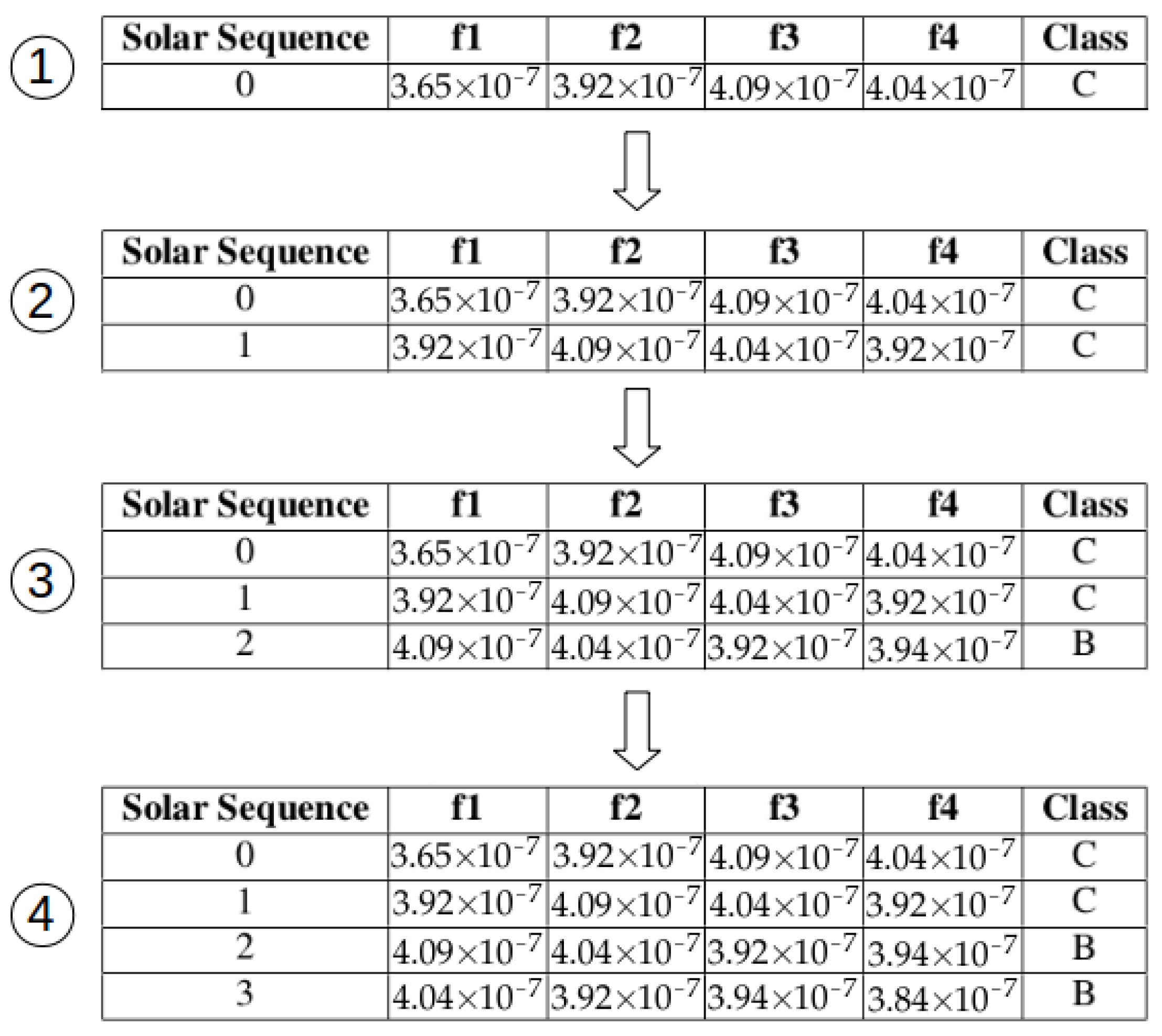
In line 5, SS builds a window starting in time instant t. The size of the window (windowSize) is the sum of the sizes of the current window, the jump and the future window. Then, in line 6, the first c values of the window is extracted and stored in an array called currentWindow. In line 7, the future window is generated using the f values obtained from the starting position of c + j within the window array and store in futureWindow. In line 8, maxSolarFlareClass receives the maximum solar flare found in the future window (futureWindow). In line 9, the Solar Sequence composed by the X-ray values of currentWindow and the maximum solar flare (maxSolarFlareClass) is built and stored in the array solarSequence. Line 10 adds the Solar Sequence of time instant t (solarSequence) in the final set of sequences SolarSequenceDataset. Line 12 returns the dataset with all the computed sequences called SolarSequenceDataset. Then, the next sequence is computed by returning processing to line 5. The number of windows and sequences built is set in the qty_of_windows variable. The sequential execution approach used in SS is shown in Figure 2.
In the sequential execution of SS, window-0 is fully built. Window-1 construction must wait for window-0 to be fully built. Similarly, windows 2 and 3 are generated waiting for their respective order in the sequential queue.
This example is tiny, but for large datasets, this processing model is very time-consuming because, depending on the input dataset size, the algorithm may face data processing of a Gigabyte order. Therefore, it is imperative to optimize SS.
For this purpose, it was developed a parallelized algorithm using GPU capabilities to optimize SS execution, making it more feasible to employ large datasets. The next section presents the parallelization strategy used in SS.
| Algorithm 1: The Series to Sequence (SS) algorithm. |
 |
3.1.2. Series to Sequence (SS) Algorithm: Parallel Version
The capabilities of GPUs architectures have been used to distribute the parallelized part of SS into threads executed in the CUDA cores of an NVIDIA enabled graphical card. The strategy used to parallelize SS was to execute the same instructions in different datasets within parallel threads.
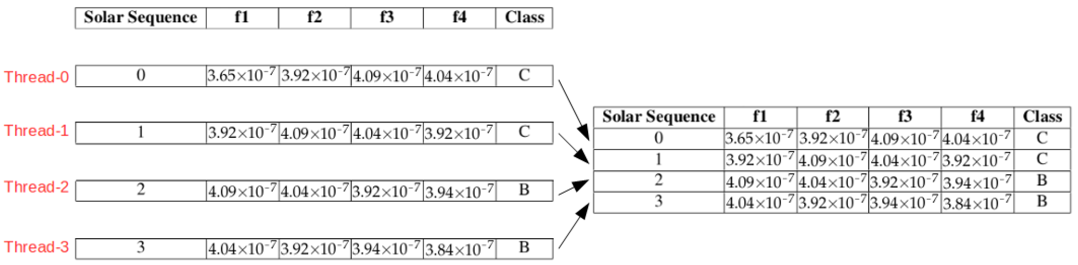
The instructions of SS executed in parallel are the ones responsible for the construction of each Solar Sequence. Moreover, the dataset used is the subsets of the X-ray times series that composed the full window (current window + jump + future window) of each step. The parallel execution approach used in SS is shown in Figure 3.
Each thread executed in the CUDA cores of the GPU builds one Solar Sequence individually and in parallel so that the construction of all Solar Sequence finishes approximately at the same time. As Figure 3 shows, Threads 0 to 3 are executed in parallel, and the full dataset (Solar Sequence Dataset) is also fulfilled in parallel.
In CUDA, a function called kernel is responsible for executing in parallel its instructions in the CUDA cores located at the NVIDIA GPU card. A function written in C and executed in the host computer is responsible for calling the kernel. Algorithm 2 presents the CUDA kernel algorithm of SS.
Algorithm 2 has as input the labeled X-ray time series, the current window, the step, the jump and the future window. The output is an array containing all the Solar Sequences called “SolarSequenceDataset”. This is the algorithm that the kernel function executes in GPU. Therefore, this algorithm is fired in parallel as many times as the number of windows, depending on the size of the X-ray time series and the window size. The resulting dataset (“SolarSequenceDataset”) will be fulfilled in the global memory of the GPU in parallel with all the sequences (“SolarSequence”) built by each fired thread. This is possible because each thread produces a unique index according to the order in which it was fired. This index can be used to obtain the array index of “SolarSequenceDataset” to place the SolarSequence built by the thread in its correct place in the array.
The threads running in the GPU are executed within a structure of blocks. A block, in CUDA, is a set of threads, so that the function in C that calls the kernel function must configure the number of threads per block and the number of blocks to correctly configure the parallel execution of SS. Line 2 contains the calculation of the index of the fired thread. This index is composed by the sum of the identifications of the fired thread (threadIdx.x), its block (blockIdx.x) and the number of threads per block (blockDim.x). Line 3 shows that the array index used to fulfill the “SolarSequenceDataset” (windowIndex) is calculated by multiplying the thread index obtained in Line 2 by the step value (s) given in the shift from one window to the other. Then, in line 6, it is decided if the thread will generate another Solar Sequence or not, depending if the windowIndex has reached the predefined number of windows or not. If so, lines 7 to 11 create the Solar Sequence according to the appropriate thread index, and line 12 adds the Solar Sequence to the SolarSequenceDataset in the correct place in the array through the calculated windowIndex.
Each NVIDIA GPU card has a maximum number of threads that may be executed within a block. In our case, we used the graphical card Geforce 960X, that can run up to 1024 threads per block. Therefore, the method was configured with 1024 threads per block, and the number of blocks was defined by Equation (1)
where:
| Algorithm 2: SS kernel function algorithm. |
 |
Equation (1) calculates the number of blocks because the number of windows may not be divisible by the NUMBEROFTHREADSPERBLOCK so that we have to guarantee that all of the windows will be handled by the fired threads.
The total number of windows that SS considers is given by subtracting the total size of the time series by the total window size and dividing this result by the step of instances between two adjacent windows.
Therefore, by using Algorithm 2 to implement the CUDA kernel function, it was possible to parallelize the creation of the Solar Sequence Dataset, as shown in the example of Figure 3.
4. Experiments
Three sets of experiments were performed to test SeMiner and its core algorithm, SS. The main goal of those experiments was to test two types of forecasting: forecasting of the X-ray background level emitted by the Sun, and forecasting of actual solar flares. Another goal was to test the effectiveness of the optimizations introduced in the parallel version of SS. An overview of these three sets of experiments are described as follows:
- The first set of experiments performed considered the intensity of X-rays in the 1–8 Angstrom band as input, generating a set of sequences. It is important to mention that it aimed to forecast the background level of X-ray flux instead of solar flare events. The method was tested using different classification methods and data size, forecasting one day in advance. The highest accuracy obtained in those tests was 91.3%. True Positive Rate was equal to 94.3%, while True Negative Rate was 86.5%, using the IBK classifier (a variation of the k-nearest neighbor method-KNN). These results show a strong balance between True Positive (TP) and True Negative (TN) rates, a desirable feature considering that the solar data relevant to this task is very imbalanced. It also corroborates that the KNN method may achieve near-optimal results in predicting future events given present values. These achievements can be found even in other application domains. As an example, the method of predicting demand for natural gas and energy cost savings described in [26] also employs KNN, obtaining results with very low error rates between estimated and performed events.
- In the second set of experiments, feature selection methods were applied. Relief Attribute Evaluation [27] and StarMiner [28] methods were employed in SeMiner to forecast actual solar flares and to select X-ray subseries belonging to the most relevant periods for solar flare forecasting. This approach resulted in good accuracy results, with balanced TP and TN rates, and achieved a high-performance speedup. The developed method achieved an accuracy of 72.7%, with a TP rate of 70.9% and TN rate of 79.7%. Another contribution of this work was the possibility to analyze the most significant X-ray subseries to consider in the forecasting method, considering that feature selection can help the task of choosing the best time intervals to be used by the forecasting module. In those experiments, it was found that the best time intervals to get an X-ray subseries was within two days for current observations, comprising both, the initial and final periods of the first day, and the remaining 16 h of the second day. This result corroborates the empirical opinion from the expert astrophysicist, who assumes that the analysis of two days of data is enough to predict possible future solar flares.
- The last set of experiments performed was concerned with the parallelized version of the SS algorithm. It was found that the optimized method developed in CUDA for execution using GPUs runs about four times faster than the original algorithm, developed in pure C language. Overall, the solution adopted exhibits good potential to optimize this kind of software application.
Details about each of those set of experiments are presented as follows, along with a discussion on the obtained results and main findings.
4.1. Experiment 1: X-ray Background Level Forecasting
SeMiner is prepared to use any data mining classification. Therefore, in this experiments, we employed the following classifiers to verify which one best forecasts X-ray flux intensity: J48 (a C4.5 implementation in Java), IBK (a k-nearest neighbor algorithm), Naive Bayes, OneR, and Support Vector Machine (SVM) using the Polykernel function as SVM kernel function. The implementations of these algorithms were taken from The Waikato Environment for Knowledge Analysis (WEKA) tool [29].
Accuracy, True Positive and True Negative rates were the metrics adopted to compare the obtained results. Furthermore, two types of dataset splitting were used to increase the results reliability:
- (1)
- 10 fold cross-validation: the dataset is divided into ten folds. Then, the first part is used as the test set, and the other nine as the training set. Afterwards, the second part is used as the test set, and the other nine as the training set, and so on.
- (2)
- Fixed dataset splitting: 67% for training, and 33% for testing.
Finally, the tests were performed using data taken from the following periods: 10 days, one month, one year and two years. The obtained results are presented as follows:
Table 5 shows the SeMiner experiments setup.
are validated with Cross-validation using 10 folds. On the other hand, and used of the data for training and the remaining for testing. The classes were categorized as “Yes”, for occurrences of the intensity of X-rays classified as C, M and X, and “No” otherwise. used data collected from a 10 days period, while used 30 days of data, used 60 days, used one year of data, and used 2 years of data containing X-ray flux intensity.
Accuracy, True Positive Rate and True Negative Rate were chosen because some tests resulted in high levels of accuracy, but a more throughout investigation has shown that though some tests had high accuracy, the data is unbalanced for one class, resulting in very low TN rate for one class. As the goal is to balance TPR and TNR in both classes (“maximum intensity event”: Yes and “no-maximum intensity event”: No), it was concluded that accuracy must be analyzed together with TP and TN.
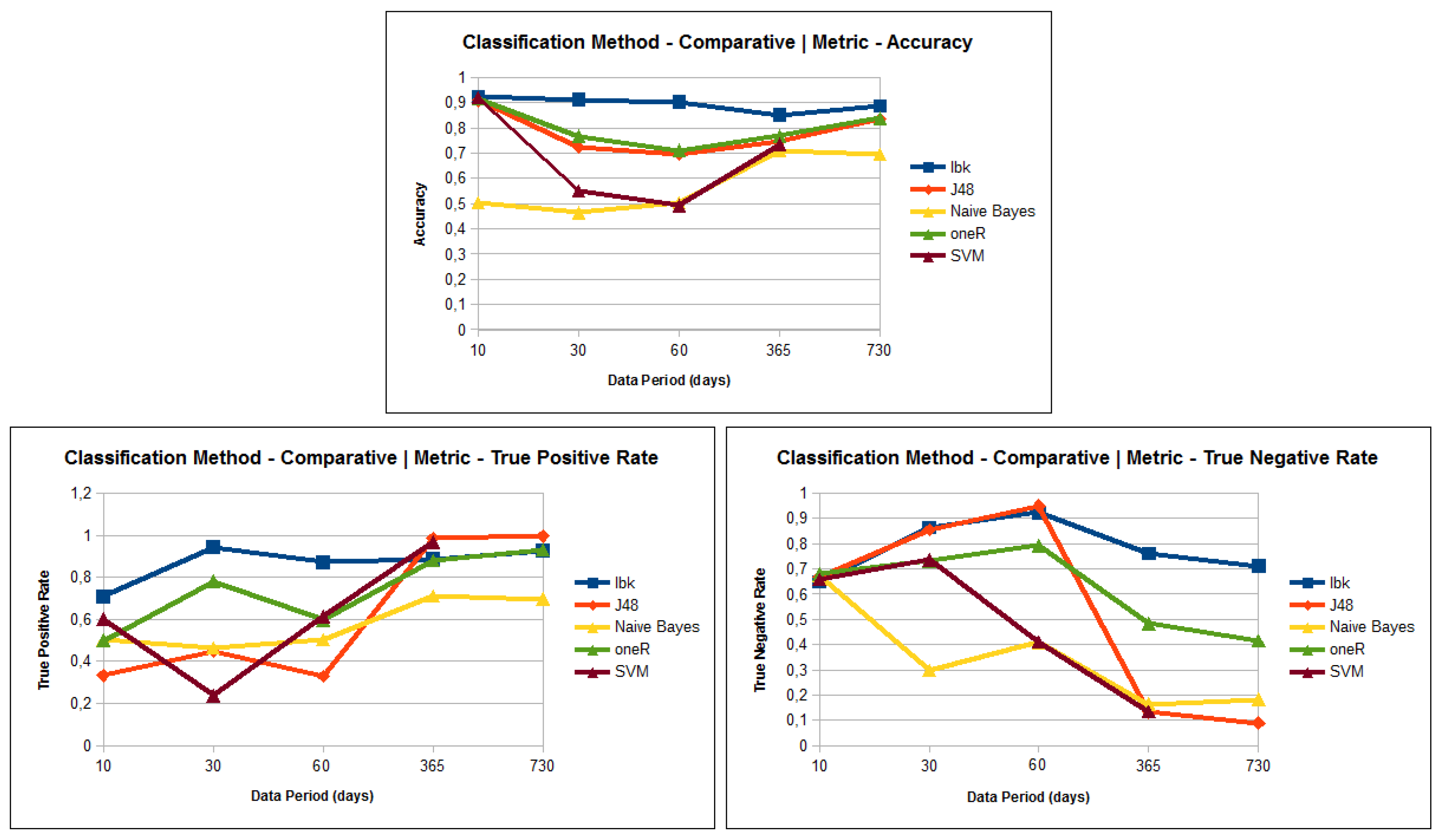
The graphics presented in Figure 4 shows the three metrics: Accuracy, True Positive Rate and True Negative Rate versus each test performed for 10, 30, 60, 365 and 730 days of data.
The results show three challenges to be faced: (1) the high unbalanced data nature; (2) the apparent high dimensionality characteristics of the processed data; (3) the decrease of TNR as the input data series increase.
Solar flare data is highly unbalanced because there is a much higher frequency of “No events” than “Yes events”.
Actually, the reported experiments have not worked with multidimensional data. The data series consist only of one-dimensional data, containing information about the intensity of the X-ray values. However, the sequencing process generates a multidimensional tuple of size n, which simulates a multidimensional data, even though the original dataset is unidimensional.
The decrease of TNR shows the loss of specificity of the method as the data size increases. In fact, as the data volume increase, the unbalanced data also increases. It improves the influence of the majority class in the learning model, making it less able to detect the minority class. This impacts negatively the TNR values. In fact, the challenge imposed by the unbalanced data must be faced with improvements in our method.
The classifier OneR was employed as the baseline classifier, which constructs one single rule for each data attribute. In spite of its simplicity, it performed relatively well (see Figure 4), because the input tuple was a preprocessed data sequence, with 288 attributes. In this case, the OneR model produced 288 rules that, using the majority vote strategy, could fairly describe the data.
The J48, also known as the C4.5 classifier, presented a significant decrease in the TN rate as the dataset size increased. It employs a Decision Tree approach that is very sensitive to an increase in the unbalanced data, losing the learning model specificity.
The use of Naive Bayes resulted in one of the poorest results. The method employs a probability model that assumes independence among attributes. However, the processed sequences have attributes with high levels of dependency.
Despite the fact that SVM usually produces good models to categorize tuples, it achieved poor results (accuracy: , TPR: and TNR: ) in the experiments performed. The SVM classifier presupposes a multidimensional data and finds the best hyperplanes that separate the data into classes. However, the datasets used are unidimensional, as previously discussed. Additionally, the computational performance of SVM is too low. was not completed using SVM as it took too long to complete.
The accuracy obtained using the IBK classification method was the highest one obtained in experiments. Thus, in most of the tests, IBK resulted in superior TPR and TNR results, which indicates that the results are balanced between classes Yes (maximum intensity event) and No (no-maximum intensity event). This result is related to the nature of IBK, which does not construct a learning model and also employs a distance function to compare tuples. The experiments showed that this “lazy” approach could achieve good results with the preprocessed data sequence. The test using 30 days of data achieved the best results when combining the three metrics: Accuracy (), TPR () and TNR ().
As the number of days considered in a dataset is a parameter of the method, and the domain specialist can refine the information given to the algorithm, the method tends to achieve better results. The specialist knowledge is an excellent source of information because he/she can inform: (1) the extension of the events (useful for setting up n); (2) the evolution of the events, so that parameter d can be properly informed; (3) the advance needed for the prediction (essential for setting up s and f parameters).
4.2. Experiment 2: Solar Flare Forecasting
The experiments performed for solar flare forecasting used data from 2014 to 2015, provided by “U.S. Department of Commerce, NOAA, Space Weather Prediction Center” at http://www.swpc.noaa.gov/products/goes-X-ray-flux using X-ray levels captured in a five-minute sample rate. X-ray flux emitted by Sun is monitored by two X-ray sensors located at the GOES (Geostationary Operational Environmental Satellite) satellite. The first sensor captures X-ray flux in the 0.5–4.0 Angstrom passband, while the other captures it in the 1–8 Angstrom passband. Solar flares are classified according to the intensity of X-ray in the 1 to 8 Angstroms passband.
The experiments were performed in three phases. First, the proposed method without feature selection was employed. In the second phase, “Starminer” was used for feature selection. Finally, in the third phase, “Relief Attribute Evaluation” was employed for this purpose. For each phase, X-ray time series from 2014 were used as the training dataset to produce a learning model with one day of forecasting advance. Then, the proposed method was tested employing data collected during six months of 2015.
A set of six experiments, divided into three phases, were performed to validate the proposed method as presented in Table 6. Those experiments were configured using the attributes described in Table 7:
Table 6 presents the configuration of the experiments performed:
Two main configurations were considered during each phase: (1) one day for the Current Window, and; (2) two days for the Current Window. Jump and Future Window were configured as one day for both phases. This means that the influence of X-rays for one day and two days were considered for the Current Window in the production of the forecasting model. The implementations of the classification methods were also obtained from the Weka tool [29]. The classification methods employed were: J48, IBK, Naive Bayes, OneR, Support Vector Machine [30,31,32,33,34].
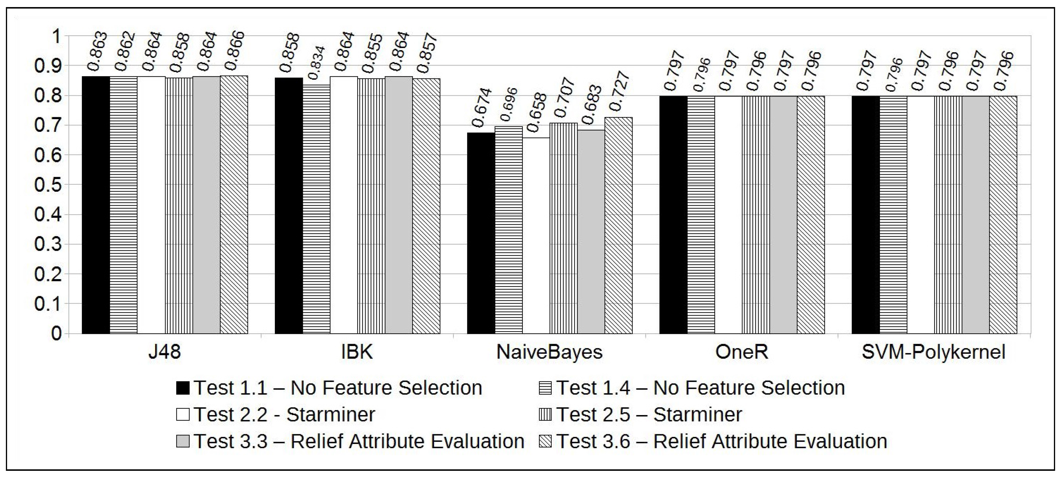
The experiments resulted in high accuracy rates for the majority of the classification methods (see Figure 5). However, a deeper analysis of the results showed that the majority of the classification methods also resulted in high differences between the True Positive and True Negative rates. As already said, this difference is due to the unbalanced characteristic of the solar flare time series, since high-intensity solar flares are rare. For that reason, the ROC (Receiver Operating Characteristic) area information [35] was adopted to qualify the method efficacy. The largest ROC Area indicates the best results obtained, suggesting the best and most balanced results for accuracy, TP, and TN rates.
As we can see in Figure 6, the Naive Bayes classifier resulted in the largest ROC areas. Notably, Test 3.6 has the largest one, reaching 0.799 of the ROC area. On the other hand, we observe that this experiment got an accuracy of 72.7%. This accuracy can be considered high, considering the unbalanced dataset, and is accompanied by balanced TP and TN rates, 70.9% and 79.7%, respectively.
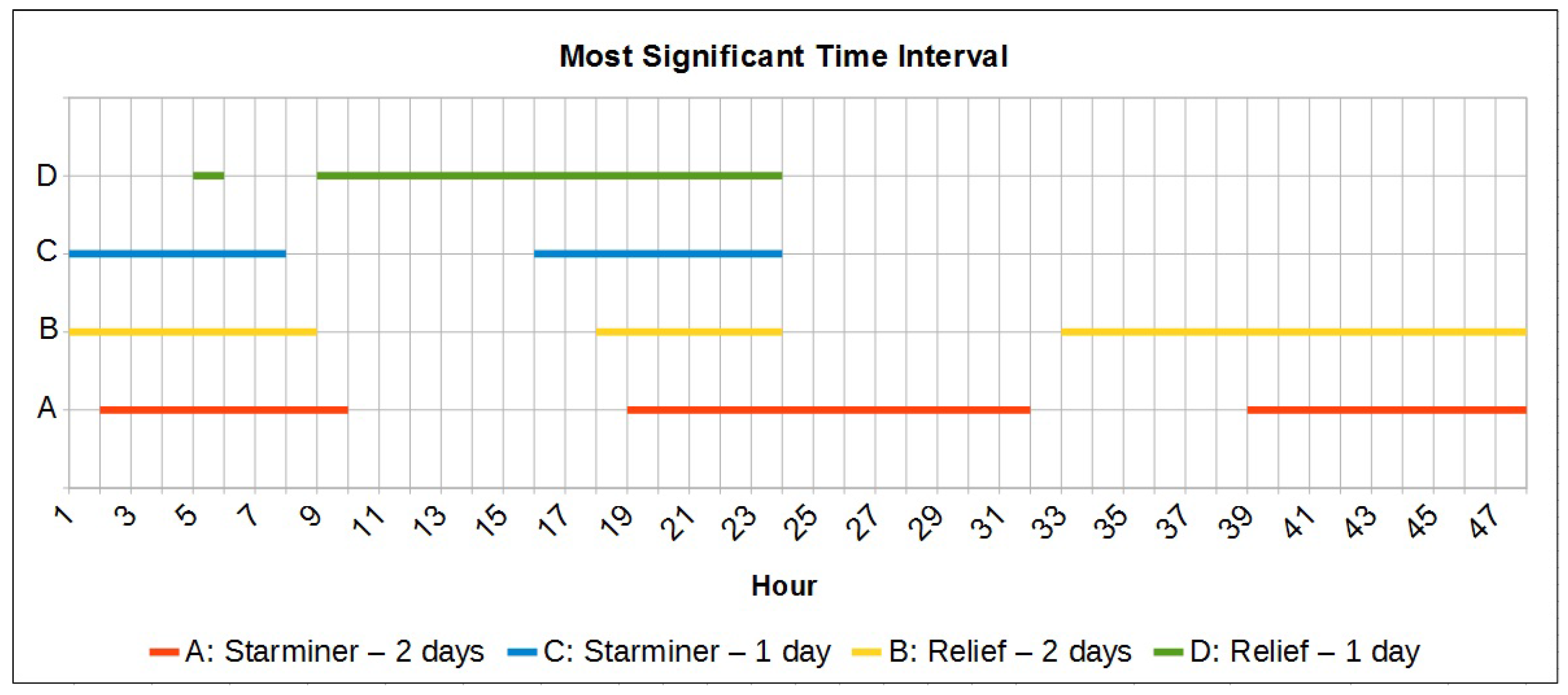
Test 3.6 results were also significant for some reasons: (1) as shown in Table 6, Test 3.6 is configured with a “current window” of 2 days and, according to the domain specialist, this time period has the most significant pattern that can be observed to forecast a solar flare; (2) if “Relief Attribute Selection” is used, along with a two days time period for the “current window”, the most significant instants to use in the forecasting model are comprised in the following intervals (given in hours): (start of the first day), (end of the first day), and (last 16 h of the second day); (3) feature selection along with the Naive Bayes classifier resulted in the best accuracy and ROC area among all the tests performed. Furthermore, it resulted in a speedup of 3.2, i.e., an execution time 3.2 faster than if all features of the dataset were considered (); (4) the overall accuracy, considering the tests performed with 2 days of “current window", increased from 69.6% (without feature selection) to 72.7% (using feature selection). Also, the ROC Area was increased from 0.768 to 0.799.
To better illustrate the obtained results, the analysis of the most significant periods to consider is shown in Figure 8.
4.3. Experiment 3: SS Parallel Optimizations
Two sets of experiments were performed to compare the parallel version of the SS algorithm against its sequential implementation.
The first set of experiments was performed using the implementation based on pure C language, and a three years time series of X-ray intensity data (2013 to 2015). The Current Window, Jump and Future Window were set to 288 instances, while Step was set to one instance. As the sample rate is 5 min, it is equivalent to say that Current Window, Jump and Future Window are set to one day. Thus, the intended forecasting was done for one day in advance. The running times of interest were measured using the “time” command of C and CUDA, and the start/end of the “time” command involved just the function that executed the pure C algorithm. The pure C algorithm was run three times, and its mean execution time was calculated.
The second set of experiments was performed with the same configuration of the previous one, except that the CUDA kernel implementation was used. In this experiment, the “time” command of C and CUDA was also used, but the start/end was concerned with the parallelized function. Thus, it measured the sum of all the threads fired. The kernel function was run three times and its mean execution time was calculated.
A summary of the experiments, the mean execution time and the processed data size are shown in Table 8.
All the experiments were performed on a computer with the following hardware configuration:
- Processor: Intel i5;
- RAM: 8 GB;
- Graphic’s card: Geforce 960X
- -
- Number of CUDA cores (GPUs): 1024
- -
- Memory: 2 GB
- Operating System: Windows 10;
- Application running during the test: Eclipse IDE
The execution speedup obtained by using CUDA for the implementation of SS is presented in Equation (2):
Considering the reported experiments, the algorithm implemented using CUDA showed to be 4.36 times faster than the implementation using pure C, producing the same output of the sequential version.
5. Method Limitations and Future Directions
Depending on the forecasting horizons range, three types of forecasting are possible: (1) short-term forecasting: embraces horizons of hours/days; (2) medium-term forecasting: includes horizons of months; (3) long-term forecasting: includes horizons of years. The method described in this paper is targeted to short-term forecasting. Therefore, further experiments should be performed to test medium and long-term forecasting. In this way, the main limitations of the presented method regarding forecasting horizons are:
- (a)
- There is no consensus in solar space research regarding which set of solar features fully describe the events that determine the occurrence of solar flares and changes in the X-ray background level emitted by the Sun. In the method described in this paper, we have used the X-ray levels emitted by the Sun to predict future solar events. However, other works have considered different aspects, such as magnetic features captured from the Sun, or even features related to the geometry of sunspots found in the Sun chromosphere layer. Therefore, we intend to improve our method by using other features, expecting to increase the accuracy for longer forecasting horizons;
- (b)
- Other limitation of our method resides in the fact that, for the optimized version, it relies on a single server with just one GPU card. Considering the characteristics of the adopted parallel implementation, this architecture limits the data size the method can handle, which limits the time series length. One of the future aims of this project is to use data from at least eleven years, as this period encompass one full solar cycle, and may produce a learning model more suitable for middle or long-term forecasting. One solar cycle is the period upon which the solar activity increases to a top level and regresses to the weakest level. Implementation changes in the parallel version of the algorithm, or even a more powerful parallel architecture should allow us to fully exploit a much larger dataset, and maybe better results for longer forecasting horizons;
- (c)
- The third limitation of our method is that, as the size of the window increases, the method turns more demanding regarding computing time. Thus, as the forecasting horizon increases, the time for building the prediction model also increases;
- (d)
- Finally, according to astrophysicists’ empirical findings, the analysis of the last two days of X-ray flux may indicate a possible solar event within a maximum horizon of 3 days. Our method was developed based on this observation so that if the horizon exceeds three days, the method accuracy decreases.
It is important to observe that, at this point, the goal of the domain specialist of our project, is to get an accurate model for short-term forecasting, so the “SeMiner" method has been developed for this specific requirement.
Regarding future work, we intend to consider other solar features than X-ray levels to SeMiner, aiming to improve the method accuracy and the forecasting horizon. We also intend to improve the optimization method to allow it to use a dataset of one full solar cycle as well as enable the method to run larger windows.
6. Conclusions
This work has been developed in the context of sun X-Ray flux emissions, and solar flare predictions. The SeMiner forecasting method has been developed and tested using a number of strategies aiming to improve parameters such as accuracy, true positive and true negative rates.
More specifically, this paper presents our approach to deal with a crucial step in the process of forecasting solar flares and X-ray background level: the data mining preprocessing step using specialist knowledge from domain experts.
In the first set of experiments, SeMiner was used to predict the background level of X-ray flux emitted by the Sun. The method was tested using different classification methods and data sizes. The best results obtained achieved an accuracy of 91.3%, True Positive Rate of 94.3% and True Negative Rate of 86.5% using IBK. These results firmly balance True Positive and True Negative rates, which is an essential issue because solar data is quite unbalanced.
In the second set of experiments, the historical evolution of an X-ray time series was considered to produce the forecasting model. Furthermore, feature selection methods such as “Starminer” and “Relief Attribute Evaluation” were used to obtain an analysis of the most significant periods of time to be considered by the forecasting method. This approach resulted in high accuracy results, with balanced TP and TN rates. The strategy also resulted in some optimization in terms of execution speed, as the adoption of feature selection resulted in a performance speedup of 3.2. Those experiments reached an accuracy of 72.7%, with a TP rate of 70.9% and TN rate of 79.7%.
Another contribution of this work was the analysis aiming to identify the most significant time intervals to consider the forecasting method. It was concluded that, in the scope of our experiments, the best time interval was within two days for “current window” and comprised both, the initial and end periods of the first day, and the last 16 h of the second day. This result corroborates the theory from domain specialists that the analysis of two days of data can determine possible future Solar Flares.
Finally, the third set of experiments was concerned with further performance optimizations. The core module of SeMiner, the SS algorithm, was parallelized using CUDA, targeting parallel execution in GPUs. The strategy showed to be 4.36 times faster than its pure C sequential version.
These results indicate that the SeMiner method is well-suited to predict X-ray background level and solar flare.
Acknowledgments
We acknowledge INPE (Brazilian National Institute for Space Research) specialists which support us with their solar knowledge, and Federal Institute of São Paulo for supporting the PhD student conducting this research effort.
Author Contributions
Sérgio Luisir Díscola Junior conceived and developed the methods “SeMiner” and “SS”. Marcela Xavier Ribeiro and Márcio Merino Fernandes analyzed the computational concepts of the methods. Sérgio Luisir Díscola Junior conceived and run the experiments. Sérgio Luisir Díscola Junior, Marcela Xavier Ribeiro and Márcio Merino Fernandes analyzed the results in the computational view point. José Roberto Cecatto analyzed the results in the astrophysicial view point. Sérgio Luisir Díscola Junior, Marcela Xavier Ribeiro, Márcio Merino Fernandes and José Roberto Cecatto wrote and reviewed the paper. José Roberto Cecatto contributed as the domain specialist providing support, examples, materials and tools regarding the solar events described in the paper. All authors have read and approved the final manuscript.
Conflicts of Interest
The authors declare no conflict of interest.
References
- Tsurutani, B.T.; Verkhoglyadova, O.P.; Mannucci, A.J.; Lakhina, G.S.; Li, G.; Zank, G.P. A brief review of “solar flare effects” on the ionosphere. Radio Sci. 2009, 44. [Google Scholar] [CrossRef]
- Basu, S.; Basu, S.; MacKenzie, E.; Bridgwood, C.; Valladares, C.E.; Groves, K.M.; Carrano, C. Specification of the occurrence of equatorial ionospheric scintillations during the main phase of large magnetic storms within solar cycle 23. Radio Sci. 2010, 45, 1–15. [Google Scholar] [CrossRef]
- Winter, L.M.; Balasubramaniam, K. Using the maximum X-ray flux ratio and X-ray background to predict solar flare class. Space Weather 2015, 13, 286–297. [Google Scholar] [CrossRef]
- McIntosh, P.S. The classification of sunspot groups. Sol. Phys. 1990, 125, 251–267. [Google Scholar] [CrossRef]
- Gallagher, P.T.; Moon, Y.J.; Wang, H. Active-Region Monitoring and Flare Forecasting—I. Data Processing and First Results. Sol. Phys. 2002, 209, 171–183. [Google Scholar] [CrossRef]
- Barnes, G.; Leka, K.D.; Schumer, E.A.; Della-Rose, D.J. Probabilistic forecasting of solar flares from vector magnetogram data. Space Weather 2007, 5. [Google Scholar] [CrossRef]
- Ahmed, O.W.; Qahwaji, R.; Colak, T.; Higgins, P.A.; Gallagher, P.T.; Bloomfield, D.S. Solar Flare Prediction Using Advanced Feature Extraction, Machine Learning, and Feature Selection. Sol. Phys. 2013, 283, 157–175. [Google Scholar] [CrossRef]
- Nishizuka, N.; Sugiura, K.; Kubo, Y.; Den, M.; Watari, S.; Ishii, M. Solar Flare Prediction Model with Three Machine-learning Algorithms using Ultraviolet Brightening and Vector Magnetograms. Astrophys. J. 2017, 835, 156. [Google Scholar] [CrossRef]
- Bobra, M.G.; Couvidat, S. Solar Flare Prediction Using SDO/HMI Vector Magnetic Field Data with a Machine-Learning Algorithm. Astrophys. J. 2015, 798, 135. [Google Scholar] [CrossRef]
- Li, R.; Zhu, J. Solar flare forecasting based on sequential sunspot data. Res. Astron. Astrophys. 2013, 13, 1118–1126. [Google Scholar] [CrossRef]
- Yu, D.; Huang, X.; Hu, Q.; Zhou, R.; Wang, H.; Cui, Y. Short-Term Solar Flare Prediction Using Multiresolution Predictors. Astrophys. J. 2010, 709, 321–326. [Google Scholar] [CrossRef]
- Zavvari, A.; Islam, M.T.; Anwar, R.; Abidin, Z.Z. Solar Flare M-Class Prediction Using Artificial Intelligence Techniques. J. Theor. Appl. Inf. Technol. 2015, 74, 63–67. [Google Scholar]
- Qahwaji, R.; Colak, T. Automatic Short-Term Solar Flare Prediction Using Machine Learning and Sunspot Associations. Sol. Phys. 2007, 241, 195–211. [Google Scholar] [CrossRef] [Green Version]
- Wang, H.; Cui, Y.; Li, R.; Zhang, L.; Han, H. Solar flare forecasting model supported with artificial neural network techniques. Adv. Space Res. 2008, 42, 1464–1468. [Google Scholar] [CrossRef]
- Zhang, X.; Liu, J.; Wang, Q. Image feature extraction for solar flare prediction. In Proceedings of the 2011 4th International Congress on Image and Signal, Shanghai, China, 15–17 October 2011; pp. 910–914. [Google Scholar]
- Huang, X.; Yu, D.; Hu, Q.; Wang, H.; Cui, Y. Short-Term Solar Flare Prediction Using Predictor Teams. Sol. Phys. 2010, 263, 175–184. [Google Scholar] [CrossRef]
- Yu, D.; Huang, X.; Wang, H.; Cui, Y. Short-Term Solar Flare Prediction Using a Sequential Supervised Learning Method. Sol. Phys. 2009, 255, 91–105. [Google Scholar] [CrossRef]
- Yuan, Y.; Shih, F.Y.; Jing, J.; Wang, H.M. Automated flare forecasting using a statistical learning technique. Res. Astron. Astrophys. 2010, 10, 785–796. [Google Scholar] [CrossRef]
- Colak, T.; Qahwaji, R. Automated Solar Activity Prediction: A hybrid computer platform using machine learning and solar imaging for automated prediction of solar flares. Space Weather 2009, 7. [Google Scholar] [CrossRef]
- Innocenti, M.E.; Johnson, A.; Markidis, S.; Amaya, J.; Deca, J.; Olshevsky, V.; Lapenta, G. Progress towards physics based space weather forecasting with exascale computing. Adv. Eng. Softw. 2017, 111, 3–17. [Google Scholar] [CrossRef]
- Wells, B.E.; Singh, N.; Somarouthu, T. Parallel kinetic particle in cell code simulation of astrophysical plasmas affecting magnetic reconnection (non-reviewed). In Proceedings of the IEEE SoutheastCon 2008, Huntsville, AL, USA, 3–6 April 2008; p. 261. [Google Scholar]
- Volberg, O.; Toth, G.; Gombosi, T.I.; Stout, Q.F.; Powell, K.G.; De Zeeuw, D.; Ridley, A.J.; Kane, K.; Hansen, K.C.; Chesney, D.R.; et al. A high performance framework for sun to earth space weather modeling. In Proceedings of the 19th IEEE International Parallel and Distributed Processing Symposium (IPDPS), Denver, CO, USA, 4–8 April 2005. [Google Scholar]
- Clauer, C.R.; Gombosi, T.I.; Zeenw, D.L.D.; Ridley, A.J.; Powell, K.G.; Leer, B.V.; Stout, Q.F.; Groth, C.P.T.; Holzer, T.E. High performance computer methods applied to predictive space weather simulations. IEEE Trans. Plasma Sci. 2000, 28, 1931–1937. [Google Scholar] [CrossRef]
- Poli, G.; Llapa, E.; Cecatto, J.; Saito, J.; Peters, J.; Ramanna, S.; Nicoletti, M. Solar flare detection system based on tolerance near sets in a GPU CUDA framework. Knowl. Based Syst. 2014, 70, 345–360. [Google Scholar] [CrossRef]
- Xenopoulos, P.; Daniel, J.; Matheson, M.; Sukumar, S. Big data analytics on HPC architectures: Performance and cost. In Proceedings of the 2016 IEEE International Conference on Big Data (Big Data), Washington, DC, USA, 5–8 December 2016; pp. 2286–2295. [Google Scholar]
- Rodger, J.A. A fuzzy nearest neighbor neural network statistical model for predicting demand for natural gas and energy cost savings in public buildings. Expert Syst. Appl. 2014, 41, 1813–1829. [Google Scholar] [CrossRef]
- Kira, K.; Rendell, L.A. A practical approach to feature selection. In Proceedings of the ninth international workshop on Machine learning, Aberdeen, UK, 1–3 July 1992; pp. 249–256. [Google Scholar]
- Ribeiro, M.X.; Balan, A.G.R.; Felipe, J.C.; Traina, A.J.M.; Traina, C. Mining statistical association rules to select the most relevant medical image features. In Mining Complex Data; Springer: Berlin/Heidelberg, Germany, 2009; pp. 113–131. [Google Scholar]
- Hall, M.; Frank, E.; Holmes, G.; Pfahringer, B.; Reutemann, P.; Witten, I. The WEKA data mining software: An update. SIGKDD Explor. 2009, 11, 10–18. [Google Scholar] [CrossRef]
- Quinlan, J.R.; Ross, J. C4.5: Programs for machine learning; Morgan Kaufmann Publishers: Burlington, MA, USA, 1993; p. 302. [Google Scholar]
- Aha, D.W.; Kibler, D.; Albert, M.K. Instance-Based Learning Algorithms. Mach. Learn. 1991, 6, 37–66. [Google Scholar] [CrossRef]
- Besnard, P.; Hanks, S. Uncertainty in Artificial Intelligence: Proceedings of the Eleventh Conference (1995): 18–20 August 1995; Morgan Kaufmann Publishers: San Francisco, CA, USA, 1995; p. 591. [Google Scholar]
- Holte, R.C. Very Simple Classification Rules Perform Well on Most Commonly Used Datasets. Mach. Learn. 1993, 11, 63–90. [Google Scholar] [CrossRef]
- Schoolkopf, B.; Burges, C.J.C.; Smola, A.J. Advances in Kernel Methods: Support Vector Learning; MIT Press: Cambridge, MA, USA, 1999; p. 376. [Google Scholar]
- Fawcett, T. ROC Graphs: Notes and Practical Considerations for Researchers; Technical Report; HP Laboratories: Palo Alto, CA, USA, 2004. [Google Scholar]
Figure 1.
SeMiner: Method Overview.
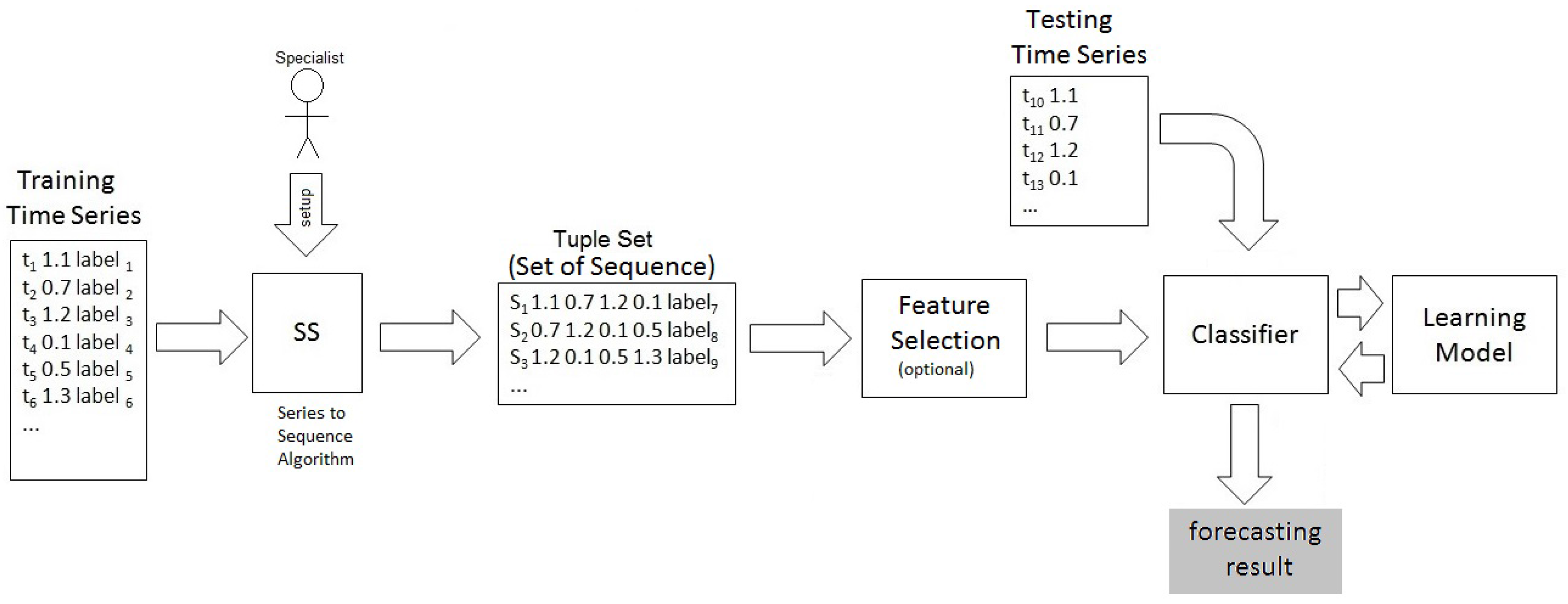
Figure 2.
Illustration of the sequential execution approach used in SS.

Figure 3.
Illustration of the parallel execution approach used in SS.

Figure 4.
Results of the first set of experiments.

Figure 5.
Accuracy.

Figure 6.
ROC Area.
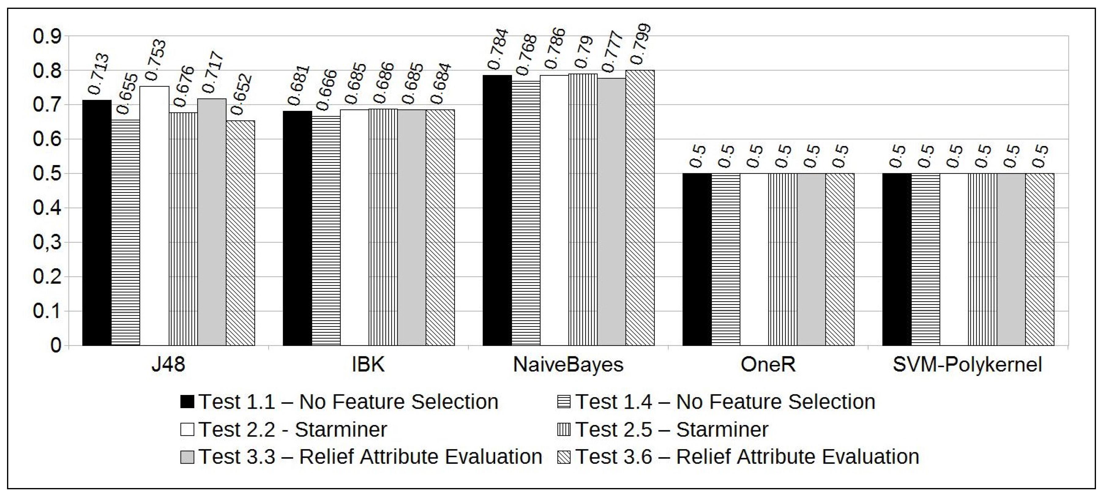
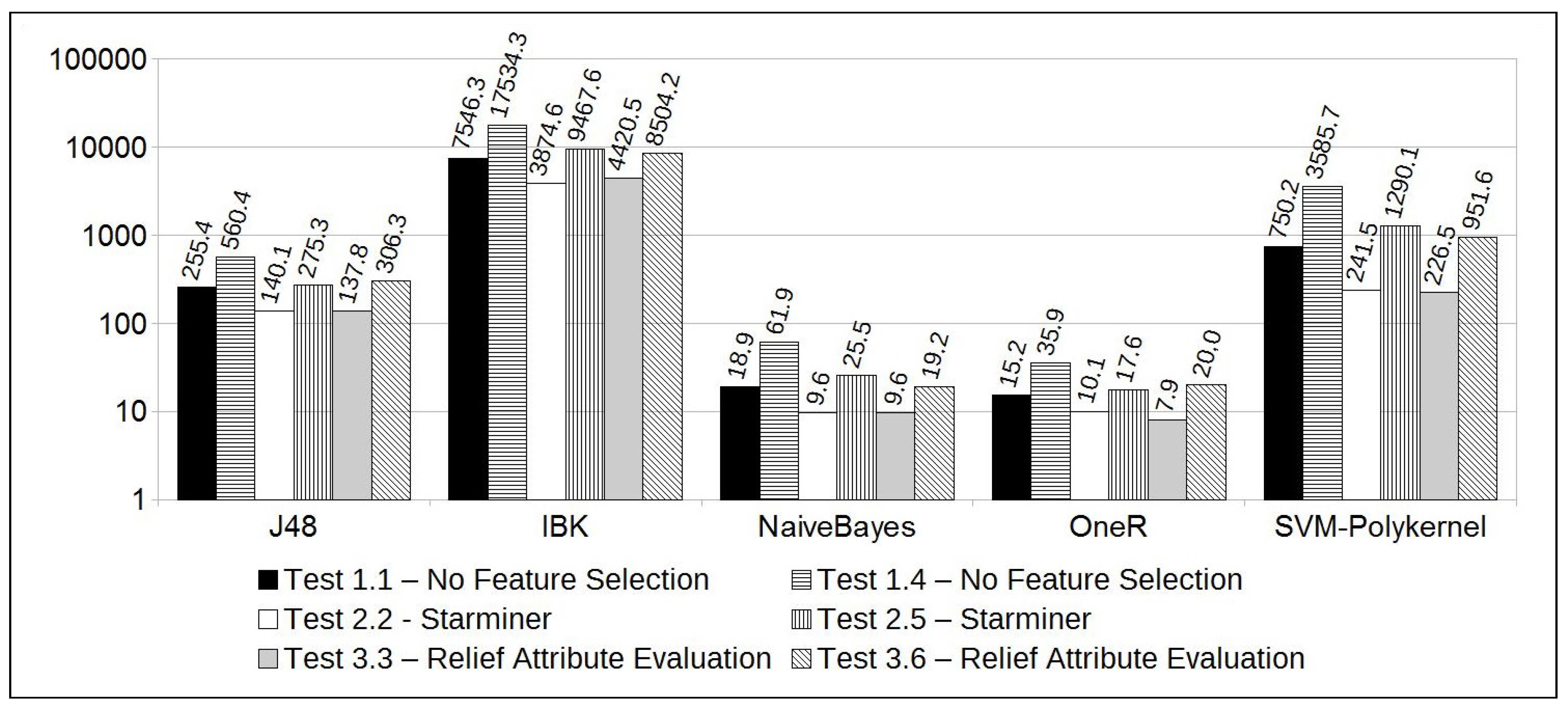
Figure 7.
Total time = Training Time + Testing Time (Time in seconds).

Figure 8.
Most significant time interval analysis.


Table 1.
Example of dataset tuples-XTS(t).
| X-ray Time Series | Solar Flare Class | |
|---|---|---|
| t | X(t) | |
| 0 | 3.65 × 10 | B |
| 5 | 3.92 × 10 | B |
| 10 | 4.09 × 10 | B |
| 15 | 4.04 × 10 | B |
| 20 | 3.92 × 10 | B |
| 25 | 3.94 × 10 | B |
| 30 | 3.84 × 10 | B |
| 35 | 3.80 × 10 | B |
| 40 | 3.80 × 10 | B |
| 45 | 3.83 × 10 | C |
| 50 | 3.84 × 10 | B |
| 55 | 3.90 × 10 | B |
| 60 | 6.47 × 10 | B |
| 65 | 6.75 × 10 | B |
| 70 | 5.24 × 10 | B |
Table 2.
Sliding window evolution performed in the execution of SS.
| X-ray Time Series | ||||||
| t | X(t) | Class of Solar Flare | Window-0 | Window-1 | ||
| 0 | 3.65 | B | Current-Window | step | Window-2 | |
| 5 | 3.92 | B | Current-Window | step | Window-3 | |
| 10 | 4.09 | B | Current-Window | step | ||
| 15 | 4.04 | B | Current-Window | |||
| 20 | 3.92 | B | jump | |||
| 25 | 3.94 | B | jump | |||
| 30 | 3.84 | B | jump | |||
| 35 | 3.80 | B | jump | |||
| 40 | 3.80 | B | Future-Window | |||
| 45 | 3.83 | C | Future-Window | |||
| 50 | 3.84 | B | Future-Window | |||
| 55 | 3.90 | B | Future-Window | |||
| 60 | 6.47 | B | ||||
| 65 | 6.75 | B | ||||
| 70 | 5.24 | B |
Table 3.
Example of the values of the windows built in SS.
| Current Window (f1–f4) | Jump (f5–f8) | Future Window (f9–f12) | ||||||||||
|---|---|---|---|---|---|---|---|---|---|---|---|---|
| Window | f1 | f2 | f3 | f4 | f5 | f6 | f7 | f8 | f9 | f10 | f11 | f12 |
| 0 | 3.65 (B) | 3.92 (B) | 4.09 (B) | 4.04 (B) | 3.92 (B) | 3.94 (B) | 3.84 (B) | 3.80 (B) | 3.80 (B) | 3.83 (C) | 3.84 (B) | 3.90 (B) |
| 1 | 3.92 (B) | 4.09 (B) | 4.04 (B) | 3.92 (B) | 3.94 (B) | 3.84 (B) | 3.80 (B) | 3.80 (B) | 3.83 (C) | 3.84 (B) | 3.90 (B) | 6.47 (B) |
| 2 | 4.09 (B) | 4.04 (B) | 3.92 (B) | 3.94 (B) | 3.84 (B) | 3.80 (B) | 3.80 (B) | 3.83 (C) | 3.84 (B) | 3.90 (B) | 6.47 (B) | 6.75 (B) |
| 3 | 4.04 (B) | 3.92 (B) | 3.94 (B) | 3.84 (B) | 3.80 (B) | 3.80 (B) | 3.83 (C) | 3.84 (B) | 3.90 (B) | 6.47 (B) | 6.75 (B) | 5.24 (B) |
Table 4.
Example of a “Solar Sequence Dataset (SSD)”.
| Solar Sequence | f1 | f2 | f3 | f4 | Class |
|---|---|---|---|---|---|
| 0 | 3.65 | 3.92 | 4.09 | 4.04 | C |
| 1 | 3.92 | 4.09 | 4.04 | 3.92 | C |
| 2 | 4.09 | 4.04 | 3.92 | 3.94 | B |
| 3 | 4.04 | 3.92 | 3.94 | 3.84 | B |
Table 5.
Setup of the SeMiner experiments. Test ID is the number of the performed experiment; n (current window size), d (window step), s (jump) and f (size of the future window) are measured in numbers of observations; (period of time) is measured in minutes; is the number of generated sequences.
Table 5.
Setup of the SeMiner experiments. Test ID is the number of the performed experiment; n (current window size), d (window step), s (jump) and f (size of the future window) are measured in numbers of observations; (period of time) is measured in minutes; is the number of generated sequences.
| Test ID | Test and Training Set Division Method | Class Definition of Solar Event | n | s | f | d | #Observations | Data Period (Days) | ||
|---|---|---|---|---|---|---|---|---|---|---|
| 1 | Cross-validation: 10 folds | C, M and X | 5 | 288 | 288 | 288 | 1 | 2880 | 10 | 2016 |
| 2 | Cross-validation: 10 folds | C, M and X | 5 | 288 | 288 | 288 | 1 | 8640 | 30 | 7776 |
| 3 | Cross-validation: 10 folds | C, M and X | 5 | 288 | 288 | 288 | 1 | 17,280 | 60 | 16,416 |
| 4 | Percentage split: 67% for training data | C, M and X | 5 | 288 | 288 | 288 | 1 | 105,120 | 365 | 104,256 |
| 5 | Percentage split: 67% for training data | C, M and X | 5 | 288 | 288 | 288 | 1 | 210,240 | 730 | 209,376 |
Table 6.
Experiments Planning.
| Phase. Test Id | Feature Selection Method | Current Window | Jump | Future Window | Data Interval | Classification Method | |
|---|---|---|---|---|---|---|---|
| Training | Testing | ||||||
| 1.1 | Not used | 1 | 1 | 1 | 1 year 2014 | 6 months 2015 | J48, IBK, NaiveBayes, OneR, SVM (Weka-SMO-Polykernel) |
| 2.2 | Starminer | ||||||
| 3.3 | Relief Attribute Evaluation | ||||||
| 1.4 | Not used | 2 | 1 | 1 | |||
| 2.5 | Starminer | ||||||
| 3.6 | Relief Attribute Evaluation | ||||||
Table 7.
Description of the attributes used in the experiments.
| Configuration Attribute | Description | Possible Values |
|---|---|---|
| Feature Selection | This attribute tells the Feature Selection Method used | Not used Starminer Relief Attribute Evaluation |
| Current window | This attribute tells the number of days of the window used to compose the sequence that will be labeled with the “future” class. | Integer value |
| Jump | This attribute tells the number of observations that will be considered to build the next sequence. | Integer value |
| Future window | This attribute tells the number of days of the window used to look for the “future” class of the previouly defined “Current window” | Integer value |
| Data Interval/Training | This attribute tells the interval considered to catch the data used during the training phase of the classification method used in the experiments. | 1 year 2014 |
| Data Interval/Testing | This attribute tells the interval considered to catch the data used during the testing phase of the experiments. | 6 months 2015 |
| Classification Method | This attribute tells the Data Mining Classification Method used during the validation of the proposed forecasting method. | J48, IBK, NaiveBayes, OneR SVM (Weka-SMO-Polykernel) |
Table 8.
SS CUDA implementation: Experiments and Results.
| Setup | Results | ||||||
|---|---|---|---|---|---|---|---|
| Seminer Implementation | Data Volume | Current Window | Jump | Future Window | Step | Mean Execution Time (s) | Size of Output File |
| pure C | 3 years (2013–2015) | 288 | 288 | 288 | 1 | 208.5 | 1.09 GB |
| With CUDA | 3 years (2013–2015) | 288 | 288 | 288 | 1 | 47.8 | 1.09 GB |
© 2018 by the authors. Licensee MDPI, Basel, Switzerland. This article is an open access article distributed under the terms and conditions of the Creative Commons Attribution (CC BY) license (http://creativecommons.org/licenses/by/4.0/).
Share and Cite
MDPI and ACS Style
Díscola Junior, S.L.; Cecatto, J.R.; Merino Fernandes, M.; Xavier Ribeiro, M. SeMiner: A Flexible Sequence Miner Method to Forecast Solar Time Series. Information 2018, 9, 8. https://doi.org/10.3390/info9010008
AMA Style
Díscola Junior SL, Cecatto JR, Merino Fernandes M, Xavier Ribeiro M. SeMiner: A Flexible Sequence Miner Method to Forecast Solar Time Series. Information. 2018; 9(1):8. https://doi.org/10.3390/info9010008
Chicago/Turabian StyleDíscola Junior, Sérgio Luisir, José Roberto Cecatto, Márcio Merino Fernandes, and Marcela Xavier Ribeiro. 2018. "SeMiner: A Flexible Sequence Miner Method to Forecast Solar Time Series" Information 9, no. 1: 8. https://doi.org/10.3390/info9010008
Note that from the first issue of 2016, this journal uses article numbers instead of page numbers. See further details here.