Article

sCwc/sLcc: Highly Scalable Feature Selection Algorithms

1
Graduate School of Applied Informatics, University of Hyogo, Kobe 651-2197, Japan
2
Information Networking Institute, Carnegie Mellon University, Pittsburgh, PA 15213, USA
3
Computer Centre, Gakushuin University, Tokyo 171-0031, Japan
4
Institude of Economic Research, Chiba University of Commerce, Chiba 272-8512, Japan
5
Center for Digital Humanities, University of California Las Angeles; Los Angeles, CA 90095, USA
*
Author to whom correspondence should be addressed.
These authors contributed equally to this work.
Information 2017, 8(4), 159; https://doi.org/10.3390/info8040159
Submission received: 31 October 2017 / Revised: 1 December 2017 / Accepted: 2 December 2017 / Published: 6 December 2017
(This article belongs to the Special Issue Feature Selection for High-Dimensional Data)

Abstract

:
Feature selection is a useful tool for identifying which features, or attributes, of a dataset cause or explain the phenomena that the dataset describes, and improving the efficiency and accuracy of learning algorithms for discovering such phenomena. Consequently, feature selection has been studied intensively in machine learning research. However, while feature selection algorithms that exhibit excellent accuracy have been developed, they are seldom used for analysis of high-dimensional data because high-dimensional data usually include too many instances and features, which make traditional feature selection algorithms inefficient. To eliminate this limitation, we tried to improve the run-time performance of two of the most accurate feature selection algorithms known in the literature. The result is two accurate and fast algorithms, namely sCwc and sLcc. Multiple experiments with real social media datasets have demonstrated that our algorithms improve the performance of their original algorithms remarkably. For example, we have two datasets, one with 15,568 instances and 15,741 features, and another with 200,569 instances and 99,672 features. sCwc performed feature selection on these datasets in 1.4 seconds and in 405 seconds, respectively. In addition, sLcc has turned out to be as fast as sCwc on average. This is a remarkable improvement because it is estimated that the original algorithms would need several hours to dozens of days to process the same datasets. In addition, we introduce a fast implementation of our algorithms: sCwc does not require any adjusting parameter, while sLcc requires a threshold parameter, which we can use to control the number of features that the algorithm selects.

1. Introduction

Accurate and fast feature selection is a useful tool of data analysis. In particular, feature selection on categorical data is important in real world applications. Features, or attributes, and, in particular, features to specify class labels, which represent the phenomena to explain, and/or the targets to predict are often categorical. In this paper, we propose two new feature selection algorithms that are as accurate as, and drastically faster than, any other methods represented in the literature. In fact, our algorithms are the first accurate feature selection algorithms that scale well to big data.
The importance of feature selection can be demonstrated with an example. 
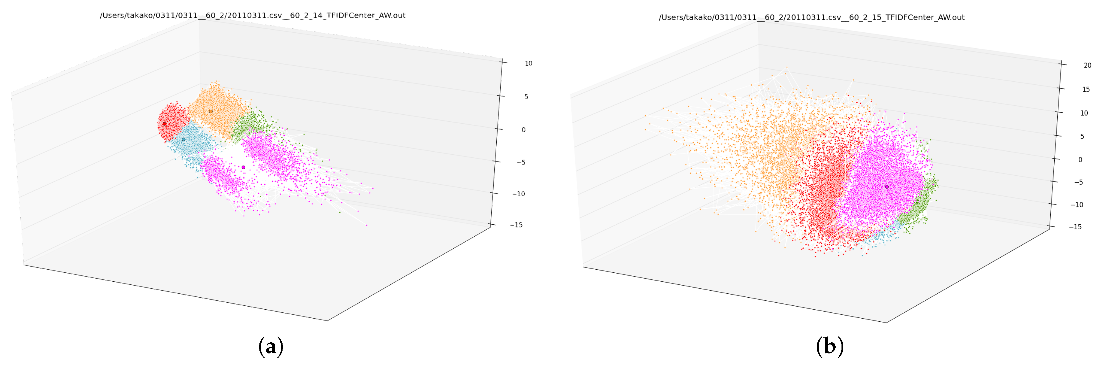
Figure 1 depicts the result of clustering tweets posted to Twitter during two different one-hour windows on the day of the Great East Japan Earthquake, which hit Japan at 2:46 p.m. on 11 March 2011 and inflicted catastrophic damage. Figure 1a plots 97,977 authors who posted 351,491 tweets in total between 2:00 p.m. and 3:00 p.m. on the day of the quake (the quake occurred in the midst of this period of time), while Figure 1b plots 161,853 authors who posted 978,155 tweets between 3:00 p.m. and 4:00 p.m. To plot, we used word-count-based distances between authors and a multidimensional scaling algorithm. Moreover, we grouped the authors into different groups using the k-means clustering algorithm based on the same distances. Dot colors visualize that clustering. We observe a big change in clustering between the hour during which the quake occurred, and the hour after the quake.
Two questions naturally arise: first, what do the clusters mean? Second, what causes the change from Figure 1a to Figure 1b? Answering these questions requires a method for selecting words that best characterize each cluster; in other words, a method for feature selection.
To illustrate, we construct two datasets, one for the timeframe represented in Figure 1a and one for the time-frame represented in Figure 1b, called dataset A and dataset B, respectively. Each dataset consists of a word count vector for each author that reflects all words in all of their tweets. Dataset A has 73,543 unique words, and dataset B has 71,345 unique words, so datasets A and B have 73,543 and 71,345 features, respectively. In addition, each author was given a class label reflecting the category he or she was assigned to from the k-means clustering process.
It was our goal to select a relatively small number of features (words) that were relevant to class labels. We say that a set of features is relevant to class labels, if the values of the features uniquely determine class labels with high likelihood. 
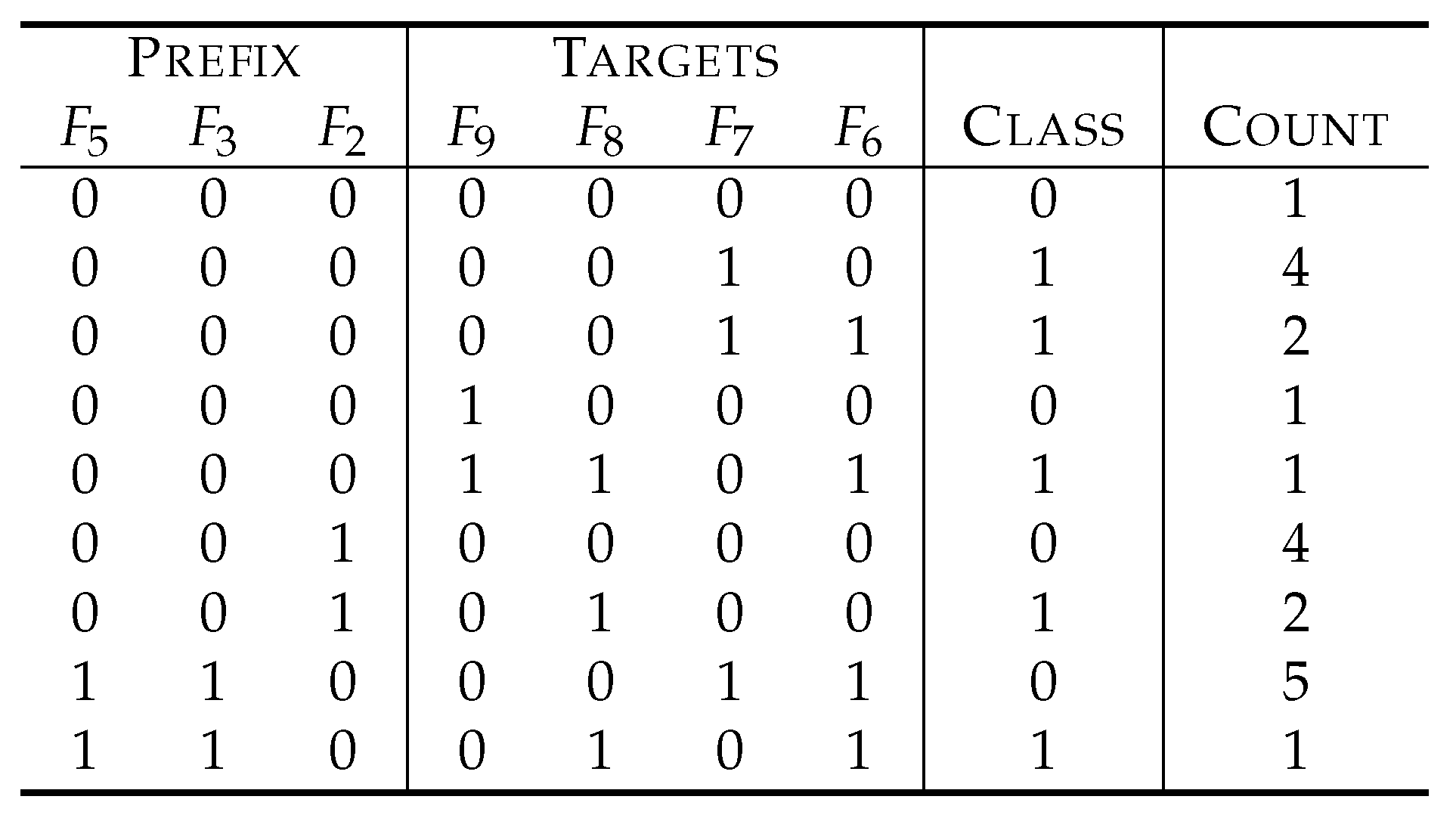
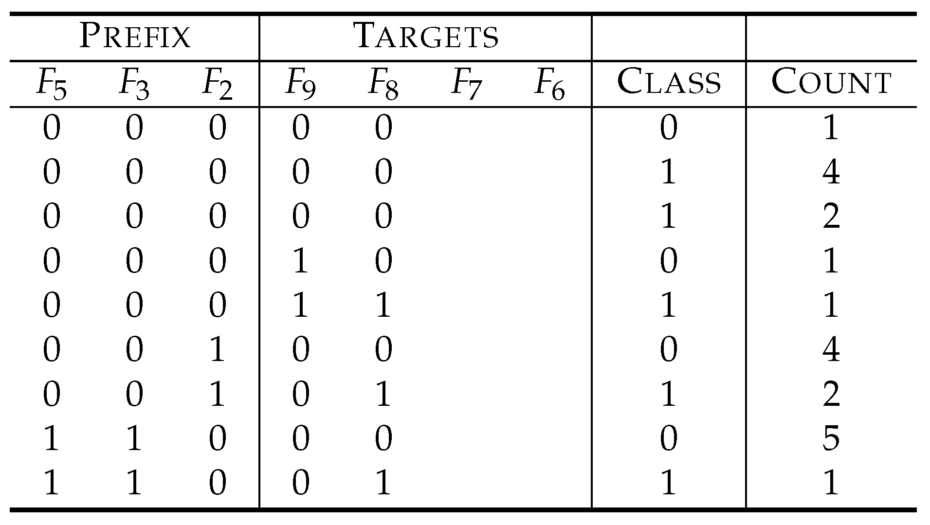
Table 1 depicts an example of a dataset for explanation. F 1 , , F 5 are features, and the symbol C denotes a variable to represent class labels. The feature F 5 , for example, is totally irrelevant to class labels. In fact, we have four instances with F 5 = 0 , and a half of them have the class label 0, while the other half have the class label 1. The same holds true for the case of F 5 = 1 . Therefore, F 5 cannot explain class labels at all and is useless to predict class labels. In fact, predicting class labels based on F 5 has the same success probability as guessing them by tossing a fair coin (the Bayesian risk of F 5 to C is 0.5, which is the theoretical worst). On the other hand, F 1  is more relevant than F 5 because the values of F 1 explain 75% of the class labels, and, in other words, the prediction based on F 1 will be right with a probability of 0.75 (that is, the Bayesian risk is 0.25).
The relevance of individual features can be estimated using statistical measures such as mutual information, symmetrical uncertainty, Bayesian risk and Matthew’s correlation coefficients. For example, at the bottom row of Table 1, the mutual information score I ( F i , C ) of each feature F i to class labels is described. We see that F 1 is more relevant than F 5 , since I ( F 1 , C ) > I ( F 5 , C ) .
To our knowledge, the most common method deployed in big data analysis to select features that characterize class labels is to select features that show higher relevance in some statistical measure. For example, in the example of Table 1, F 1 and F 2 will be selected to explain class labels.
However, when we look into the dataset of Table 1 more closely, we understand that F 1 and F 2 cannot determine class labels uniquely. In fact, we have two instances with F 1 = F 2 = 1 , whose class labels are 0 and 1. On the other hand, F 4 and F 5 as a combination uniquely determine the class labels by the formula of C = F 1 F 2 , where ⊕ denotes the addition modulo two. Therefore, the traditional method based on relevance scores of individual features misses the right answer.
This problem is well known as the problem of feature interaction in feature selection research. Feature selection has been intensively studied in machine learning research. The literature describes a class of feature selection algorithms that can solve this problem, referred to as consistency-based feature selection (for example, [1,2,3,4,5]).
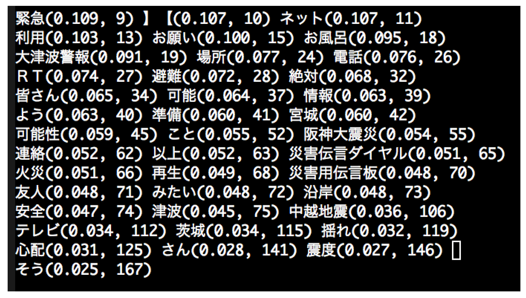
Figure 2 shows the result of feature selection using one of the consistency-based algorithms, namely, Cwc (Combination of Weakest Components) [5]. The dataset used was one generated in the aforementioned way from the tweets of the day when the quake hit Japan and includes 161,425 instances (authors) and 38,822 features (words). The figure shows not only the 40 words selected but also their scores and ranks measured by the symmetrical uncertainty (in parentheses).
This result contains two interesting findings. First, the word ranked 141th is translated as “Mr.”, “Mrs.”, or “Ms.”, which is a polite form of address in Japanese. This form of address is common in Japanese writing, so it seems odd that the word would identify a cluster of authors well. In fact, the relevance of the word is as low as 0.028. However, if we understand the nature of Cwc, we can guess that the word must interact with other features to determine which cluster the author falls inside. In fact, it turns out that the word interacts with the 125th-ranked word, “worry“. Hence, we realize that a portion of those tweets must have been asking about the safety of someone who was not an author’s family member—in other words, someone who the author would have addressed with the polite form of their name.
The second interesting finding is that the words with the highest relevance to class labels have not been selected. For example, the word that means “quake” was ranked at the top but not selected. This is because the word was likely to be used in the tweets with other selected words such as words that translated to “tsunami alert” (ranked 19th), “the Hanshin quake” (55th), “fire” (66th), “tsunami” (75th) and “the Chu-Etsu quake” (106th), so that Cwc judged the word “quake” to be redundant once the co-occurring words had been selected. Our interpretation is that these co-occurring words represent the contexts in which the word “quake” was used, and selecting these words gave us more information than selecting “quake”, which is too general in this case.
Thus, the consistency-based algorithms do not simply select features with higher relevance; instead, they give us knowledge that we cannot obtain from selection based on the relevance of individual features. In spite of these advantages, however, consistency-based feature selection is seldom used in big data analysis. Consistency-based algorithms require heavy computation and the amount of computation increases as the size of data increases so greatly as to make application to large data sets unfeasible.
This paper’s contribution is to improve the run-time performance of two consistency-based algorithms that are known the most accurate, namely Cwc and Lcc (Linear Consistency Constrained feature selection) [4]. We introduce two algorithms that perform well on big data: sCwc and sLcc. They always select the same features as Cwc and Lcc, respectively, and, therefore, perform with the same accuracy. sLcc accepts a threshold parameter to control the number of features to select and has turned out to be as fast as sCwc on average in our experiments.

2. Feature Selection on Categorical Data in Machine Learning Research

In this section, we give a brief review of feature selection research focusing on categorical data. The literature describes three broad approaches: filter, wrapper and embedded. Filter approaches aim to select features based on the intrinsic properties of datasets leveraging statistics and information theory, while wrapper and embedded approaches aim to optimize the performance of particular classification algorithms. We are interested in the filter approach in this paper. We first introduce a legacy feature selection framework and identify two problems in that framework. Then, we introduce the consistency-based approach to solve these problems. For convenience, we will describe a feature or a feature set that is relevant to class labels simply as relevant.

2.1. The Legacy Framework: Sum of Relevance (SR)

In the legacy and fundamental framework of feature selection, which underlies most of the known practical feature selection algorithms, we use sum-of-relevance (SR) functions to evaluate collective relevance of feature sets.
Sum of relevance
Computing the sum of relevance of individual features is an efficient method for estimating the collective relevance.
For example, let I ( F , C ) denote the mutual information of an individual feature F and the class variable C. To be specific, I ( F , C ) is defined by    
I ( F , C ) = x , y Pr [ F = x , C = y ] log Pr [ F = x , C = y ] Pr [ F = x ] Pr [ C = y ] .
The values of x and y are selected from the sample spaces of F and C. It is well known that, the larger I ( F , C ) is, the more tightly F and C correlate with each other. If we do not know the population distribution Pr, we use the empirical distribution derived from a dataset. The sum-of-relevance for a feature set { F 1 , , F n } based on I is determined by
SR ( F 1 , , F n ) = i = 1 n I ( F i , C ) ,
and estimates the collective relevance of { F 1 , , F n } .
The principle of SR-based feature selection is to find a good balance to the trade-off between the SR value of and the number of features to select. This can be achieved efficiently by computing the relevance of individual features and sorting the features with respect to the computed relevance scores. For example, Table 1 shows a dataset, and we see the relevance of each feature measured by the mutual information at the bottom row. Since I ( F 1 , C ) = I ( F 2 , C ) 0.13 , I ( F 3 , C ) 0.03 and I ( F 4 , C ) = I ( F 5 , C ) = 0 hold, if the requirement is to select two features that maximize the SR value, the best choice is definitely F 1 and F 2 . If the requirement is to select the smallest feature set whose SR value is no smaller than 0.25, the answer should be F 1 and F 2 as well. As a substitute for mutual information, we can use the Bayesian risk, the symmetrical uncertainty and Matthews correlation coefficients, for example.
Relief-F [6] is a well-known example of a feature selection algorithm that relies only on SR functions. For the underlying relevance function, Relief-F uses a distance-based randomized function. Since computing this distance-based relevance function requires relatively heavy computation, Relief-F is not very fast, but, in general, the simple SR-based feature selection scales and can be applied to high-dimensional data.

2.2. The Problem of Redundancy

The simple SR-based feature selection has, however, two important problems that will harm the collective relevance of selected features. One of them is the problem caused by internal correlation, which is also known as the problem of redundancy. The problem is described as follows.
Problem of redundancy
Feature selection by SR may select features that are highly mutually correlated, and such high internal correlation definitely decreases the collective relevance of the features.
The dataset of Table 2 is obtained by adding the feature F 6 to the dataset of Table 1. Eventually, F 6  is a copy of F 1 , and, hence, I ( F 6 , C ) = I ( F 1 , C ) 1.3 holds. To select two features that maximize the SR value, we have three answer candidates this time, that is, { F 1 , F 2 } , { F 1 , F 6 } and { F 2 , F 6 } . Among the candidates, { F 1 , F 6 } is clearly a wrong answer, since its joint relevance has no gain over the individual relevance of F 1 and F 6 .
This thought experiment inspires us to pay attention to the internal correlation among features. If the internal correlation among features is greater, the features include more redundancy when they determine classes. For example, if we use mutual information to evaluate internal correlation, the internal correlation of { F 1 , F 2 } is computed to be I ( F 1 , F 2 ) = 0 , that is, F 1 and F 2 are independent of each other. On the other hand, the internal correlation of { F 1 , F 6 } is I ( F 1 , F 6 ) = H ( F 1 ) 0.68 . Therefore, the set of { F 1 , F 6 } includes more redundancy than { F 1 , F 2 } , and, hence, we should select { F 1 , F 2 } rather than { F 1 , F 6 } . The principle of minimizing redundancy (MR) is to design feature selection algorithms so that they avoid selecting features that have high internal correlation.
The algorithm of mRMR (Minimum Redundancy and Maximum Relevance) [7] is a well-known greedy forward selection algorithm that maximizes the sum of relevance (SR) with respect to the mutual information and minimizes the internal redundancy determined by
IC ( F 1 , , F n ) = 1 n 2 i = 1 n j = 1 n I ( F i , F j ) .
Fcbf (Fast Correlation-Based Filter) [8] and Cfs (Correlation-based Feature Selection) [9] are also known to be based on the principle of minimizing redundancy.
Although the principle of minimizing redundancy definitely improves the actual collective relevance of features to select, it cannot solve the other problem of the SR framework, which we state next.

2.3. The Problem of Feature Interaction

We start with describing the problem.
Problem of feature interaction
Feature selection by SR may miss features if their individual relevance is low but they show high collective relevance by interacting one another.
For the datasets of Table 1 and Table 2, F 4 and F 5 determine the class C by the formula of C = F 4 F 5 , where ⊕ denotes the addition modulo two, and, hence, their collective relevance is the highest. Nevertheless, the sum of relevance for { F 4 , F 5 } is zero, and, hence, the feature selection algorithms that we saw in Section 2.1 and Section 2.2 have no chance to select { F 4 , F 5 } .
This problem is explained by interaction among features: when more than one features that individually show only low relevance exhibit high collective relevance, we say that the features interact with each other. As shown in the example above, neither the SR principle nor the MR principle can incorporate feature interaction into the results of feature selection.
The literature provides two approaches to solve this problem: rule-based, and consistency-based. We will define these approaches here.
Frfs (FOIL Rule based Feature subset Selection) [10] is a characteristic example of a rule-based feature selection algorithm. The algorithm first extracts events of feature interaction from a dataset as frequent rules. Each rule is in the form of ( f 1 , , f k ) c such that the antecedent f 1 , , f k are feature values and the consequent c is a class label. Frfs can perform the rule extraction efficiently by leveraging First Order Inductive Learner (FOIL) [11]. However, it is still too slow to apply to big data analysis.

2.4. Consistency-Based Feature Selection

The consistency-based approach solves the problem of feature interaction by leveraging consistency measures. A consistency measure is a function that takes sets of features as input rather than individual features. Furthermore, a consistency measure is a function that represents collective irrelevance of the feature set input, and, hence, the smaller a value of a consistency measure is, the more relevant the input feature set is.
Moreover, a consistency measure is required to have the determinacy property: its measurement is zero, if, and only if, the input feature set uniquely determines classes.
Definition 1.
A feature set of a dataset is consistent, if, and only if, it uniquely determines classes, that is, any two instances of the dataset that are identical with respective to the values of the features of the feature set have the identical class label as well.
Hence, a consistency measure function returns the value zero, if, and only if, its input is a consistent feature set. An important example of the consistency measure is the Bayesian risk, also known as the inconsistency rate [2]:
Br ( F 1 , , F n ) = 1 x 1 , , x n max y Pr [ F 1 = x 1 , , F n = x n , C = y ] .
The variable x i moves in the sample space of F i , while the variable y moves in the sample space of C. It is evident that the Bayesian risk is non-negative, and determinacy follows from
x 1 , , x n max y Pr [ F 1 = x 1 , , F n = x n , C = y ] x 1 , , x n Pr [ F 1 = x 1 , , F n = x n ] = 1 .
Another important example of the consistency measure is the binary consistency measure, defined as follows:
Bn ( F 1 , , F n ) = 0 , if { F 1 , , F n } is consistent ; 1 , otherwise .
Focus [1], the first consistency-based algorithms in the literature, performs an exhaustive search to find the smallest feature set { F 1 , , F n } with Bn ( F 1 , , F n ) = 0 .
Apparently, Focus cannot be practically fast. In general, consistency-based feature selection has problems in time-efficiency because of the broadness of the search space. In fact, the search space should be the power set of the entire set of features, and its size is an exponential function of the number of features.
Problem of consistency measures
When N features describe a dataset, the number of the possible input to a consistency measure is as large as 2 N .
The monotonicity property of consistency measures helps to solve this problem. The Bayesian risk, for example, has this property: if F G , Br ( F ) Br ( G ) holds, where F and G are feature subsets of a dataset. Almost all of the known consistency measures such as the binary consistency measure and the conditional entropy H ( C F ) = H ( C ) I ( F , C ) have this property as well. In [5], the consistency measure is formally defined as a non-negative function that has the determinacy and monotonicity properties.
Although some of the algorithms in the literature such as Abb (Automatic Branch and Bound) [2] took advantage of the monotonicity property to narrow their search space, the real breakthrough was yielded by Zhao and Liu in their algorithm Interact [3]. Interact uses the combination of the sum-of-relevance function based on the symmetrical uncertainty and the Bayesian risk. The symmetrical uncertainty is a harmonic mean of the ratios of I ( F , C ) / H ( F ) and I ( F , C ) / H ( C ) and hence turns out to be
SU ( F ; C ) = 2 I ( F , C ) H ( F ) + H ( C ) .
The basic idea of Interact is to narrow down the search space boldly and to take SR values of the symmetrical uncertainty into account to cover the caused decrease of relevance. Although the search space of Interact is very narrow, the combination of the SR function and the consistency measure keeps the accuracy performance good. Lcc [4] improves Interact and can exhibit better accuracy. Although Interact and Lcc are much faster than previous consistency-based algorithms described in the literature, they are not fast enough to apply to large datasets with thousands of instances and features.
Cwc [5] is a further improvement and replaces the Bayesian risk with the binary consistency measure, which can be computed faster. Cwc is reported to be about 50 times faster than Interact and Lcc on average. In fact, Cwc performs feature selection for a dataset with 800 instances and 100,000 features in 544 s, while Lcc does it in 13,906 s. Although the improvement was remarkable, Cwc is not fast enough to apply to big data analysis.

2.5. Summary

Figure 3 summarizes the progress of feature selection in the literature. The legacy framework of sum-of-relevance (SR) has the problems of redundancy and feature interaction. The principle of minimizing redundancy (MR) in combination with SR solves the problem of redundancy and provides practical algorithms such as mRMR. Furthermore, using consistency measures (CM) solves the problem of feature interaction, but is time-consuming because complete (exhaustive) search (CS) is necessary. On the other hand, the combination of SR and CM allows linear search (LS) and improves the low time-efficiency of the consistency-based feature selection dramatically. In particular, Cwc is the fastest and the most accurate consistency-based algorithm and is comparable with Frfs, which is rule-based. Nevertheless, Cwc or Frfs does not scale well for big data analysis.

3. sCwc and sLcc

sCwc and sLcc improve the time efficiency of Cwc and Lcc significantly. The letter “s” of sCwc and sLcc represents “scalable”, “swift” and “superb”.

3.1. The Algorithms

We start by explaining the Cwc algorithm. Figure 1 depicts the algorithm. Given a dataset described by a feature set { F 1 , , F N } , Cwc aims to output a minimal consistent subset S { F 1 , , F N } .
Definition 2.
A minimal consistent subset S satisfies Bn ( S ) = 0 and Bn ( T ) > 0 for any proper subset T S .
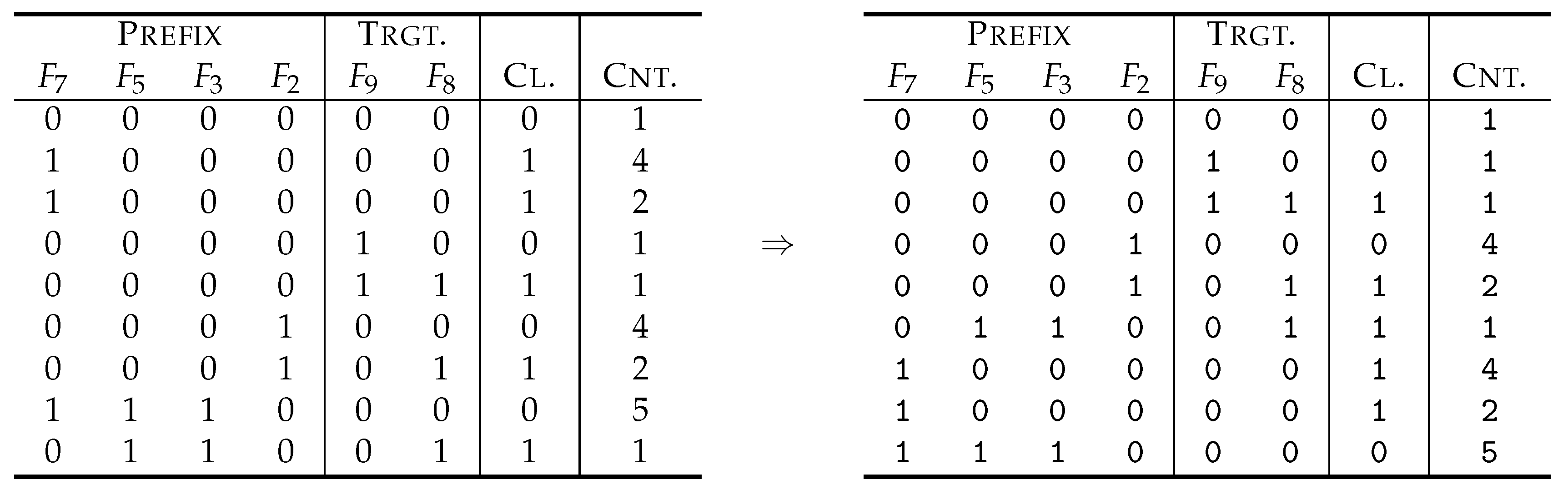
Achieving this goal is, however, impossible if Bn ( F 1 , , F N ) > 0 holds, since Bn ( S ) Bn ( F 1 , , F N ) > 0 always holds by the monotonicity property of Bn . Therefore, the preliminary step of Cwc is to remove the cause of Bn ( F 1 , , F N ) > 0 . To be specific, if Bn ( F 1 , , F N ) > 0 , there exists at least one inconsistent pair of instances, which are identical with respect to the feature values but with different class labels. The process of denoising is thus to modify the original dataset so that it includes no inconsistent pairs. To denoise, we have two approaches as follows:
  • We can add a dummy feature F ^ to { F 1 , , F N } and can assign a value of F ^ to an instance so that, if the instance is not included in any inconsistent pair, the assigned value is zero; otherwise, the assigned value is determined depending on the class label of the instance.
  • We can eliminate at least a part of the instances that are included in inconsistent pairs.
Although both of the approaches can result in Bn ( F 1 , , F N ) = 0 , the former seems better because useful information may be lost by eliminating instances. Fortunately, high-dimensional data usually have the property of Bn ( F 1 , , F N ) = 0 from the beginning since N is very large. When Bn ( F 1 , , F N ) = 0 , denoising is benign and does nothing.
On the other hand, to incorporate sum-of-relevance into consistency-based feature selection, we sort features in the incremental order of their symmetrical uncertainty scores, that is, we renumber F i s so that SU ( F i ) SU ( F j ) if i < j . The symmetrical uncertainty, however, is not the mandatory choice, and we can use any measure to evaluate relevance of an individual feature so that, the greater a value of the measure is, the more relevant the feature is. For example, we can replace the symmetrical uncertainty with the mutual information I ( F , C ) .
Cwc deploys a backward elimination approach: it first sets a variable S to the entire set { F 1 , , F N } and then investigates whether each F i can be eliminated from S without violating the condition of Bn ( S ) = 0 . That is, S is updated by S = S { F i } , if, and only if, Bn ( S { F i } ) = 0 . Hence, Cwc continues to eliminate features until S becomes a minimal consistent subset. Algorithm 1 describes the algorithm of Cwc.
The order of investigating F i is the incremental order of i, and, hence, the incremental order of SU ( F i ) . Since F i is more likely to be eliminated than F j with i < j , we see that Cwc stochastically outputs minimal consistent subsets with higher sum-of-relevance scores.
Algorithm 1 The algorithm of Cwc [5]
Require: A dataset described by { F 1 , , F N } with Bn ( F 1 , , F N ) = 0 .
Ensure: A minimal consistent subset S { F 1 , , F N } .
1:
Sort F 1 , , F N in the incremental order of SU ( F i ; C ) .
2:
Let S = { F 1 , , F N } .
3:
for i = 1 , , N do
4:
    if Bn ( S { F i } ) = 0 then
5:
        update S by S = S { F i } .
6:
    end if
7:
end for
To improve the time efficiency of Cwc, we restate the algorithm of Cwc as follows. To illustrate, let S 0 be a snapshot of S immediately after Cwc has selected F k . In the next step, Cwc investigates whether Bn ( S 0 { F k + 1 } ) = 0 holds. If so, Cwc investigates whether Bn ( S 0 { F k + 1 , F k + 2 } ) = 0 holds. Cwc continues the same procedure, until it finds F with Bn ( S 0 { F k + 1 , F k + 2 , , F } ) > 0 . This time, Cwc does not eliminate F . S is set to S 0 { F k + 1 , F k + 2 , , F 1 } , and Cwc investigate F + 1 next. Thus, to find F to be selected, Cwc solves the problem to find such that
= min { i i { k + 1 , , N } , Bn ( S { F k + 1 , , F i } ) > 0 } .
To solve the problem, Cwc relies on linear search.
On the other hand, the idea of improving Cwc is obtained by looking at the same problem from a different direction. By the monotonicity property of Bn, Bn ( S 0 { F k + 1 , F k + 2 , , F i } ) Bn ( S 0 { F k + 1 , F k + 2 , , F } ) > 0 holds for any i , and, therefore, the formula
1 = max { i i { k + 1 , , N } , Bn ( S { F k + 1 , , F i } ) = 0 }
also characterizes .
This characterization of indicates that we can take advantage of binary search instead of linear search to find (Algorithm 2). Since the average time complexity of the binary search is O ( log ( N k ) ) , we can expect significant improvement compared with the time complexity of O ( N k ) of the linear search used in Cwc. Algorithm 3 depicts our improved algorithm, sCwc.
Algorithm 2 Binary search to find
Require: S { F 1 , , F N } and k { 1 , , N 1 } such that S { F k , , F N } and Bn ( S ) = 0 .
Ensure: { k + 1 , , N } such that = arg min { Bn ( S { F k + 1 , , F i } ) > 0 i = k + 1 , , N } .
1:if Bn ( S { F k + 1 , , F N } ) = 0 then
2:     = None . ▹ No such exists.
3:else
4:    Let l o w , h i g h , m i d = k , N , l o w + h i g h 2 .
5:    repeat
6:        if Bn ( S { F k + 1 , , F m i d ) > 0 then
7:           Let h i g h = m i d .
8:        else
9:           Let l o w = m i d .
10:        end if
11:        Let m i d = l o w + h i g h 2 .
12:    until m i d = h i g h holds.
13:     = h i g h .
14:end if
In addition, Algorithm 4 depicts the algorithm of Lcc [4]. In contrast to Cwc, Lcc accepts a threshold parameter δ 0 . The parameter determines the strictness of its elimination criteria. The greater δ is, the looser the criteria is, and, therefore, the smaller features Lcc selects.
There are two major differences between Lcc and Cwc: first, Lcc does not require that the entire feature set { F 1 , , F N } is consistent. Therefore, denoization to make Bn ( F 1 , , F N ) = 0 is not necessary. Secondly, the elimination criteria of Bn ( S { F i } ) = 0 of Cwc is replaced with Br ( S { F i } ) δ . By the determinacy property, Br ( S { F i } ) = 0 , if, and only if, Bn ( S { F i } ) = 0 . Hence, with δ = Br ( F 1 , , F N ) = 0 , Lcc selects the same features as Cwc does.
Algorithm 3 The algorithm of sCwc
Require: A dataset described by { F 1 , , F N } with Bn ( F 1 , , F N ) = 0 .
Ensure: A minimal consistent subset S { F 1 , , F N } .
1:Sort F 1 , , F N in the incremental order of SU ( F i ; C ) .
2:Let S = { F 1 , , F N } .
3:Let k = 0 .
4:repeat
5:    Find = arg min { Bn ( S { F k + 1 , , F i } ) > 0 i = k + 1 , , N } by binary search.
6:    if does not exist then
7:        Let = N + 1 .
8:    end if
9:    Update S by S = S { F k + 1 F 1 } .
10:    Let k = .
11:until k N holds.
Algorithm 4 The algorithm of Lcc  [4]
Require: A dataset described by { F 1 , , F N } and a non-negative threshold δ .
Ensure: A minimal δ -consistent subset S { F 1 , , F N } .
1:
Sort F 1 , , F N in the incremental order of SU ( F i ; C ) .
2:
Let S = { F 1 , , F N } .
3:
for i = 1 , , N do
4:
    if Br ( S { F i } ) δ then
5:
        update S by S = S { F i } .
6:
    end if
7:
end for
Since the Bayesian risk has the monotonicity property as well, b i = Br ( S { F k + 1 , , F i } ) compose an increasing progression, and, hence, we can find such that
= min { i i { k + 1 , , N } , Br ( S { F k + 1 , , F i } ) > δ } = 1 + max { i i { k + 1 , , N } , Br ( S { F k + 1 , , F i } ) δ }
very efficiently by means of binary search. Algorithm 5 describes the improved algorithm of sLcc based on binary search.
Algorithm 5 The algorithm of sLcc
Require: A finite dataset and a non-negative threshold δ .
Ensure: A minimal δ -consistent subset S { F 1 , , F N } .
1:Sort F 1 , , F N in the incremental order of SU ( F i ; C ) .
2:Let S = { F 1 , , F N } .
3:Let k = 0 .
4:repeat
5:    Find = arg min { Br ( S { F k + 1 , , F i } ) > δ i = k + 1 , , N } by binary search.
6:    if does not exist then
7:        Let = N + 1 .
8:    end if
9:    Update S by S = S { F k + 1 F 1 } . Let k = .
10:until k N holds.

3.2. Complexity Analysis

When N F and N I denote the number of features and instances of a dataset, the average time complexity of Cwc is estimated by O ( N F N I ( N F + log N I ) ) [12]. The first term O ( N F 2 N I ) represents the feature selection computation, while the second term O ( N F N I log N I ) shows the instance sorting process. In [12], it is shown that sorting instances at the initial stage of the algorithm is highly effective for investigating Bn ( S { F i } ) = 0 efficiently (see also Section 6.1). Since sCwc improves the time-efficiency of selecting features by replacing the linear search of Cwc with binary search, we can estimate its time complexity by O ( N F N I ( log N F + log N I ) ) . By the same analysis, we can conclude that the same estimate of time complexity applies to sLcc.
We have verified this estimate of time complexity through experiments using high-dimensional datasets described in Table 3, whose dimensions vary from 15,741 to 38,822. Figure 4 plots the experimental results: the x-axis represents N F N I ( log N F + log N I ) , while the y-axis represents run-time of sCwc in milliseconds. We observe that the plots are approximately aligned along a straight line, and, hence, can conclude that the aforementioned estimate is right.

4. Comparison of Feature Selection Algorithms

We compare sCwc and sLcc with four benchmark algorithms, namely, Frfs, Cfs, Relief-F and Fcbf, with respect to the accuracy, the run-time and the number of features selected. Frfs [10] is a rule-based algorithm, while Cfs [9], Relief-F [13] and Fcbf [8] are sum-of-relevance-based algorithms. In addition, Cfs and Relief-F are designed to avoid redundant selection of features.

4.1. Datasets to Use

For the comparison, we use 15 relatively large datasets, since the benchmark algorithms are not fast enough to apply to really high-dimensional datasets such as those described in Table 3. Table 4 describes the datasets, and Figure 5 plots the number of features N F (x-axis) and the number of instances N I (y-axis) of each dataset.
To make the comparison fair, ten of the datasets are chosen from the feature selection challenges of Neural Information Processing Systems (NIPS) 2003 [14] and World Congress on Computational Intelligence (WCCI) 2006 [15]. The datasets of NIPS 2003 emphasize the largeness of the feature number N F , while those of WCCI 2006 do the instance number N I . The remaining five datasets are retrieved from the University of California, Irvine (UCI) repository of machine learning databases [16].

4.2. Comparison of Accuracy

When the input dataset is described by a consistent feature set, that is, when Bn ( { F 1 , , F N } ) = 0 holds, sLcc with δ = 0 selects the same features as sCwc does. Hence, we compare the best the area under an receiver operating characteristic curve (AUC-ROC) scores of sLcc when the parameter δ varies from 0 to 0.02 at interval of 0.002 with the AUC-ROC scores of the other benchmark algorithms. In addition, since many of the benchmark algorithms cannot finish feature selection for the dataset Dorothea within a reasonable time allowance, we do not use the dataset for the purpose of comparison in accuracy.

4.2.1. Method

We generate 10 pairs of training and test data subsets from each dataset of Figure 5 by distributing the instances to test and training data subsets at random with a ratio of 4:1, and perform the following for each pair:
(1)
We run the feature selection algorithms on the training data subset and then reduce the training dataset so that the selected features describe the reduced training data subset.
(2)
We reduce the test data subset so that the selected features describe the reduced test data subset.
(3)
We train three classifiers with the reduced training data subset. The classifiers to use are C Support Vector Machine with Radial Base Function (RBF-Kernel-C-SVM), Naïve Bayes and C4.5. Optimal values for the γ and C parameters of the RBF-kernel-C-SVM and the confidence factor of C4.5 are chosen through grid search with ten-fold cross validation on the reduced training data subset.
(4)
We make the trained classifiers predict class labels for all of the instances of the reduced test data subset and compute scores of the accuracy measures of AUC-ROC (Area Under Curve of ROC curve) and F-measure by comparing the obtained prediction and the true class labels.
For sLcc, we run experiments with sLcc changing δ from 0 to 0.02 at interval of 0.002 and select the best scores.

4.2.2. Results and Analysis

Table 5, Table 6, Table 7, Table 8, Table 9 and Table 10 describe the result of the comparison. For each combination of a classifier and an accuracy measure, we see the raw scores of the six feature selection algorithms in the upper rows and their rankings in the lower rows. Figure 6 and Figure 7 also depict the same information, where sLcc, Frfs, Cfs, Relief-F and Fcbf are displayed in the colors of blue, orange, gray, yellow and light blue, respectively.
Remarkably, for all the combinations of classifiers and accuracy measures, sLcc and Frfs monopolize the first and second places with respect to both of the averaged raw scores and ranks. Furthermore, sLcc outperforms the others except for the combination of Naïve Bayes and AUC-ROC with respect to the averaged raw scores. With respect to the averaged ranks, sLcc is ranked top for the combinations of SVM and AUC-ROC, SVM and F-Score and Naïve Bayes and F-Score, while Frfs outperforms sLcc for the other three combinations.
Table 11 shows for each feature selection algorithm its averaged scores of AUC-ROC score and F-measure across the three classifiers and the 15 datasets. We see that sLcc outperforms the other algorithms for both AUC-ROC and F-Scores. Table 11 also shows the averaged ranks of the feature selection algorithms across the two accuracy measures, three classifiers and the 14 datasets. sLcc and Frfs turn out to have the same averaged rank, and they are evidently superior to the other three benchmark algorithms.
To verify the observed superiority of sLcc and Frfs, we conduct non-parametric multiple comparison tests following the recommendation by Demšar [17]. To be specific, we have performed the Friedman test and then the Hommel test. To avoid the type II error of a multiple comparison test, the tests are conducted only once based on the averaged ranks displayed in Table 11, which are computed across all of the combinations of a classifier, an accuracy measures and a dataset. The results of the tests are described in the left column of Table 11. For the Freedman test, the observed p-value is extremely small and displayed as 0.00, and, therefore, we reject the null hypothesis and conclude that there exists a statistically significant difference among the feature selection algorithms. In the Hommel test, which follows the Friedman test, we use sLcc as a control. The calculated p-values are negligibly small for Cfs, Relief-F and Fcbf, and, hence, we can conclude that the observed superiority of sLcc to Cfs, Relief-F and Fcbf is statistically significant. On the other hand, the results of the Hommel test indicates that sLcc and Frfs are compatible with each other, since the corresponding p-value is as great as 0.981, which is very close to 1.0.
As a conclusion, to obtain high accuracy, we can recommend to use sLcc and Frfs for feature selection. To emphasize the difference between these two algorithms, sLcc will perform better when used with SVM, while Frfs will perform better when used with C4.5.

4.2.3. Accuracy of sLcc for Various δ

Figure 8 shows the results of experiments of performing sLcc changing the value of δ from 0 to 0.02 at interval of 0002: the AUC-ROC scores computed based on the results when using the RBF-kernel-C-SVM as a classifier for different values of δ are displayed in orange per dataset.
For the seven datasets of Gina, Gisette, Hiva, Mushroom, Nova and Silva, that is, for almost half of the datasets investigated, the AUC-ROC score reaches the maximum when δ = 0 . On the other hand, we should note that the results for Kr-vs-Kp and Madelon show steep drop-offs of the AUC-ROC score at δ = 0 . Since sLcc outputs the same results as sCwc does in most of cases when δ = 0 , these results imply a clever way to use sCwc and sLcc: we can try sCwc first and then apply sLcc if good results are not obtained from sCwc.
Figure 8 also includes plots of the numbers of features selected (plots and lines in blue). In theory, running sLcc with a greater δ will results in selection of a smaller number of features. The results of the experiments support this only except for Gina.

4.3. Time-Efficiency

Table 12 describes the experimental results of the run-time performance of sLcc, sCwc, Frfs, Cfs, Relief-F, Fcbf, Lcc, Cwc and Interact. The feature selection algorithm of Interact was not used for the comparison in accuracy, since it was shown in [12] that Lcc always outperform Interact with respect to accuracy. In the experiment, we use six datasets out of the 15 datasets described in Table 4. These six datasets need a relatively long time to perform feature selection and are appropriate for the purpose of comparing the time-efficiency of feature selection algorithms. Furthermore, we use a Mac Book Pro (2016, Apple Inc., Cupertino, CA, USA) with Quad Core i7 2.5 GHz processor and 8 GB memory. The threshold parameter δ for sLcc and Lcc is set to 0.01.
From the result, we see that sLcc and sCwc outperform the others, and they have greatly improved the performance of Cwc and Lcc. In particular, the extent of the improvement of sLcc from Lcc is remarkably greater than that of sCwc from Cwc. In fact, from Table 12, we see that, even though there is a significant difference in run-time between Lcc and Cwc, the run-time performance of sLcc and sCwc appears comparable with each other. This can be explained as follows: with a greater δ , sLcc/Lcc eliminates more features; in other words, the intervals between adjacent selected features become wider; this implies that the number of features investigated by binary search decreases, while the number of features investigated by linear search remains the same; thus, as δ increases, the extent of improvement by sLcc over Lcc becomes more significant.
The experimental results depicted by Figure 9 supports this discussion. Since Lcc relies on linear search, every feature is evaluated exactly one time regardless of the value of δ . Hence, the run-time of Lcc remains the same even if δ changes. By contrast, as Figure 9 shows, the run-time of sLcc decreases as δ increases. This is because the number of features selected decreases as δ increases, and, consequently, sLcc investigates a fewer number of features. When looking at Figure 8 from this viewpoint, we realize that it is a basic tendency that the number of features selected is a decreasing function of δ (the dataset of Gina is the only exception).
Table 12 also shows the results of the Hommel test to compare sLcc with Frfs, Cwc and Interact, selected from the feature selection algorithms that can finish feature selection within a reasonable time allowance for all of the six datasets: Frfs is the fastest of the benchmark algorithms; Cwc is included to show the degree of improvement by sLcc; Interact is included because it is well known as the first consistency-based feature selection algorithm that is practically efficient. The displayed p-values indicate that the observed superiority of sLcc is statistically significant for the significance level of 5 % . These datasets are, however, significantly smaller in size than the data to which we intend to apply sLcc and sCwc. We further investigate the efficiency performance of sLcc and sCwc in the next section.

5. Performance of sLcc and sCwc for High-Dimensional Data

In this section, we look into both of the accuracy and time-efficiency performance of sLcc and sCwc when applied to high-dimensional data. We use 26 real datasets studied in social network analysis, which were described in Section 1 as well. These datasets were generated from the large volume of tweets sent to Twitter on the day of the Great East Japan Earthquake, which hit Japan at 2:46 p.m. on 11 March 2011 and inflicted catastrophic damage. Each dataset was generated from a collection of tweets posted during a particular time window of an hour in length and consists of a word count vector for each author of Twitter that reflects all words in all they sent during that time window. In addition, each author was given a class label reflecting the category he or she was assigned from the k-means clustering process. We expect that this annotation represents the extent to which authors are related to the Great East Japan Earthquake.
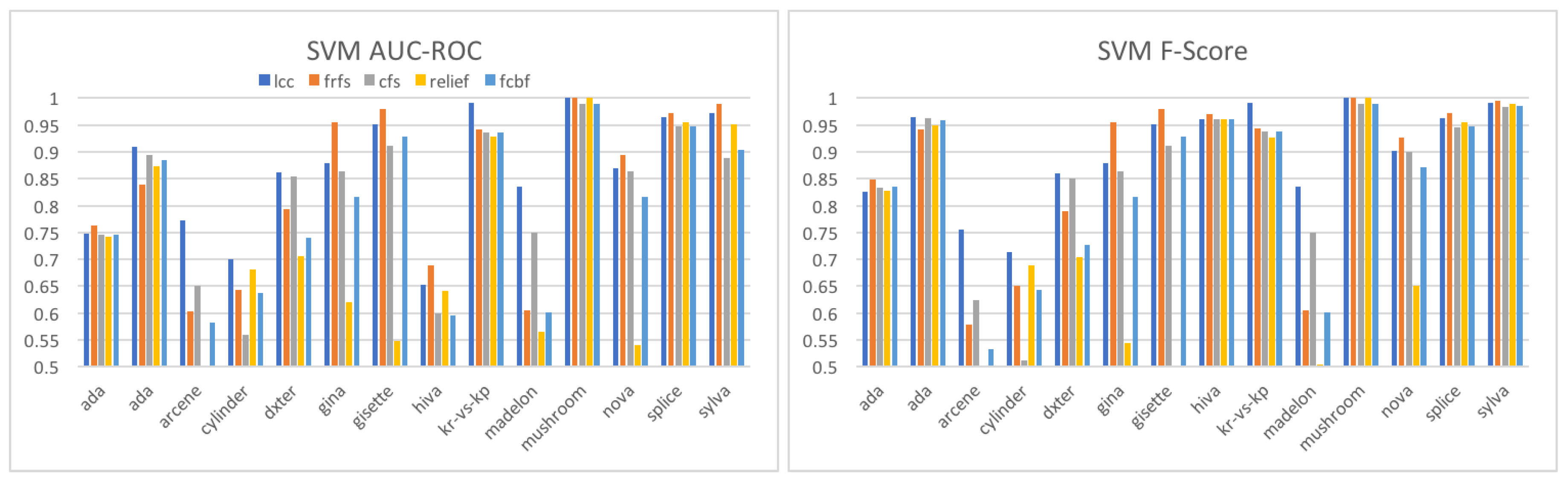
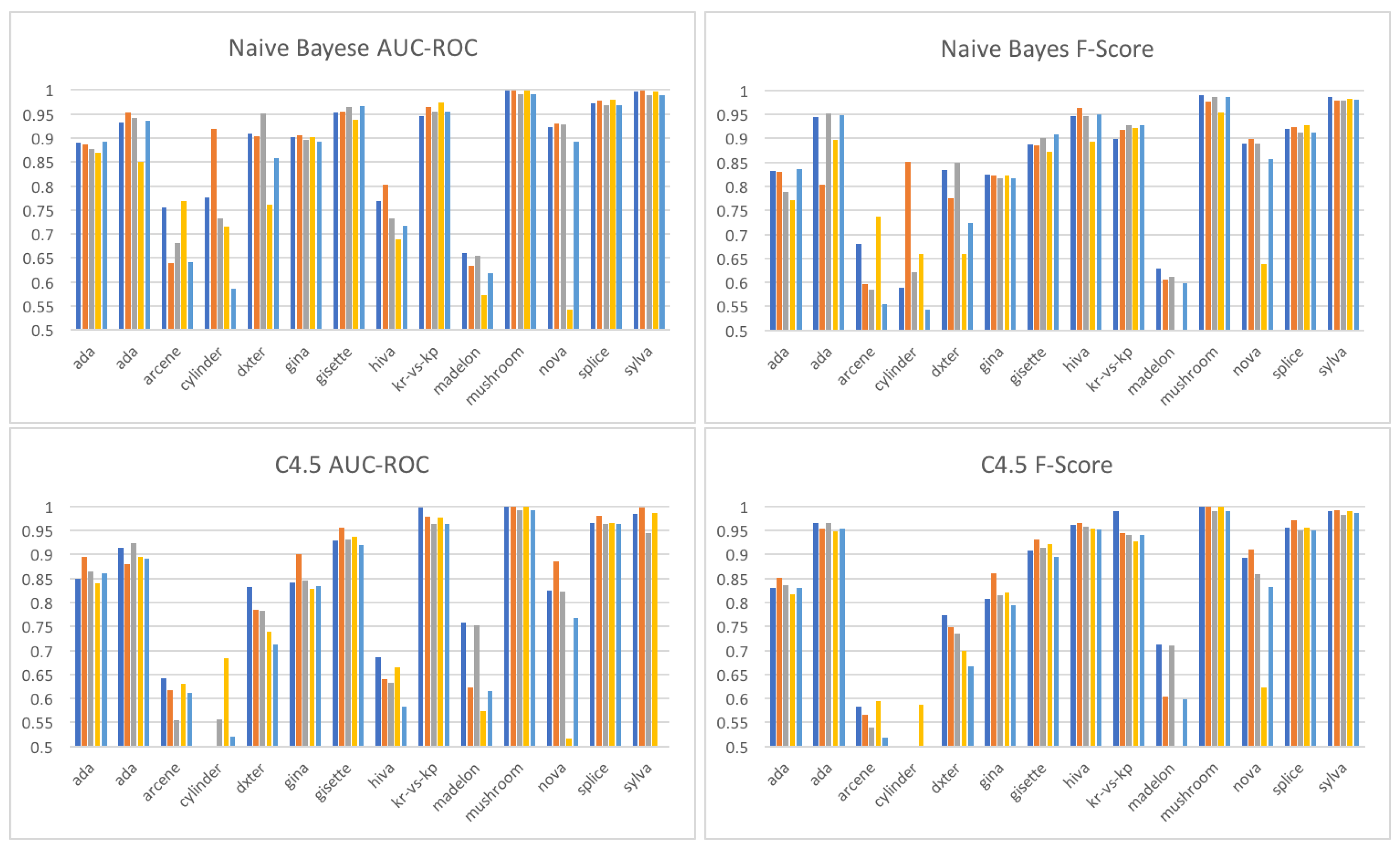
Table 13 shows the AUC-ROC scores of C-SVM that run on the features selected by sCwc. We measured the scores using the method described in Section 4.2.1. Given time constraints, we use only 18 datasets out of the 26 datasets prepared. We see that the scores are significantly high, and the features selected well characterize the classes.
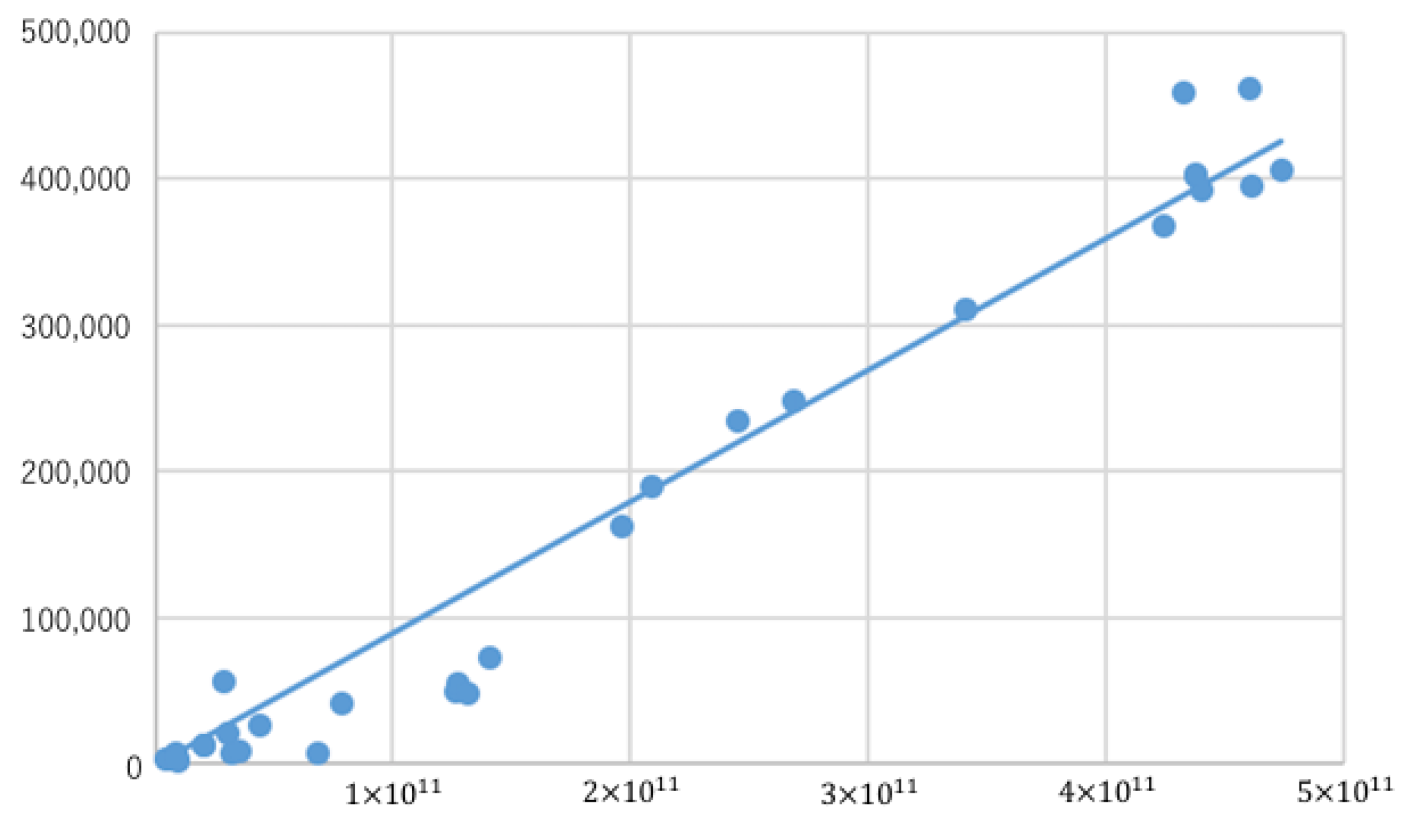
From Table 3, we observe that the run-times of sCwc on the aforementioned 26 datasets range from 1.397 s to 461.130 s, and the average is 170.017 s. Thus, this experiment shows that the time-efficiency of sCwc is satisfactory enough to apply it to high-dimensional data analysis.
For a more precise measurement, we compare sCwc with Frfs. Table 14 shows the results. Since running Frfs takes much longer, we test only three datasets and use a more powerful computer with CentOS release 5.11 (The CentOS Project), Intel Xeon X5690 6-Cores 3.47 GHz processor and 192 GB memory (Santa Clara, CA, USA). Although we tested only a few datasets, the superiority of sCwc to Frfs is evident: sCwc is more than twenty times faster than Frfs.
In addition, we can conclude that sCwc remarkably improves the time-efficiency of Cwc. Running Cwc on the smallest dataset with 15,567 instances and 15,741 features in Table 3 requires several hours to finish feature selection. Based on this, we estimate that it will take up to ten days to process the largest dataset with 200,569 instances and 99,672 features because we know the time complexity of Cwc is O ( N F N I ( N F + log N I ) ) . Surprisingly, sCwc has finished feature selection of this dataset in only 405 s.
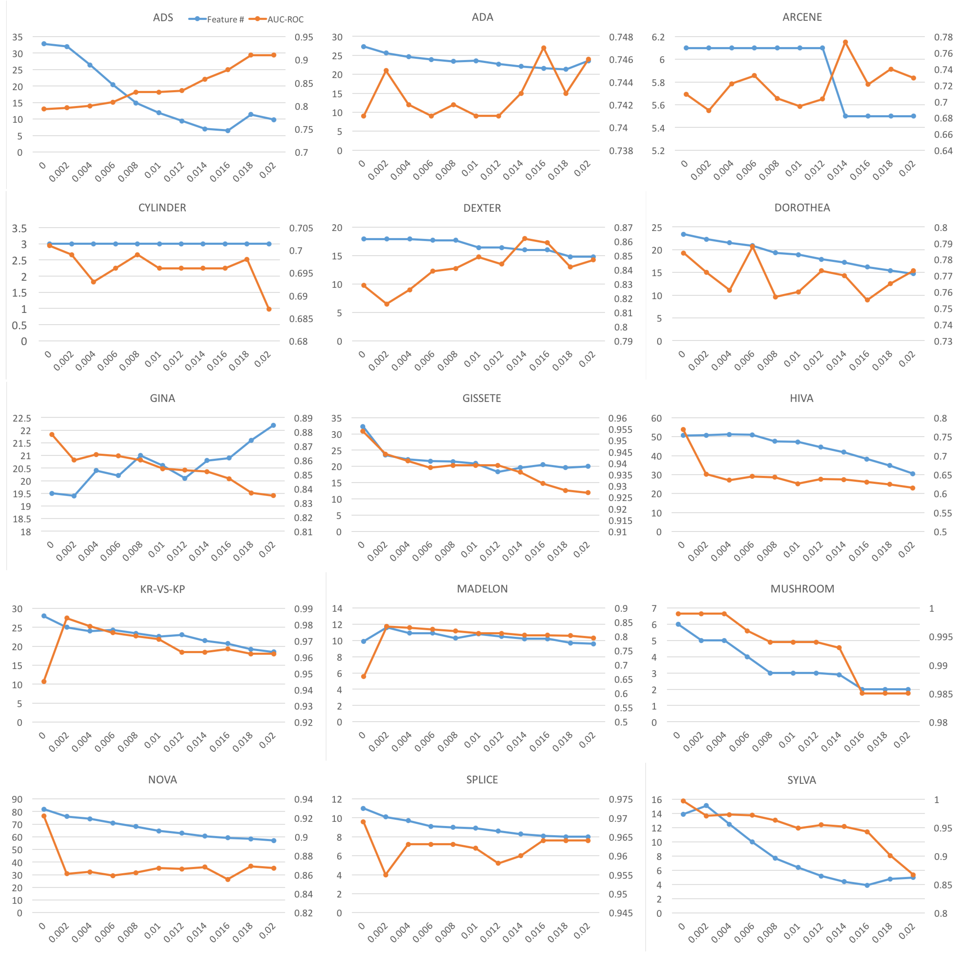
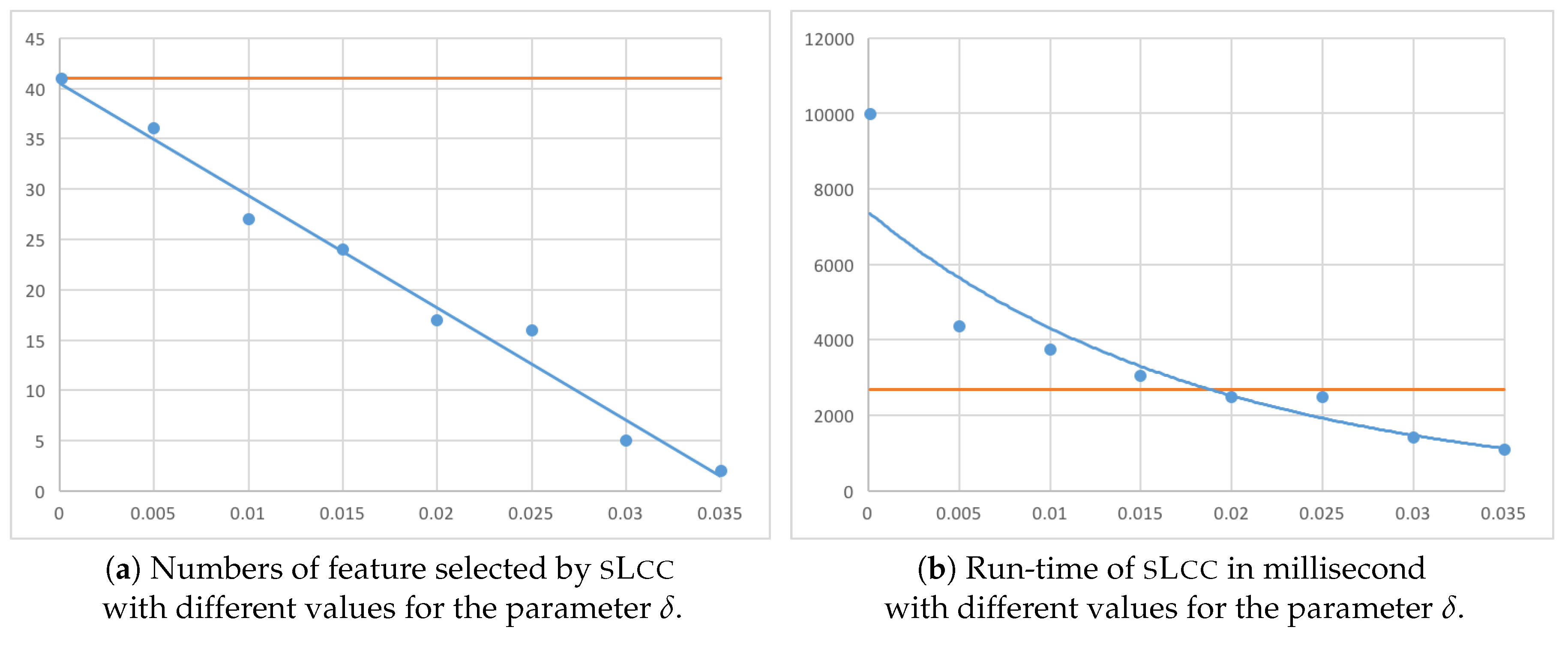
Lastly, we investigate how the parameter δ can affect the performance of sLcc. As described in Section 4.3, with greater δ , sLcc will eliminate more features, and, consequently, the run-time will decrease. To verify this, we run an experiment with sLcc with the dataset with 161,425 instances and 38,822 features. 
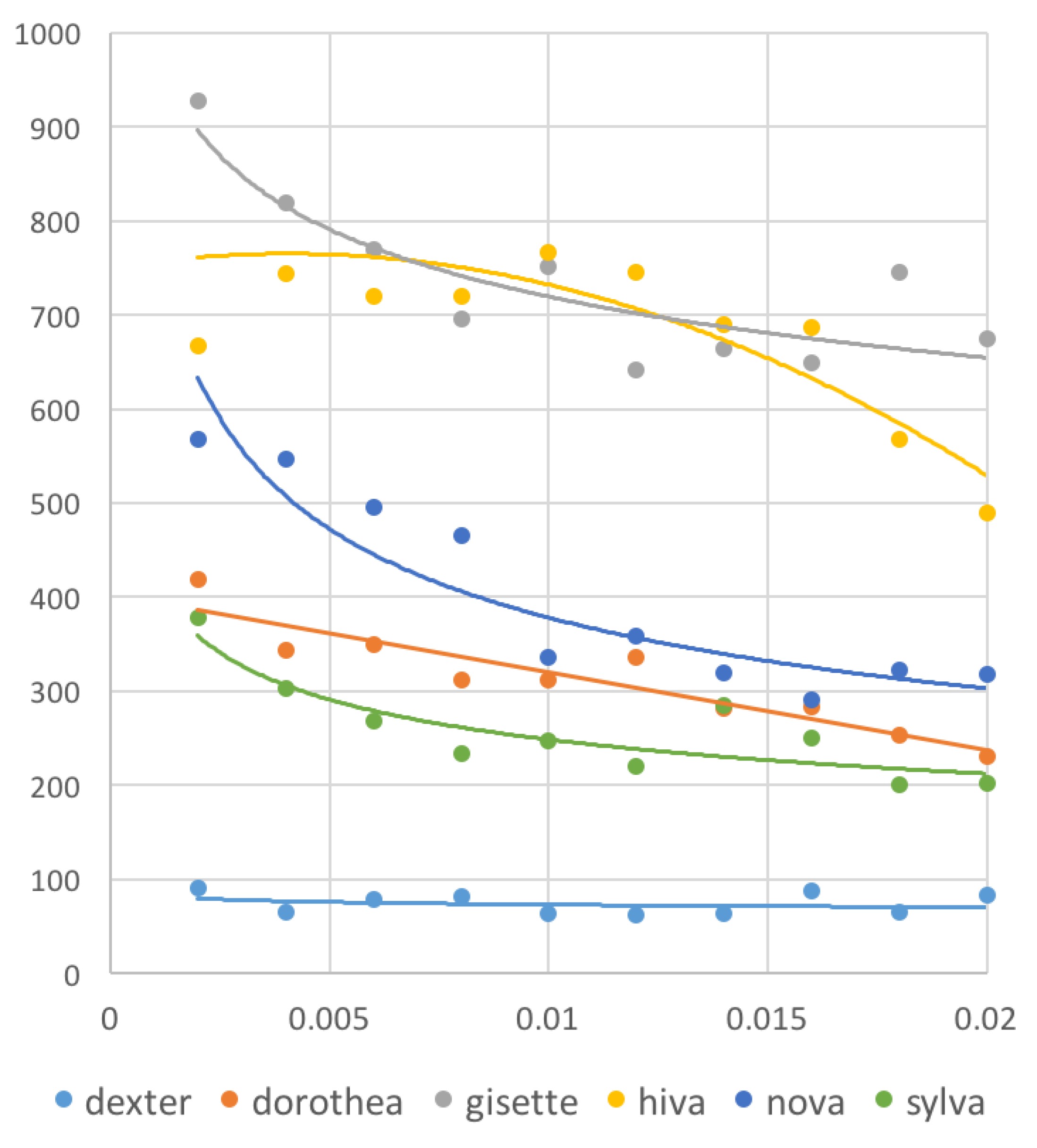
Figure 10 exhibits plots of the results. In fact, the number of features selected by and the run-time of sLcc decrease as the threshold δ increases. In addition, we see that, although sLcc selects the same features as sCwc when δ = 0 , the run-time is greater than sCwc. This is because computing the Bayesian risk (Br) is computationally heavier than computing the binary consistency measure (Bn). It is also interesting to note that sLcc becomes faster than sCwc for greater thresholds, and their averaged run-time performance appears comparable.

6. An Implementation

In this section, we show an implementation of our algorithms, which is also used in the experiments stated above. The data structure deployed by the implementation is a secret ingredient that makes the implementation fast. In addition, parallel computation will be possible thanks to the data structure.

6.1. The Data Structure

We consider the moment when sCwc selected F k 1 , F k 2 , , F k 1 in this order and has just decided to select the feature F k . We let F k = F k and call the sequence ( F k , F k 1 , , F k 1 ) a prefix. Note that k 1 < k 2 < < k = k holds. In the next round, F k + 1 , F k + 2 , , F N are targets of investigation. Hence, sCwc selects one of F k + 1 , F k + 2 , , F N , denoted by F k + 1 , and eliminates all of F k + 1 , F k + 2 , , F k + 1 1 .
In our implementation of sLcc and sCwc, at this moment, every instance of a dataset is represented as a vector of values for the sequence of features ( F k , F k 1 , , F k 1 , F N , F N 1 , , F k + 2 , F k + 1 ) , a concatenation of the prefix and the target features, and all of the instances are aligned in the lexicographical order of the feature values.
Figure 11 shows an example. In the example, the prefix is ( F 5 , F 3 , F 2 ) , and the targets in the next round are F 9 , F 8 , F 7 , F 6 . For simplicity, we assume that all of the features and the class are binary variables, which take either 0 or 1 as values. The Count column shows the number of instances that are identical in all of the remaining features ( F 2 , F 3 , F 5 , F 6 , F 7 , F 8 and F 9 ) and the class.
The following are advantages of this data structure. To illustrate, we let
S = { F k , F k 1 , , F k 1 , F N , F N 1 , , F k + 1 } .
  • To find inconsistent pairs of instances with respect to S, we only have to compare adjacent vectors (rows) in the data structure. We say that two instances compose an inconsistent pair with respect to S, if, and only if, the instances have the same value for every feature in S but are different in class labels.
  • To evaluate Br ( S { F k + 1 , , F i } ) and Bn ( S { F k + 1 , , F i } ) , we only have to evaluate the measures in the reduced data structure obtained by simply eliminating the columns that correspond to F k + 1 , , F i . In the reduced data structure, instances are still aligned in the lexicographical order of values with respect to ( F k , F k 1 , , F k 1 , F N , F N 1 , , F i + 2 , F i + 1 ) , and, hence, by investing adjacent vectors (rows), we can evaluate the measures.
  • Assume that the algorithm selects F k + 1 and eliminates the features F k + 1 , F k + 2 , , F k + 1 1 . The necessary update of the data structure can be carried out in time linear to the number of instances: first, we simply eliminate the columns corresponding to F k + 1 , F k + 2 , , F k + 1 1 ; in the reduced data structure, instances are aligned in the lexicographical order of values with respect to ( F k , F k 1 , , F k 1 , F N , F N 1 , , F k + 1 ) ; to update the prefix from ( F k , F k 1 , , F k 1 ) to ( F k + 1 , F k , , F k 1 ) , we only have to apply the bucket sort with respect to the value of F k + 1 .
For the example of Figure 11, Bn ( F 5 , F 3 , F 2 , F 9 , F 8 , F 7 , F 6 ) = 0 is derived, since no adjacent vectors are congruent with respect to the features F 5 , F 3 , F 2 , F 9 , F 8 , F 7 , F 6 .
Next, to evaluate Bn ( F 5 , F 3 , F 2 , F 9 , F 8 ) , we temporarily eliminate the columns of F 6 and F 7 . Figure 12 shows the resulting data structure. By investigating adjacent vectors (rows), we see that the first and second instances are inconsistent with each other with respect to the features F 5 , F 3 , F 2 , F 9 , F 8 . Hence, we have Bn ( F 5 , F 3 , F 2 , F 9 , F 8 ) = 1 .
Since we can verify Bn ( F 5 , F 3 , F 2 , F 9 , F 8 , F 7 ) = 0 by the same means, sCwc selects F 7 and eliminates F 6 . The left chart of Figure 13 shows the resulting data structure after eliminating F 6 ( F 7 is moved to the top of the prefix), while the right chart exhibits the result of applying bucket sort according to the value of F 7 . We should note that the vectors are aligned in the lexicographical order of the values of ( F 7 , F 5 , F 3 , F 2 , F 9 , F 8 ) , and the data structure is ready to go to the next round of selection.

6.2. The Program spcwc.jar

Instructions for using this program, namely spcwc.jar, are given in Table 15. The program contains implementation of both sCwc and sLcc. Using sLcc requires specifying a threshold value, which should be between Br ( F 1 , , F N ) and Br ( ) , where F 1 , , F N are the entire features of a dataset. Br ( ) is given by
Br ( ) = 1 max y Pr [ C = y ] .
sLcc returns the entire set { F 1 , , F N } when δ < Br ( F 1 , , F N ) , while it returns the empty set when δ Br ( ) .
In addition, we may change the measure used to sort features in the first step of sCwc and sLcc. Different feature selection results can be obtained with different measures. The measure can be either symmetrical uncertainty (default), mutual information, Bayesian risk, or Matthews correlation coefficient.
The program also outputs a log file with the extension .log. This log file contains the run-time record of the program, the features selected, the numbers of instances and features of the dataset input, and the measurements of individual features in the symmetrical uncertainty, the mutual information, the Bayesian risk and Matthews correlation coefficient.
The recommended method for using the program is to run it first with only the i option. Features will be sorted according to their symmetrical uncertainty scores, and, then, sCwc will select features. If we are not satisfied with the program’s result, we can try other options; for example, we can try sLcc with optimized threshold values. To obtain optimized threshold, we can take advantage of any methods for hyper-parameter optimization such as the grid search and the Bayesian optimization [18].

6.3. Parallelization

Another important advantage of the data structure described in Section 6.1 is its suitability for parallel computing. Since evaluation of the Bayesian risk and the binary consistency measure can be performed only by investigating whether adjacent instances are inconsistent with each other, we can partition the entire data structure into multiple partitions and can investigate them in parallel. The data structure must be partitioned so that two adjacent instances that belong to different partitions are not congruent with respect to values of the current features because such adjacent instances cannot be inconsistent.
For example, to evaluate Bn ( F 5 , F 3 , F 2 , F 9 , F 8 ) in Figure 12, we can partition the data structure of Figure 12 as Figure 14 depicts and investigate the partitions in parallel: Bn ( F 5 , F 3 , F 2 , F 9 , F 8 ) = 0 holds, if, and only if, any of the partitions includes no adjacent instances that are mutually inconsistent. For example, the first three instances of Figure 12 must belong to the same partition because they have identical values for the features F 5 , F 3 , F 2 , F 9 , F 8 .

7. Conclusions

Feature selection is a useful tool for data analysis, and, in particular, is useful to interpret phenomena that you find in data. Consequently, feature selection has been studied intensively in machine learning research, and multiple algorithms that exhibit excellent accuracy have been developed. Nevertheless, such algorithms are seldom used for analyzing huge data because the algorithms usually take too much time. In this paper, we have introduced two new feature selection algorithms, namely sCwc and sLcc, that scale well to huge data. They are based on the algorithms that exhibited excellent accuracy in the literature and do not harm the accuracy of the original algorithms. We have also introduced an implementation of our new algorithms and have described a recommended usage of the implementation.

Acknowledgments

This work was partially supported by the Grant-in-Aid for Scientific Research (KAKENHI Grant Number 16K12491, 17H00762 and 26280090) from the Japan Society for the Promotion of Science.

Author Contributions

This research started when Kuboyama discovered the fact that Cwc can run faster when it deploys a forward selection approach instead of a backward elimination approach. This discovery was supported by the observation that Cwc tends to eliminate many features before it selects the first feature. After an intensive discussion between Shin and Kuboyama, they reached the algorithm of sCwc, which deploys binary search, and as a result, has a significantly improved time complexity. Furthermore, Shin extended the result to Lcc and developed the algorithm of sLcc, which is as fast as sCwc and shows better accuracy performance. Shin and Kuboyama collaborated to implement the algorithms. Hashimoto generated the SNS datasets to use in their experiments and conducted the experiments collaboratively with Shin. Shepard applied the algorithms to real problems that involved large scale data and provided valuable comments, which contributed to the improvement of the algorithms. Shin wrote this paper.

Conflicts of Interest

The authors declare no conflict of interest.

References

  1. Almuallim, H.; Dietterich, T.G. Learning boolean concepts in the presence of many irrelevant features. Artif. Intell. 1994, 69, 279–305. [Google Scholar]
  2. Liu, H.; Motoda, H.; Dash, M. A monotonic measure for optimal feature selection. In Proceedings of the European Conference on Machine Learning, Chemnitz, Germany, 21–23 April 1998. [Google Scholar]
  3. Zhao, Z.; Liu, H. Searching for Interacting Features. In Proceedings of the International Joint Conference on Artificial Intelligence, Hyderabad, India, 6–12 January 2007; pp. 1156–1161. [Google Scholar]
  4. Shin, K.; Xu, X. Consistency-based feature selection. In Proceedings of the 13th International Conferece on Knowledge-Based and Intelligent Information & Engineering System, Santiago, Chile, 28–30 September 2009. [Google Scholar]
  5. Shin, K.; Fernandes, D.; Miyazaki, S. Consistency Measures for Feature Selection: A Formal Definition, Relative Sensitivity Comparison, and a Fast Algorithm. In Proceedings of the 22nd International Joint Conference on Artificial Intelligence, Barcelona, Spain, 16–22 July 2011; pp. 1491–1497. [Google Scholar]
  6. Kononenko, I. Estimating Attributes: Analysis and Extension of RELIEF; Springer: Berlin/Heidelberg, Germany, 1994. [Google Scholar]
  7. Peng, H.; Long, F.; Ding, C. Feature selection based on mutual information: Criteria of max-dependency, max-relevance and min-redundancy. IEEE Trans. Pattern Anal. Mach. Intell. 2005, 27, 1226–1238. [Google Scholar] [CrossRef] [PubMed]
  8. Yu, L.; Liu, H. Feature selection for high-dimensional data: A fast correlation-based filter solution. In Proceedings of the Twentieth International Conference on Machine Learning, Washington, DC, USA, 21–24 August 2003. [Google Scholar]
  9. Hall, M.A. Correlation-based feature selection for discrete and numeric class machine learning. In Proceedings of the Seventeenth International Conference on Machine Learning (ICML 2000), Stanford, CA, USA, 29 June–2 July 2000. [Google Scholar]
  10. Wang, G.; Song, Q.; Xu, B.; Zhou, Y. Selecting feature subset for high dimensional data via the propositional FOIL rules. Pattern Recognit. 2013, 46, 199–214. [Google Scholar] [CrossRef]
  11. Quinlan, J.; Cameron-Jones, R. FOIL: A midterm report. In Proceedings of the European Conference on Machine Learning, Vienna, Austria, 5–7 April 1993; Springer: Berlin/Heidelberg, Germany, 1993; pp. 1–20. [Google Scholar]
  12. Shin, K.; Miyazaki, S. A Fast and Accurate Feature Selection Algorithm based on Binary Consistency Measure. Comput. Intell. 2016, 32, 646–667. [Google Scholar] [CrossRef]
  13. Kira, K.; Rendell, L. A practical approach to feature selection. In Proceedings of the 9th International Workshop on Machine Learning, Aberdeen, UK, 1–3 July 1992; pp. 249–256. [Google Scholar]
  14. Neural Information Processing Systems (NIPS). Neural Information Processing Systems Conference 2003: Feature Selection Challenge; NIPS: Grenada, Spain, 2003. [Google Scholar]
  15. World Congress on Computational Intelligence (WCCI). In Proceedings of the IEEE World Congress on Computational Intelligence 2006: Performance Prediction Challenge, Vancouver, BC, Canada, 16–21 July 2006.
  16. Blake, C.S.; Merz, C.J. UCI Repository of Machine Learning Databases; Technical Report; University of California: Irvine, CA, USA, 1998. [Google Scholar]
  17. Demšar, J. Statistical comparisons of classifiers over multiple data sets. J. Mach. Learn. Theory 2006, 7, 1–30. [Google Scholar]
  18. Snoek, J.; Larochelle, H.; Adams, R.P. Practical Bayesian Optimization of Machine Learning Algorithms. arXiv, 2012; arXiv:1206.2944. [Google Scholar]
Figure 1. Clustering of twitter data. (a) tweets between 2:00 p.m. and 3:00 p.m. of 11 March. The quake hit Japan at 2:46 p.m., and 97,977 authors who posted 351,491 tweets in total are plotted; (b) tweets between 3:00 p.m. and 4:00 p.m. of 11 March. Furthermore, 161,853 authors who posted 978,155 tweets in total are plotted.
Information 08 00159 g001
Figure 2. An example result of feature selection by Cwc: Word (Score, Rank). Scores and ranks are measured by the symmetrical uncertainty. The Japanese words in this figure are translated as “emergency” (9), “networks” (11), “utilize” (13”, “favor” (15), “bath” (18), “great tsunami warning” (19), “place” (24), “phone” (26), “evacuation” (28), “absolute” (32), “all” (34), “possible” (37), “information” (39), “like” (40), “preparation” (41), “Miyagi” (42), “possibility” (45), “thing” (52), “Hanshin Great Quake” (55), “notification” (62), “over” (63), “disaster mail telephone” (65), “friend” (71), “as if” (72), “coast” (73), “safety” (74), “tsunami” (75), “Chu-Etsu Quake” (106), “television” (112), “Ibaraki” (115), “shock of earthquake” (119), “worry” (125), “Mr.”, “Mrs.” or “Ms.” (141), “earthquake intensity” (146) and “seem” (167). The numbers within parentheses indicate the ranks of the words.
Information 08 00159 g002
Figure 3. Progress of feature selection.
Information 08 00159 g003
Figure 4. A relationship between N F N I ( log N F + log N I ) (the x-axis) and run-time of sCwc (the y-axis).
Information 08 00159 g004
Figure 5. The fifteen datasets used in the experiment. The blue plots () represent the five datasets used in the feature selection challenge of NIPS 2003 [14], while the red plots () do those used in the challenge of WCCI 2006 [15]. The other five are retrieved from the USI repository [16].
Information 08 00159 g005
Figure 6. Comparison in accuracy.
Information 08 00159 g006aInformation 08 00159 g006b
Figure 7. Ranking.
Figure 7. Ranking.
Information 08 00159 g007
Figure 8. The Area Under an Receiver Operating Characteristic Curve (AUC-ROC) scores and numbers of features selected by sLcc changing δ from 0.0 to 0.02 at interval of 0.002. The lines and plots in blue represent feature numbers, while those in orange do AUC-ROC scores.
Information 08 00159 g008
Figure 9. Relation between the run-time of sLcc and the value of δ . The x-axis represents the value of δ , while the y-axis does the run-time of sLcc in milliseconds.
Information 08 00159 g009
Figure 10. The effects of different values upon the threshold parameter δ . The x-axis represents the value of δ , while the y-axis represents (a) the number of feature selected by and (b) the run-time of sLcc. The orange lines indicate the corresponding values by sCwc.
Information 08 00159 g010
Figure 11. An example of data structure.
Information 08 00159 g011
Figure 12. Evaluating Bn ( F 5 , F 3 , F 2 , F 9 , F 8 ) .
Information 08 00159 g012
Figure 13. Eliminating F 6 and sorting with respect to the value of F 7 .
Information 08 00159 g013
Figure 14. An example of data structure.
Information 08 00159 g014
Table 1. An example dataset.
F 1 F 2 F 3 F 4 F 5 C
101110
110000
000110
101000
111101
010101
010011
000011
0.1890.1890.0490.0000.000 I ( F i , C )
Table 2. An example dataset.
F 1 F 2 F 3 F 4 F 5 F 6 C
1011110
1100010
0001100
1010010
1111011
0101001
0100101
0000101
0.1890.1890.0490.0000.0000.189 I ( F i , C )
Table 3. Run-time of sCwc when applied to real high-dimensional data.
# of Instances# of FeaturesRun-Time (ms)# of Instances# of FeaturesRun-Time (ms)
15,56815,741252993,86297,261189,018
16,31917,2213682103,063103,063233,562
22,54021,6672064108,715106,808247,292
22,54021,6843547142,811102,083310,531
23,03619,7237378150,40237,61049,303
26,31917,2212576150,51737,60154,149
34,12529,36712,189155,24437,65947,497
37,05726,93812,062161,42538,82272,298
44,47130,82855,581179,76599,930367,125
44,81232,72121,191183,978100,622401,111
45,28434,1237500184,10899,588458,469
48,34835,0568873185,325100,466391,873
52,40039,57026,770187,92998,562403,179
64,19348,8107017195,73699,339461,130
71,81449,97441,089195,88799,419394,033
90,79794,707162,052200,56999,672405,803
Table 4. Attributes of the 15 datasets used in the experiment for comparison of accuracy.
#Dataset# of Features# of InstancesReference
1Ada484147[15]
2Ads15583279[16]
3Arcene10,000100[14]
4Cylinder40512[16]
5Dexter20,000300[14]
6Dorothea100,000800[14]
7Gina9703153[15]
8Gisette50006000[14]
9Hiva16173845[15]
10Kr-vs-Kp363196[16]
11Madelon5002000[14]
12Mushroom228124[16]
13Nova16,9691754[15]
14Splice603192[16]
15Sylva21613,086[15]
Table 5. Support Vector Machine (SVM) and the Area Under an Receiver Operating Characteristic Curve (AUC-ROC). Av. denotes averaged values.
Dataset12345789101112131415Av.
Raw Scores
Lcc0.7480.9100.7730.7010.8620.8790.9520.6520.9920.8351.000.8690.9640.9730.865
Frfs0.7630.8390.6040.6430.7930.9560.9800.6880.9410.6051.000.8940.9730.9890.833
Cfs0.7450.8950.6500.5590.8550.8630.9120.6000.9370.7490.9900.8630.9470.8880.818
Relief0.7430.8730.5000.6810.7060.6210.5480.6410.9290.5651.000.5400.9560.9520.733
Fcbf0.7450.8840.5820.6370.7410.8170.9290.5960.9370.6020.9900.8160.9480.9030.795
Ranking
Lcc2.01.01.01.01.02.02.02.01.01.02.02.02.02.01.57
Frfs1.05.03.03.03.01.01.01.02.03.02.01.01.01.02.00
Cfs3.52.02.05.02.03.04.04.03.52.04.53.05.05.03.46
Relief5.04.05.02.05.05.05.03.05.05.02.05.03.03.04.07
Fcbf3.53.04.04.04.04.03.05.03.54.04.54.04.04.03.89
Table 6. SVM and F-Score.
Dataset12345789101112131415Av.
Raw Scores
Lcc0.8260.9650.7560.7130.8600.8790.9520.9610.9920.83610.000.9020.9630.9920.900
Frfs0.8480.9420.5780.6510.7890.9560.9800.9700.9430.60510.000.9270.9730.9960.868
Cfs0.8330.9620.6240.5110.8510.8630.9120.9600.9390.7490.9900.9000.9460.9830.859
Relief0.8270.9500.3730.6890.7040.5450.4020.9610.9270.50410.000.6510.9550.9900.748
Fcbf0.8360.9590.5320.6430.7270.8170.9290.9610.9390.6020.9900.8710.9470.9850.838
Ranking
Lcc5.01.01.01.01.02.02.03.01.01.02.02.02.02.01.85
Frfs1.05.03.03.03.01.01.01.02.03.02.01.01.01.02.00
Cfs3.02.02.05.02.03.04.05.03.52.04.53.05.05.03.50
Relief4.04.05.02.05.05.05.03.05.05.02.05.03.03.04.00
Fcbf2.03.04.04.04.04.03.03.03.54.04.54.04.04.03.64
Table 7. Naïve Bayes and AUC-ROC.
Dataset12345789101112131415Av.
Raw Scores
Lcc0.8910.9330.7550.7760.9100.9010.9540.7690.9450.6600.9990.9220.9730.9970.885
Frfs0.8870.9540.6400.9190.9030.9060.9550.8030.9650.6340.9990.9300.9780.9980.891
Cfs0.8780.9420.6820.7320.9520.8970.9640.7320.9560.6540.9920.9280.9680.9890.876
Relief0.8700.8510.7680.7150.7620.9010.9380.6880.9750.5720.9980.5420.9790.9970.825
Fcbf0.8920.9370.6410.5860.8580.8920.9660.7170.9560.6180.9920.8930.9680.9890.850
Ranking
Lcc2.04.02.02.02.02.54.02.05.01.01.53.03.02.52.61
Frfs3.01.05.01.03.01.03.01.02.03.01.51.02.01.02.00
Cfs4.02.03.03.01.04.02.03.03.52.04.52.04.54.53.07
Relief5.05.01.04.05.02.55.05.01.05.03.05.01.02.53.57
Fcbf1.03.04.05.04.05.01.04.03.54.04.54.04.54.53.71
Table 8. Naïve Bayes and F-Score.
Dataset12345789101112131415Av.
Raw Scores
Lcc0.8320.9450.6810.5880.8350.8240.8880.9460.8990.6290.9900.8890.9190.9870.857
Frfs0.8310.8040.5970.8510.7760.8220.8850.9640.9170.6050.9770.8990.9240.9790.845
Cfs0.7890.9520.5850.6220.8490.8180.9010.9460.9270.6120.9860.8890.9120.9790.841
Relief0.7720.8970.7370.6600.6590.8230.8730.8940.9220.5010.9550.6380.9270.9820.803
Fcbf0.8370.9480.5540.5440.7240.8170.9080.9510.9270.5990.9860.8570.9120.9810.825
Ranking
Lcc2.03.02.04.02.01.03.03.55.01.01.02.53.01.02.43
Frfs3.05.03.01.03.03.04.01.04.03.04.01.02.04.52.96
Cfs4.01.04.03.01.04.02.03.51.52.02.52.54.54.52.86
Relief5.04.01.02.05.02.05.05.03.05.05.05.01.02.03.57
Fcbf1.02.05.05.04.05.01.02.01.54.02.54.04.53.03.18
Table 9. C4.5 and AUC-ROC.
Dataset12345789101112131415Av.
Raw Scores
Lcc0.8490.9150.6420.50.8320.8410.930.6850.9970.75810.000.8250.9660.9850.838
Frfs0.8960.8790.6170.50.7850.9010.9560.6410.9790.62310.000.8860.980.9970.831
Cfs0.8640.9230.5550.5570.7830.8460.9320.6330.9630.7520.9930.8230.9630.9440.824
Relief0.840.8950.630.6840.740.8280.9370.6640.9760.57410.000.5160.9650.9860.803
Fcbf0.8610.8910.6120.520.7120.8340.9190.5840.9630.6160.9930.7670.9630.9450.787
Ranking
Lcc4.02.01.04.51.03.04.01.01.01.02.02.02.03.02.25
Frfs1.05.03.04.52.01.01.03.02.03.02.01.01.01.02.18
Cfs2.01.05.02.03.02.03.04.04.52.04.53.04.55.03.25
Relief5.03.02.01.04.05.02.02.03.05.02.05.03.02.03.14
Fcbf3.04.04.03.05.04.05.05.04.54.04.54.04.54.04.18
Table 10. C4.5 and F-Score.
Dataset12345789101112131415Av.
Raw Scores
Lcc0.8310.9660.5840.4140.7740.8080.9080.9610.9900.71210.000.8940.9560.9900.842
Frfs0.8510.9550.5660.4140.7480.8600.9310.9650.9440.60410.000.9110.9710.9930.837
Cfs0.8370.9650.5390.4330.7350.8160.9150.9570.9400.7100.9900.8590.9500.9830.831
Relief0.8180.9490.5940.5870.6990.8210.9220.9540.9270.50110.000.6230.9560.9910.810
Fcbf0.8310.9540.5180.4210.6660.7950.8950.9530.9400.5990.9900.8320.9500.9860.809
Ranking
Lcc3.51.02.04.51.04.04.02.01.01.02.02.02.53.02.39
Frfs1.03.03.04.52.01.01.01.02.03.02.01.01.01.01.89
Cfs2.02.04.02.03.03.03.03.03.52.04.53.04.55.03.18
Relief5.05.01.01.04.02.02.04.05.05.02.05.02.52.03.25
Fcbf3.54.05.03.05.05.05.05.03.54.04.54.04.54.04.29
Table 11. Overall comparison of the feature selection algorithms. The scores of the Area Under an Receiver Operating Characteristic Curve (AUC-ROC) and F-Score are the averaged values across the three classifiers and the 14 datasets. On the other hand, the averaged ranks are computed across all of the combinations of classifiers, accuracy measures and datasets. The Friedman and Hommel tests are conducted based on the averaged ranks computed here.
Averagep-Value
AUC-ROCF-ScoreRankFriedmanHommel
sLcc0.8620.86320.18 Ctrl
Frfs0.8520.85020.18 90.81 × 10 1
Cfs0.8390.84330.22 0.000 40.37 × 10 5
Relief-F0.7870.78730.60 10.91 × 10 8
Fcbf0.8110.82430.82 90.24 × 10 11
Table 12. Comparison of run-time (seconds) with relatively large datasets.
DatasetsLccsCwcFrfsCfsRelief-FFcbfLccCwcInteract
Dexter0.0630.120.4035.51591.82.3318354.6193
Dorothea0.310.682.313,90654414,102
Gisette0.750.8611.03,97835125.22035.21219
Hiva0.760.422.169323.103.1114.91.1215.5
Nova0.320.333.4450215.5705155749
Sylva0.250.535.5611.911.61.952.920.4973.25
Results of the Hommel Test
Averaged Rank1.02.72.53.8
p-ValuesCtrl.0.0250.0440.000
Table 13. AUC-ROC of sCwc when applied to real high-dimensional data.
# of Instances# of FeaturesAUC-ROC# of Instances# of FeaturesAUC-ROC
71,81449,9740.99344,47130,8280.986
52,40039,5700.97644,81232,7210.985
34,12529,3670.99145,28434,1230.955
22,54021,6840.98648,34835,0560.995
16,31917,2210.938161,42538,8220.988
15,56815,7410.976155,24437,6590.937
23,03619,7230.963150,51737,6010.990
37,05726,9380.971150,40237,6100.988
Averages67,08531,5400.976
Table 14. Run-time of sLcc and Frfs (CentOS release 5.11, Intel Xeon X5690 6-Cores 3.47 GHz, 198 GB memory).
# of Instances# of FeaturessCwc (s)Frfs (s)Ratio
190,79794,707121.62849.423.4
283,86297,261143.53249.822.6
3108,715104,808215.45891.627.3
Table 15. Usage of SPCWC.JAR.
OptionValuesDescription
-i<path>Path to the input attribute-relation file format (arff) file.
-a<algorithm>The feature selection algorithm to use.
cwcRun sCwc (default).
lccRun sLcc.
-t<number>A threshold value for sLcc.
The value should be in the interval [0,1).
When the value 0 is specified, sCwc will run, even if -a lcc is specified.
-s<measure>A statistical measure to use when sorting features.
suThe symmetrical uncertainty will be used (default).
miThe mutual information will be used.
brThe Bayesian risk will be used.
mcMatthews correlation coefficient will be used.

