Lateral Cross Localization Algorithm Using Orientation Angle for Improved Target Estimation in Near-Field Environments

Abstract

Passive positioning systems with a small aperture array exhibit poor accuracy of target estimation under strong interference in near-field environments. To improve this accuracy, we propose a novel cross localization algorithm for direction-finding using the orientation angle. Improved geometric and numerical target-positioning models are constructed after analyzing the mechanism of the conventional positioning algorithm. The target prediction equation is then derived using the constructed models, and the equation for nonlinear estimation is linearized using the Taylor series. An unbiased estimation of the target is obtained by optimizing the control of the iteration process, thus achieving an accurate positioning of the target. The performance of the proposed algorithm was evaluated in terms of its effectiveness and positioning accuracy under varying signal-to-noise conditions and orientation angle-measurement errors. Simulation results show that the proposed algorithm is capable of positioning the target effectively, and offers better positioning accuracy than traditional algorithms under the conditions of large orientation angle measurement errors or high-level background noise.

1. Introduction

The technology of signal location is widely used in radar, sonar, and navigation systems, and can be classified as active or passive location, with different targets. Passive location technology has a broad scope of development and application prospects in the military due to its concealed nature [1]. The targets can be positioned by a single receiving node or a multi-node network [2]. In comparison with the single-node localization, the multi-node network has a higher signal gain and target resolution. According to different implementation techniques, the positioning methods mainly include combining the space and time cumulative positioning [3], fusion azimuth, and time difference of arrival (TDOA) [4] positioning methods based on Doppler shift [5], multipath target motion analysis (TMA), signal strength, and line spectral characteristics [6,7]. Different monitoring environments and objectives require different positioning methods. For example, the methods that combine azimuth and TDOA are applied in situations where the sensor array aperture is comparable to the target distance, while the time-cumulative methods require a high-precision time reference. The methods based on azimuth and Doppler shift have high accuracy on high-frequency fast-moving targets [8,9,10].

This paper mainly focuses on near-field targeting technology in a small aperture array. By analyzing the characteristics of a near-field signal and a small aperture array, we propose a lateral cross localization algorithm using the signal orientation angle. The algorithm uses multiple orientation angles measured by different nodes to locate the target. To deal with the problem of nonlinear estimation, predictive equations are defined and linearized by Taylor series expansion. The parameters are estimated through Gauss-Newton iteration using maximum likelihood estimation, and the targets’ position is then obtained through optimal estimation. The proposed algorithm can improve the positioning accuracy of the orientation angle cross localization method effectively, especially under significant orientation error and complex background noise.

2. Problem Formulation

The optimal passive targeting method involves centralized global information processing. Each array sends the observed data to the fusion center, which estimates the target using the global information. Typical location algorithms based on complete information include the least squares algorithm [11], maximum likelihood algorithm [12], and the algorithm based on space-time subspace optimization [13]. Weiss [11] has reported the use of the L-base sensor array to receive radio frequency signals transmitted by a single transmitter, and using the least squares method to position the transmitter directly. Through maximizing the eigenvalues of an L × L matrix, the transmitter location can be obtained with a simple 2-D search algorithm. Another extended single-objective targeting for multiple transmitter positioning has been reported by Weiss et al. [11]. Another approach [13] uses the method of maximum likelihood and subspace optimization. The objective functions for the direct position of multiple transmitters include attenuation coefficient, signal source, target position, and other unknown parameters. The maximum likelihood method requires a multi-dimensional search, but the subspace optimization method is able to locate all targets with only a two-dimensional search. Methods reported in [11] and [13] have also considered situations where the signal waveform is known so that the optimization cost can be simplified to varying degrees.

Although the centralized global information processing method is theoretically optimal, its implementation process needs large communication bandwidth, computation, and energy consumption [14]. In practical applications, the positioning system for different scenarios is restricted by energy resources. For example, the positioning nodes deployed in harsh environments are powered by ordinary batteries and are often left unattended; thus, the energy of each node is extremely limited. Additionally, to achieve global information by directly targeting the algorithm, each array requires strict time synchronization [15]. For example, the approach in [13] assumes that the time synchronization level of each base station before positioning is 50 ns. Such high synchronization accuracy necessitates high demands of hardware and synchronization algorithms.

Under the premise of limited communication bandwidth and energy, researchers have proposed many resource-constrained wireless passive-targeting algorithms. Among these, the most common algorithm is based on azimuth [16,17]. These algorithms based on azimuth and their corresponding systems have been widely used due to their low resource consumption, and lower hardware and software requirement. Some examples include the Acoustic ENSBox at the California Institute of Technology [18,19,20], VoxNet [21], and an array system based on sound propagation delay compensation developed by Kaplan et al. [22,23].

Pure azimuth targeting is a simple and practical closed linear algorithm. The representative linear algorithms mainly include the Stansfield estimator [24] and the orthogonal vector (OV) algorithm [25]. If the weight matrix of the Stansfield estimator is replaced by a unit matrix, the Stansfield estimator becomes equivalent to the OV algorithm. The linear estimator offer advantages of being simple to compute and easy to implement. However, they suffer from limitations of low accuracy and estimator bias. With the increase in observed data, estimation deviation continues to exist and does not reduce. Therefore, several modifications to address this problem have been reported in the literature, such as instrumental variable (IV) [26,27,28], constrained least squares (CLS) [29], and total least squares (TLS) [30,31]. The IV estimator is consistent, progressive, and unbiased. Its root mean-square error (RMSE) is progressive and tends towards the Cramer–Rao lower bound (CRLB). Le Cadre and Jauffret proved that the convergence of the IV algorithm is very sensitive to the initial value and the selection of step [32]. Ho et al. proposed the CLS algorithm and conducted target motion analysis. The CLS algorithm has been proved to be progressive and unbiased. Gu [33] proved that the CLS algorithm is actually a progressive maximum-likelihood estimator. Similarly, the TLS algorithm is also a progressive maximum-likelihood estimator. CLS is simpler than TLS but it can only be used for a class of pseudo-linear models. By contrast, TLS can be applied to more universal models, such as angle observers. It should be noted that at low SNR, the position estimates of both CLS and TLS have a large RMSE. Additionally, with less measurement data, CLS serves as the approximation of the OV estimator.

The deviation of closed loop linear estimator can be eliminated by traditional bearing maximum-likelihood (TBML) estimator or nonlinear least squares. Gavish et al. [34] pointed out that the RMSE of a closed loop linear estimator may be smaller than the TBML estimator for limited observation data. When the amount of observation data is large enough, the TBML estimator has better performance than the closed-loop linear estimator. Assume that the angle observation noise obeys a Gaussian distribution with zero mean; the cost function of the TBML is nonlinear and non-convex. Therefore, the TBML problem is always solved by a gradient search, such as the Newton–Raphson iterative method.

In particular, the IV and numerical TBML iterative algorithms may be divergent under conditions such as poor initial value, fewer observations, or worse geometric positional relationship between the target and angle observer. Bishop et al. [35] proposed a new algorithm based on geometry constrained least squares (GCLS), which minimizes the angle observation error under the constraint of geometric positional relationship between the target and angle observer. This method is equivalent to TBML under Gaussian observation noise because the geometric constraints do not provide any additional information to the position estimate. However, the geometric constraints can aid the convergence of the nonlinear least-square algorithm on the basis of angle observation. In comparison with TBML, the GCLS could converge under poor geometric positional relationship between the target and the angle observer; moreover, CLS and TLS are simpler, and more effective with the increase in measurement data and in achieving maximum-likelihood estimation progressively. In the case of large observation error, the estimation accuracy of numerical TBML is higher than CLS and TLS, but the TBML diverges easily or converges only to a local minima in the cases mentioned above.

3. Lateral Cross Positioning System Model

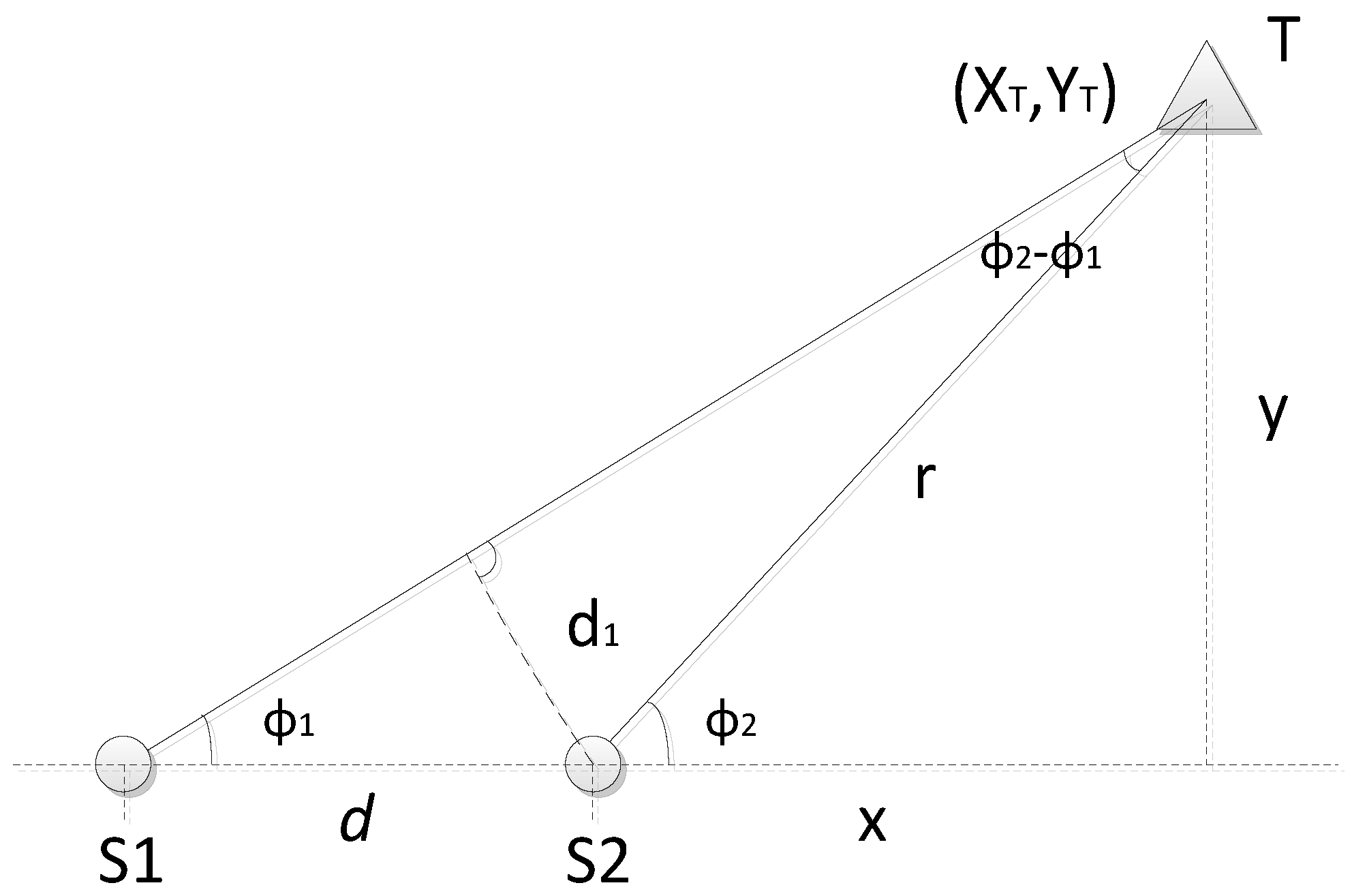
3.1. Description of Lateral Cross Positioning Method

The lateral cross positioning methods estimate targets with the signal orientation angle obtained by nodes. The positioning accuracy is determined by the direction-finding (DF) accuracy of the sensors. Assume that if multiple nodes detect the same target almost at the same time, we can obtain pluralities of the bearing lines [36]. Without loss of generality, we investigate the two-dimensional case first, and then extend the method to three-dimensional space. The measuring principle is shown in Figure 1.

Here S1, S2 are probe nodes, T is the target, and the distance between probe nodes is d. Then:

$$\sin {\varphi }_1=\frac{d_1}{d},\sin ({\varphi }_2-{\varphi }_1)=\frac{d_1}{r}$$

(1)

Thus:

$$r=\frac{d\sin {\varphi }_1}{\sin ({\varphi }_2-{\varphi }_1)}$$

(2)

Following (1) and (2), and the relationship shown in Figure 1, we obtain:

$$\{\begin{array}{l}x=\frac{d\sin {\varphi }_1\cos {\varphi }_2}{\sin ({\varphi }_2-{\varphi }_1)}\\ y=\frac{d\sin {\varphi }_1\sin {\varphi }_2}{\sin ({\varphi }_2-{\varphi }_1)}\end{array}$$

(3)

The position coordinates of the target can be calculated using Equation (3), and the method is suitable for multiple targets. In practical applications, there are measurement errors and noise in the target orientation angle that may produce a large deviation between the obtained and the actual position. By increasing the number of nodes, we can obtain more orientation lines and improve the positioning accuracy. With the presence of noise and error, these orientation lines do not always intersect at one point but stagger into an irregular polygon.

We first study three sensor nodes in a two-dimensional plane, where the three orientation lines intersect into a triangle. The position of the target is assumed to be the centroid of the triangle. The number of orientation lines is more than three in a three-dimensional space with a multiple-node array. In order to obtain more accurate results, we can first select three orientation lines to obtain a centroid, and then take the centroid (or mean) of different centroids. This paper mainly focuses on the single-target location problem in a three-dimensional space.

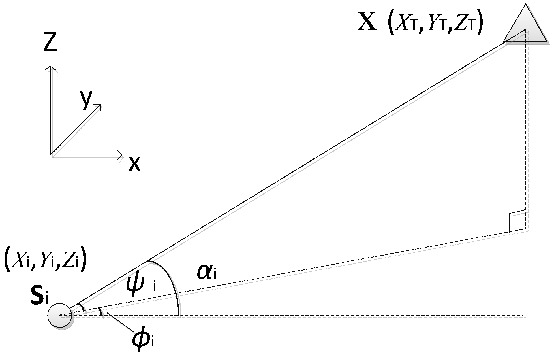
3.2. Targeting Model

Assume the coordinates of target to be estimated is x_T = [x_T, y_T, z_T]^T, the angles measured once by N nodes are {u_i, i = 1, 2, ..., N}, where u_i ∈ {φ_i, ϕ_i}, φ_i is the pitch angle, and ϕ_i is the azimuth angle. The schematic diagram is shown in Figure 2. For multiple nodes, set the coordinate vector as s_i = [x_i, y_i, z_i], the angle u_i can be obtained by the node coordinate values.

Since the measurement system contains additive random error, the system numerical model is always referred to as:

$$u_i=f_i(x_T)+n_i,(i=1,2,\cdots ,N)$$

(4)

where N is the number of detection nodes. Expressed in matrix form:

$$u=f(x_T)+n$$

(5)

If the measurement results do not contain errors, then $u_i=f_i(x_T)={\alpha }_i$ and the relationship between the orientation angle and target coordinates in $f_i(x_T)$ is nonlinear. Assuming that measurement error, n_i, follows the relation:

$$E\left\{n_i\right\}=0,E\left\{n_i{n}_j\right\}={\sigma }_{ij}$$

(6)

$${\sigma }_{ij}=\{\begin{array}{l}{\sigma }_i^2,i=j\\ {\rho }_{ij}{\sigma }_i{\sigma }_j,i\ne j\end{array}$$

(7)

where σ_i and σ_j are standard deviations in i^th and j^th monitoring experiments, ρ_ij is the correlation coefficient between position values. To solve the above nonlinear problem, first we need to linearize the prediction equations. We expand the equations according to Taylor series at reference point x_T0, where $x_{T0}={\left[x_{T0},y_{T0},z_{T0}\right]}^T$ is the initial estimate. We take the second (or first few-order terms) of the expanded series and obtain the fixed initial equation:

$$w_{oi}=u_i+g_{oi}^T{x}_T,(i=1,2,\cdots ,N)$$

(8)

where w_oi is the fixed measurement. The calculation formula, as follows:

$$w_{oi}=u_i+g_{oi}^T{x}_{T0}-f_{oi},(i=1,2,\cdots ,N)$$

(9)

where g_oi^T is the gradient of f_i(x_T) at point x_T0. It is defined as:

$$g_{oi}^T={\frac{\partial f_i(x_T)}{\partial x_T}|}_{x_T=x_{T0}}={\left[\frac{\partial f_i(x_T)}{\partial x_T}\frac{\partial f_i(x_T)}{\partial y_T}\frac{\partial f_i(x_T)}{\partial z_T}\right]}_{x_T=x_{T0}}$$

(10)

where f_oi is the value of f_oi (x_T) at x_T0 and f_oi = f_i (x_T0).

The N monitoring nodes have N initial relationships as obtained fromEquation (8); combining them into a matrix:

$$w_o=G_0{x}_T+n$$

(11)

where w_o is obtained by the following formula:

$$w_o=u+G_0{x}_T-f_0$$

(12)

Here, w_o, u, n, f₀ are N × 1 dimensional column vectors:

$$w_o={\left[w_{01},w_{02},\cdots ,w_{0i},\cdots ,w_{oN}\right]}^T$$

(13)

$$u_o={\left[u_{01},u_{02},\cdots ,u_{0i},\cdots ,u_{oN}\right]}^T$$

(14)

$$n_o={\left[n_{01},n_{02},\cdots ,n_{0i},\cdots ,n_{oN}\right]}^T$$

(15)

$$f_o={\left[f_{01},f_{02},\cdots ,f_{0i},\cdots ,f_{oN}\right]}^T$$

(16)

G₀ is an N × 3 dimensional gradient matrix, whose i^th row is a 1 × 3 dimensional gradient vector ${\mathrm{g}}_{\text{oi}}^{\mathrm{T}}$, or i^th column of ${\mathrm{G}}_0^{\mathrm{T}}$ is a 1 × 3 dimensional gradient vector ${\mathrm{g}}_{\text{oi}}$ Therefore:

$$G_o={\left[g_{01},g_{02},\cdots ,g_{oi},\cdots ,g_{oN}\right]}^T$$

(17)

where the error vector n meets the criterion:

$$E\left\{n\right\}=0,E\left\{n{n}^T\right\}=R$$

(18)

in which R ∈ V (N × N) is measurement error covariance matrix, n is Gaussian random variable. The maximum likelihood estimation ${\widehat{x}}_{\mathrm{T}}$ of the target position vector $x_{\mathrm{T}}$ can be solved by Gauss-Newton iterative. The procedure is:

$${\widehat{x}}_{T,m+1}={(G_m^T{R}^{-1}{G}_m)}^{-1}{G}_m^T{R}^{-1}{w}_m,m=0,1,2,\cdots$$

(19)

where m is the iterations count. $w_m,G_m$ are:

$$w_m=u+G_m{\widehat{x}}_{T,m}-f_m$$

(20)

$$w_m=u+G_m={\frac{\partial f(x_T)}{\partial x_T}|}_{x_T={\widehat{x}}_{T,m}},f_m=f({\widehat{x}}_{T,m})$$

(21)

Take ${\widehat{x}}_{T,m}$ obtained at each iteration as the initial value $x_{T0}$ for the next iteration. Note that $x_T$ obtained in initial iteration is ${\widehat{x}}_{T,1}$. According to Equation (19):

$${\widehat{x}}_{T,1}={(G_0^T{R}^{-1}{G}_0)}^{-1}{G}_0^T{R}^{-1}{w}_0$$

(22)

where m = 0. Thus, the target values are a series of revised estimation sequence:

$$x_{T0},{\widehat{x}}_{T,1},{\widehat{x}}_{T,2},\cdots ,{\widehat{x}}_{T,m},{\widehat{x}}_{T,m+1}\cdots$$

(23)

If the initial point $x_{T0}$ of the iterative process is near the global minimum point of the squared weighted cost function as following:

$$S(x_T)=n^T{R}^{-1}n={\left[u-f(x_T)\right]}^T{R}^{-1}\left[u-f(x_T)\right]$$

(24)

and satisfies the iteration convergence conditions, then the final estimates are given as:

$${\widehat{x}}_T=\underset{m\to \infty }{\lim }{\widehat{x}}_{T,m}$$

(25)

In practical applications, the commencement and termination of the iterative process are controlled by a threshold, and we study these guidelines in the following algorithm.

4. Proposed Lateral Cross Localization Algorithm Using Orientation Angle

4.1. Description of the Proposed Algorithm

For the targeting-related issues in a three-dimensional space, we study the orientation angle α on the basis of azimuth and pitch angle, as shown in Figure 2. The relationship between α and ϕ, φ is:

$$\alpha =\arctan \sqrt{{\tan }^2\phi +{\tan }^2\varphi }$$

(26)

or

$$\alpha =\arccos \sqrt{\cos \phi \cos \varphi }$$

(27)

Then for the i^th node $s_i=[x_i,y_i,z_i]$, i = 1, 2, …, N, the relationship with target $x_T={[x_T,y_T,z_T]}^T$ is:

$$f_i(x_T)={\alpha }_i=\arctan \frac{\sqrt{{(x_T-x_i)}^2+{(z_T-z_i)}^2}}{y_T-y_i}$$

(28)

When the number of iteration is m, the gradient vector is:

$$g_{mi}={\left[\frac{{\widehat{x}}_m-x_i}{r_{mi}^2{s}_{mi}}-\frac{{\widehat{y}}_m-y_i}{r_{mi}^2{s}_{mi}}\frac{{\widehat{z}}_m-z_i}{r_{mi}^2{s}_{mi}}\right]}^T$$

(29)

where

$$r_{mi}^2={({\widehat{x}}_m-x_i)}^2+{({\widehat{y}}_m-y_i)}^2+{({\widehat{z}}_m-z_i)}^2$$

(30)

$$s_{mi}=\sqrt{{(\frac{r_{mi}}{{\widehat{y}}_m-y_i})}^2-1}$$

(31)

The N gradient vectors constitute a gradient matrix:

$$G_m={\left[g_{m1},g_{m2},\cdots ,g_{mN}\right]}^T$$

(32)

The covariance matrix of orientation angle error in the m^th iteration is an N × N dimensional diagonal matrix. Diagonal elements of the matrix vary with the iterative equation, which is:

$$R_m=\mathrm{diag}{\left[{\sigma }_{m1}^2,{\sigma }_{m2}^2,\cdots ,{\sigma }_{mN}^2\right]}^T$$

(33)

where ${\sigma }_{mi}^2$ is error variance of orientation angle in m^th iteration. The solution is:

$${\sigma }_{mi}^2=a_{mi}{\sigma }_{\varphi i}^2+b_{mi}{\sigma }_{\phi i}^2+c_{mi}{\rho }_i{\sigma }_{\varphi i}{\sigma }_{\phi i}$$

(34)

where

$$a_{mi}={(\frac{1}{s_{mi}}\frac{{\widehat{x}}_m-x_i}{{\widehat{y}}_m-y_i})}^2$$

(35)

$$b_{mi}={\left\{s_{mi}{\left[(\frac{r_{mi}}{{\widehat{z}}_m-z_i})-1\right]}^{1/2}\right\}}^{-2}$$

(36)

$$c_{mi}=\sqrt{a_{mi}{b}_{mi}}$$

(37)

Assuming that the ambient noise is additive Gaussian white noise, the iterative equation can be expressed as:

$${\widehat{x}}_{T,m+1}={(G_m^T{R}_m^{-1}{G}_m)}^{-1}{G}_m^T{R}_m^{-1}{w}_m$$

(38)

where

$$w_m=u+G_m{\widehat{x}}_{T,m}-f({\widehat{x}}_{T,m})$$

(39)

in which $f({\widehat{x}}_{T,m})$ is the value of $f(x_T)$ at $x_T=x_{T,m}$.

4.2. Iterative Process Control

For the iterative process, we need to first analyze the value of initialization estimate $x_{T0}$ of position vector $x_T$. The value methods of $x_{T0}$ mainly include experience speculation and rough calculation on measurements. Here, the initialization estimate is received through solving the intersection of a group of orientation angle in observation surface.

Assume that the orientation angles of a set of known measurements $\{{\phi }_i,{\phi }_j,{\varphi }_k\}$ intersect at point $x_{ijk}$, such that i ≠ j and k = i, j or k ≠ i, j. The intersection point can be determined by the equation set below:

$$\{\begin{array}{l}{\phi }_i=\arctan \frac{x-x_i}{y-y_i}\\ {\phi }_j=\arctan \frac{x-x_j}{y-y_j}\\ {\varphi }_j=\arctan \frac{z-z_j}{\sqrt{{(x-x_j)}^2+{(y-y_j)}^2}}\end{array}$$

(40)

The solution of the equation can be expressed as:

$$x_{ijk}={\left[x_{ij} y_{ij} z_{ijk}\right]}^T$$

(41)

where

$$\{\begin{array}{l}{x}_{ij}=\frac{(y_i-y_j)a_{ij}+x_j{a}_{ij}+x_i{d}_{ij}}{\sin ({\phi }_i-{\phi }_j)}\\ y_{ij}=\frac{(x_i-x_j)b_{ij}+y_j{c}_{ij}+y_i{d}_{ij}}{\sin ({\phi }_i-{\phi }_j)}\\ z_{ijk}=z_k+\sqrt{{(x_{ij}-x_k)}^2+{(y_{ij}-y_k)}^2}\tan {\varphi }_k\end{array}$$

(42)

By analysis of the target space, we obtain:

$$\{\begin{array}{l}{a}_{ij}=\sin {\phi }_i\sin {\phi }_j\\ b_{ij}=\cos {\phi }_i\cos {\phi }_j\\ c_{ij}=\sin {\phi }_i\cos {\phi }_j\\ d_{ij}=\cos {\phi }_i\sin {\phi }_j\end{array}$$

(43)

Here, $x_{ijk}$ is initialization priori information, that is:

$$x_{T0}=x_{ijk}$$

(44)

For iterative process control, the threshold should satisfy some criterion of positioning accuracy:

$$D(\Delta {\widehat{x}}_{T,m})=\{\begin{array}{l}A, {(\Delta {\widehat{x}}_{T,m})}^T\Delta {\widehat{x}}_{T,m}\le {\zeta }^2\\ B, {(\Delta {\widehat{x}}_{T,m})}^T\Delta {\widehat{x}}_{T,m}>{\zeta }^2\end{array}$$

(45)

where D is the control instruction, A and B are the termination and continuation of the iterative process, respectively, ζ is the estimation accuracy, and $\Delta {\widehat{x}}_{T,m}$ is the difference between two estimated values:

$$\Delta {\widehat{x}}_{T,m}={\widehat{x}}_{T,m+1}-{\widehat{x}}_{T,m}$$

(46)

4.3. Analysis of Estimation Error

An error in location refers to the deviation between the estimated value ${\widehat{x}}_T$ and actual value $x_T$ of the target position. After the (m + 1)^th iteration, the error vector covariance matrix of the position vector $x_T$ is:

$$R_{{\widehat{x}}_{T,m+1}}={(G_m^T{R}_m^{-1}{G}_m)}^{-1}$$

(47)

where R_m is the covariance matrix of the pre-observation estimation error for describing the error in the position estimation.

This algorithm locates the target based on orientation angles obtained by sensor nodes. The influence on positioning is due to various factors such as measurement error and noise, and concentrated expression in orientation angle error. For the positioning system shown in Figure 2, assume Gaussian white noise n_k exists with zero mean and variance ${\sigma }_n^2$, deviation ϕ with zero mean, and variance ${\sigma }_{\varphi }^2$. We obtain:

$$E\left\{n_i{n}_k\right\}={\sigma }_n^2{\delta }_{jk}$$

(48)

The observations of orientation angles are:

$${\varphi }_k=\arctan (\frac{\Delta y_k}{\Delta x_k})+\varphi +n_k,k=1,2,\cdots ,N$$

(49)

where $\Delta y_k=y_T-y_k$, $\Delta x_k=x_T-x_k$. Define $\mathsf{\theta }={[x_T,y_T,\varphi ]}^T$ as the estimate vector. Here, θ obeys the multidimensional normal distribution with mean vector, m, and positive definite covariance matrix Σ. Define h(m, θ) = 0 as constraint vector, and:

$$h_m=\frac{\partial h}{\partial m},h_{\theta }=\frac{\partial h}{\partial \mathsf{\theta }}$$

(50)

For vector θ with predict prior information, its CRLB is:

$$S_{\theta }={\left[h_{\theta }^T{(h_m{\displaystyle \sum h_m^T})}^{-1}{h}_{\theta }+J\right]}^{-1}$$

(51)

Assume variance ${\mathbf{\sigma }}_{\varphi }^2$ of deviation is known and is non-zero, then:

$$J=\left[\begin{array}{ccc}0& 0& 0\\ 0& 0& 0\\ 0& 0& 1/{\sigma }_{\varphi }^2\end{array}\right]$$

(52)

Differentiate formula (49) on the estimator θ, then:

$$h_{\theta }=\left[\begin{array}{cc}G& I_N\end{array}\right]$$

(53)

where

$$G={\left[\begin{array}{cccc}-\frac{\Delta y_1}{r_1^2}& -\frac{\Delta y_2}{r_2^2}& \cdots & -\frac{\Delta y_N}{r_N^2}\\ -\frac{\Delta x_1}{r_1^2}& -\frac{\Delta x_2}{r_2^2}& \cdots & -\frac{\Delta x_N}{r_N^2}\end{array}\right]}^T$$

(54)

$$r_k^2={\Delta }_{xk}^2+{\Delta }_{yk}^2,k=1,2,\cdots ,N$$

(55)

$I_N$ is a vector consisting of N – 1 elements; h_m and σ⁻² Σ are N × N dimensional unit matrix as the noise covariance matrix satisfies the diagonal structure.

$$\begin{array}{cc}\hfill S_{\theta }=& {\left[{\left[G I_N\right]}^T{({\sigma }_n^2{I}_N)}^{-1}\left[G I_N\right]+diag(0,0,{\sigma }_{\varphi }^{-2})\right]}^{-1}\hfill \\ \hfill =& {\sigma }_{\varphi }^2{\left[\begin{array}{cc}{V}^{-1}& f\\ f^T& {({\sigma }_n/{\sigma }_{\varphi })}^2+N\end{array}\right]}^{-1}\hfill \end{array}$$

(56)

where $f=G^T{I}_N,V={(G^{T}G)}^{-1}$. The upper left corner 2 × 2 subarray of S_θ is the target estimation CRLB. Inversing the partitioned matrix:

$$S_{\theta }={\sigma }_n^2(V+\frac{Vf{f}^{T}V}{{({\sigma }_n/{\sigma }_{\varphi })}^2+N-f^{T}Vf})$$

(57)

Since the priori bias may be infinite, we get:

$$S_{\max }=\underset{{\sigma }_{\varphi }\to \infty }{\lim }{S}_{\theta }={\sigma }_n^2(V+\frac{Vf{f}^{T}V}{N-f^{T}Vf})$$

(58)

Here, S_θ ≤ S_max shows the influence of deviation with prior information. The error range is defined as:

$$S_{\theta }={\sigma }_n^2,\hspace{1em}{\sigma }_{\varphi }\to 0$$

(59)

5. Performance Analysis

We analyze the performance of the proposed algorithm through simulations. Positioning methods using a lateral cross mainly includes direct measurement, least squares, and their extensions. We compare the performance of the direct lateral cross localization algorithm (Algorithm 1), linear least-squares localization algorithm (Algorithm 2), and the proposed lateral cross localization algorithm based on orientation angle (Algorithm 3).

The number of Monte Carlo simulation run time is N = 5000. The localization precision is expressed in terms of RMSE as:

$$RMSE(u)={\displaystyle \sum _{i=1}^N\Vert (u^{(i)}-u)\Vert /N m}$$

(60)

where u⁽ⁱ⁾ is the i^th target estimation, and the environmental noise is assumed to have a Gaussian distribution. We investigate how the localization precision changes with orientation angle measurement error and SNR. The nodes position (in m) are set as s₁(0, 0, 0), s₂(20, 0, 0), s₃(26, 15, 0), s₄(37, −10, 8), and s₅(60, 20, −20), and the target position is set as T(800, 800, 400).

5.1. Algorithm Effectiveness

We locate the target once with different algorithms to test the effectiveness of the single-positioning experiment. Here SNR = 10 dB and the positional deviation results are shown in

Table 1. Comparison of targeting results from different algorithms.

Algorithm	Absolute Deviation of Estimated Position (m)
	x	y	z
Algorithm 1	1.9	2.1	0.8
Algorithm 2	1.4	1.5	0.7
Algorithm 3	0.6	0.8	0.2

.

As displayed the Table 1, under the same simulation environment, all three algorithms are able to locate the target. The positional deviations of different algorithms on the three axes have a significant proportional relationship with the distance of the observation node from the target in that axis. Comparing with Algorithm 1 and Algorithm 2, Algorithm 3 has a smaller deviation, which shows Algorithm 3 has better positioning accuracy.

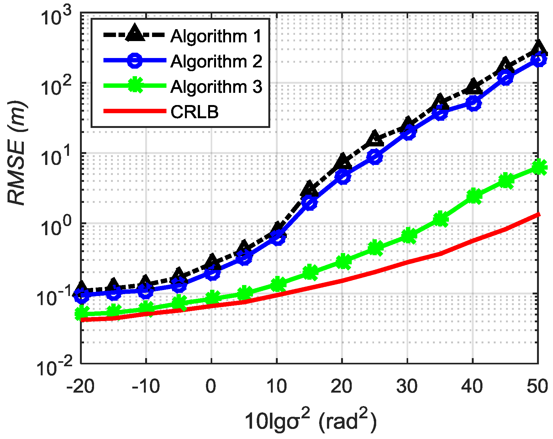
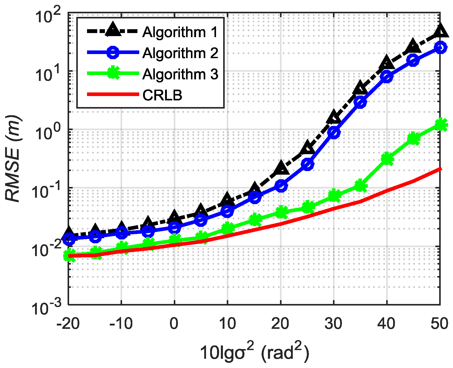
5.2. Algorithm Performance in Different Orientation Angle Measurement Error

We analyze how the positioning accuracy changes with the gain of orientation angle-measurement error. The number of nodes is five, and the SNR is fixed at 0 dB and 10 dB.

Experiment 1: When SNR = 10 dB, the RMSE changes with the orientation angle-measurement error through 5000 Monte Carlo simulations, as shown in Figure 3.

The single solid curve in Figure 3 is CRLB. The positioning accuracy of three algorithms is close to CRLB when the orientation angle-measurement error is small, and Algorithm 3 performs slightly better than Algorithm 1 and Algorithm 2. With the gain of the orientation angle-measurement error, the RMSE of Algorithm 1 and Algorithm 2 increase significantly, while Algorithm 3 continues to have a smaller RMSE. This shows that Algorithm 3 still possesses a high positioning accuracy with large errors, and the greater the error, the more obvious is the advantage.

Experiment 2: When SNR = 0 dB, the change in RMSE with the orientation angle-measurement error under the same conditions is shown in Figure 4.

Comparing Figure 4 with Figure 3, when the SNR is reduced, the three algorithms are still able to locate the target but with a declining accuracy. The comparison between algorithms shows that the positioning accuracy of Algorithm 3 is obviously better than Algorithms 1 and 2 when the orientation angle-measurement error increases, and the greater the error, the more obvious is the advantage. Simulations show that the proposed Algorithm 3 can still accurately estimate the target despite the large orientation angle-measurement error.

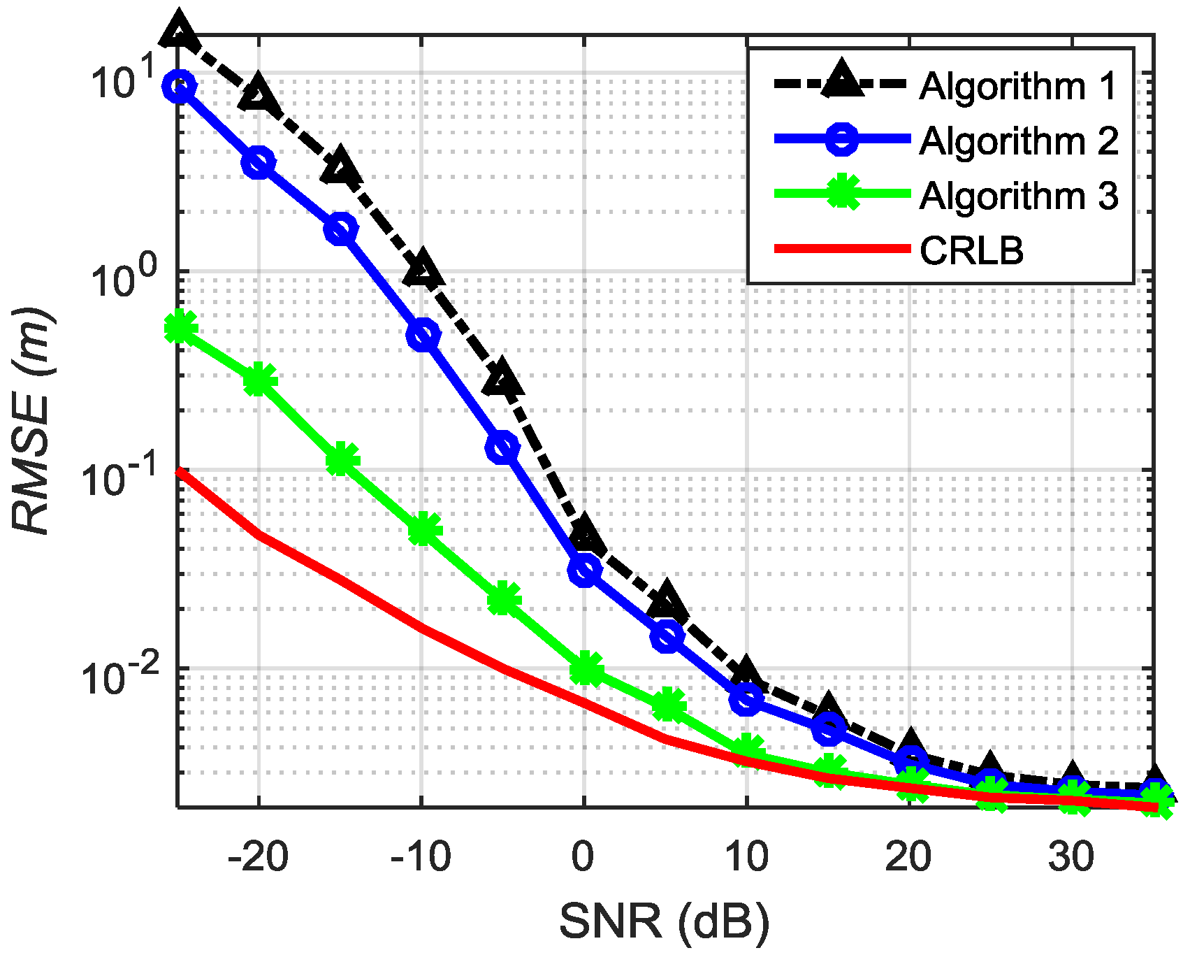
5.3. Performance for Varying SNR

To analyze the effect of gain in SNR on positioning accuracy when the orientation angle-measurement error is fixed, we change the SNR from −25 dB to 35 dB, the results of which are shown in Figure 5.

As is shown in Figure 5, when the SNR is low, the positioning results of all the three algorithms display a larger deviation, and even worse for Algorithms 1 and 2. With the increase in SNR, the positioning accuracy of all of the algorithms improves. Algorithm 3 approaches CRLB when the SNR reaches 10 dB, while Algorithms 1 and 2 do not approach CRLB until the SNR reach 25 dB. When the SNR is greater than 30 dB, all three algorithms exhibit similar targeting results. Simulations show that the proposed algorithm is more accurate than the traditional methods under low SNR conditions.

6. Conclusions

In this paper, we proposed a lateral cross localization algorithm using orientation angle. The algorithm can address targeting problems, such as poor resolution, low accuracy under large orientation-angle error, and background noise in near-field environments of traditional algorithms. We constructed the estimation prediction equations with the lateral cross positioning system geometry model and the numerical model. A progressive, unbiased estimate of the target was obtained via an iterative process control of the prediction equations. A large number of simulations verified that the proposed algorithm has a smaller location RMSE under different orientation-angle error values and SNR, and the proposed approach displays remarkable potential for engineering applications.

References

1. Zhang, L.; Gan, J.Q.; Wang, H. Localization of neural efficiency of the mathematically gifted brain through a feature subset selection method. Cogn. Neurodyn. 2015, 9, 495–508. [Google Scholar] [CrossRef] [PubMed]
2. Otero-Garcia, M.; Agustin-Pavon, C.; Lanuza, E.; Martínez-García, E. Distribution of oxytocin and co-localization with arginine vasopressin in the brain of mice. Brain Struct. Funct. 2015, 20. [Google Scholar] [CrossRef] [PubMed]
3. Bulychev, Y.G.; Bulychev, V.Y.; Ivakina, S.S.; Nasenkov, I.G. Complex Matching–Identification Method as Applied to Multiposition Angle-Measuring Systems of Passive Location Based on Invariants. J. Commun. Technol. Electron. 2015, 60, 762–772. [Google Scholar] [CrossRef]
4. Perrine-Walker, F.M.; Jublanc, E. The localization of auxin transporters PIN3 and LAX3 during lateral root development in Arabidopsis thaliana. Biol. Plant. 2014, 58, 778–782. [Google Scholar] [CrossRef]
5. Lobkova, L.M.; Golovin, V.V.; Troitsky, A.V. The Impact of Angle-of-Arrival Fluctuations of Electromagnetic Wave on the Direction of Maximum Radiation of Aperture Antennas. Radioelectron. Commun. Syst. 2008, 51, 150–155. [Google Scholar] [CrossRef]
6. Fu, Y.; Nistor, A.I. Constant Angle Property and Canonical Principal Directions for Surfaces in M2(c) × R1. Mediterr. J. Math. 2013, 10, 1035–1049. [Google Scholar] [CrossRef]
7. Zsedrovits, T.; Zarandy, A.; Vanek, B.; Peni, T.; Bokor, J.; Roska, T. Estimation of Relative Direction Angle of Distant, Approaching Airplane in Sense-and-Avoid. J. Intell. Robot Syst. 2013, 69, 407–415. [Google Scholar] [CrossRef] [Green Version]
8. Guillian, E.H. Far Field Monitoring of Rogue Nuclear Activity with an Array of Large Anti-neutrino Detectors. Earth Moon Planets 2006, 99, 309–330. [Google Scholar] [CrossRef]
9. Bulychev, Y.G.; Vernygora, V.N.; Mozol, A.A. The Direction-Finding Powered Method for Definition of Distance to Target, Using Two Measurements of Autonomous Angle-Measurement System. Radioelectron. Commun. Syst. 2009, 52, 606–612. [Google Scholar] [CrossRef]
10. Luo, Q.; Meng, Z.; Han, C. Solution algorithm of a quasi-Lambert’s problem with fixed flight-direction angle constraint. Celest. Mech. Dyn. Astr. 2011, 109, 409–427. [Google Scholar] [CrossRef]
11. Weiss, A.J. Direct position determination of narrowband radio frequency transmitters. IEEE Signal Process. Lett. 2004, 11, 513–516. [Google Scholar] [CrossRef]
12. Chen, J.C.; Hudson, R.E.; Yao, K. Maximum-likelihood source localization and unknown sensor location estimation for wideband signals in the near-field. IEEE Trans. Signal Process. 2002, 50, 1843–1854. [Google Scholar] [CrossRef]
13. Weiss, A.J.; Amar, A. Direct position determination of multiple radio signals. EURASIP J. Adv. Signal Process. 2005. [Google Scholar] [CrossRef]
14. Bakhti, S.; Destouches, N.; Tishchenko, A.V. Singular Representation of Plasmon Resonance Modes to Optimize the Near and Far Field Properties of Metal Nanoparticles. Plasmonics 2015, 10, 1391–1399. [Google Scholar] [CrossRef]
15. Dunn, R.J.K.; Zigic, S.; Shiell, G.R. Modelling the dispersion of treated wastewater in a shallow coastal wind-driven environment, Geographe Bay, Western Australia: implications for environmental management. Environ. Monit. Assess. 2014, 186, 6107–6125. [Google Scholar] [CrossRef] [PubMed]
16. Yan, K.; Liu, L.; Yao, N.; Liu, K.; Du, W.; Zhang, W.; Yan, W.; Wang, C.; Luo, X. Far-Field Super-Resolution Imaging of Nano-transparent Objects by Hyperlens with Plasmonic Resonant Cavity. Plasmonics 2016, 11, 475–481. [Google Scholar] [CrossRef]
17. Tounsi, R.; Markiewicz, E.; Haugou, G.; Chaari, F.; Zouari, B. Combined effects of the in-plane orientation angle and the loading angle on the dynamic enhancement of honeycombs under mixed shear-compression loading. Eur. Phys. J. Spec. Top. 2016, 225, 243–252. [Google Scholar] [CrossRef]
18. Girod, L.; Lukac, M.; Trifa, V.; Estrin, D. The design and implementation of a self-calibrating distributed acoustic sensing platform. In Proceedings of the 4th International Conference on Embedded Networked Sensor Systems, Boulder, CO, USA, 1–3 November 2006; pp. 71–84.
19. Yip, L.; Comanor, K.; Chen, J.; Hudson, R.E.; Yao, K.; Vandenberghe, L. Array processing for target DOA, localization, and classification based on AML and SVM algorithms in sensor networks. In Information Processing in Sensor Networks, Proceedings of the Second International Workshop IPSN 2003, Palo Alto, CA, USA, 22–23 April 2003; Springer-Verlag: Berlin/Heidelberg, Germany, 2003; pp. 269–284. [Google Scholar]
20. Yao, K.; Chen, J.C.; Hudson, R.E. Maximum-likelihood acoustic source localization: experimental results. In Proceedings of the IEEE International Conference on Acoustics, Speech, and Signal Processing (ICASSP), Orlando, FL, USA, 13–17 May 2002; Volume 3, pp. 2949–2952.
21. Allen, M.; Girod, L.; Newton, R.; Madden, S.; Blumstein, D.T.; Estrin, D. Voxnet: An interactive, rapidly-deployable acoustic monitoring platform. In Proceedings of International Conference on Information Processing in Sensor Networks (IPSN), St. Louis, MO, USA, 22–24 April 2008; pp. 371–382.
22. Kaplan, L.M.; Le, Q.; Molnar, N. Maximum likelihood methods for bearings-only target localization. In Proceedings of the IEEE International Conference on Acoustics, Speech, and Signal Processing (ICASSP), Salt Lake City, UT, USA, 7–11 May 2001; Volume 5, pp. 3001–3004.
23. Kaplan, L.M.; Le, Q. On exploiting propagation delays for passive target localization using bearings-only measurements. J. Frankl. Inst. 2005, 342, 193–211. [Google Scholar] [CrossRef]
24. Stansfield, R.G. Statistical theory of DF fixing. Electr. Eng.-Part IIIA J. Inst. Radio Commun. 1947, 94, 762–770. [Google Scholar]
25. Dogancay, K. Bearings-only target localization using total least squares. Signal Process. 2005, 85, 1695–1710. [Google Scholar] [CrossRef]
26. Chan, Y.T.; Rudnicki, S.W. Bearings-only and Doppler-bearing tracking using instrumental variables. IEEE Trans. Aerosp. Electr. Syst. 1992, 28, 1076–1083. [Google Scholar] [CrossRef]
27. Dogancay, K. Passive emitter localization using weighted instrumental variables. Signal Process. 2004, 84, 487–97. [Google Scholar] [CrossRef]
28. Zhang, Y.J.; Xu, G.Z. Bearings-only target motion analysis via instrumental variable estimation. IEEE Trans. Signal Process. 2010, 58, 5523–5533. [Google Scholar] [CrossRef]
29. Ho, K.C.; Chan, Y.T. An asymptotically unbiased estimator for bearings-only and Doppler-bearing target motion analysis. IEEE Trans. Signal Process. 2006, 54, 809–822. [Google Scholar] [CrossRef]
30. Gu, G. A novel power-bearing approach and asymptotically optimum estimator for target motion analysis. IEEE Trans. Signal Process. 2011, 59, 912–922. [Google Scholar] [CrossRef]
31. Vaghefi, R.M.; Gholami, M.R.; Strom, E.G. Bearing-only target localization with uncertainties in observer position. In Proceedings of International Symposium on Personal, Indoor and Mobile Radio Communications Workshops, Instanbul, Turkey, 26–30 September 2010; pp. 238–242.
32. Le Cadre, J.P.; Jaetffret, C. On the convergence of iterative methods for bearings-only tracking. IEEE Trans. Aerosp. Electron. Syst. 1999, 35, 801–818. [Google Scholar] [CrossRef]
33. Gavish, M.; Weiss, A.J. Performance analysis of bearing-only target location algorithms. IEEE Trans. Aerosp. Electron. Syst. 1992, 28, 817–828. [Google Scholar] [CrossRef]
34. Bishop, A.N.; Anderson, B.D.O.; Fidan, B.; Pathirana, P.N.; Mao, G. Bearing-only localization using geometrically constrained optimization. IEEE Trans. Aerosp. Electron. Syst. 2009, 45, 308–320. [Google Scholar] [CrossRef]
35. Serov, A.V.; Mamonov, I.A.; Kol’tsov, A.V. Angular Distributions of Reflected and Refracted Relativistic Electron Beams Crossing a Thin Planar Target at a Small Angle to Its Surface. J. Exp. Theor. Phys. 2015, 121, 572–577. [Google Scholar] [CrossRef]
36. Wolbrecht, E.; Gill, B.; Borth, R.; Canning, J.; Anderson, M.; Edwards, D. Hybrid Baseline Localization for Autonomous Underwater Vehicles. J. Intell. Robot. Syst. 2015, 78, 593–611. [Google Scholar] [CrossRef]
Figure 1. Schematic of lateral cross positioning.
Information 07 00040 g001
Figure 2. Schematic of orientation cross positioning.
Information 07 00040 g002
Figure 3. RMSE curve with orientation angle measurement error for different algorithms at SNR = 10 dB.
Information 07 00040 g003
Figure 4. RMSE curve change with the orientation angle-measurement error for different algorithms at SNR = 0 dB.
Information 07 00040 g004
Figure 5. RMSE change with SNR for different algorithms.
Information 07 00040 g005