A Novel Global Path Planning Method for Mobile Robots Based on Teaching-Learning-Based Optimization

Abstract

The Teaching-Learning-Based Optimization (TLBO) algorithm has been proposed in recent years. It is a new swarm intelligence optimization algorithm simulating the teaching-learning phenomenon of a classroom. In this paper, a novel global path planning method for mobile robots is presented, which is based on an improved TLBO algorithm called Nonlinear Inertia Weighted Teaching-Learning-Based Optimization (NIWTLBO) algorithm in our previous work. Firstly, the NIWTLBO algorithm is introduced. Then, a new map model of the path between start-point and goal-point is built by coordinate system transformation. Lastly, utilizing the NIWTLBO algorithm, the objective function of the path is optimized; thus, a global optimal path is obtained. The simulation experiment results show that the proposed method has a faster convergence rate and higher accuracy in searching for the path than the basic TLBO and some other algorithms as well, and it can effectively solve the optimization problem for mobile robot global path planning.

1. Introduction

Path planning is to find the optimal path from the start to the goal in the workspace according to the optimization criterion (such as the lowest cost, the minimum time, the shortest length, etc.). The mobile robot path planning technology is an important branch in the field of intelligent mobile robot research. So far, there have been a large number of research results in this field. According to the robot’s knowledge about the environment, path planning can be divided into global path planning, in which the environmental information is completely known, and local path planning, in which the environmental information is completely unknown or partially unknown. At present, path planning methods commonly include: grid method [1], ant colony algorithm [2], artificial potential field method [3], neural network method [4], genetic algorithm(GA) [5], Artificial Bee Colony (ABC) algorithm [6,7], Differential Evolution(DE) algorithm [8], and particle swarm optimization (PSO) [9,10], etc. These methods may have their own advantages, but there also exist some weaknesses [11], such as poor adaptability for path map, high computational complexity, long search time, low convergence accuracy and easily trapping in the local optimum. So, to some extent, it makes the ability of path planning for mobile robots limited.

In recent years, the teaching-learning-based optimization (TLBO) algorithm has been proposed by Rao et al. [12,13]. This algorithm is very suitable to solve the path optimization problem due to its fast convergence speed and high precision. Therefore, it provides a new solution for the mobile robot’s global path planning. The TLBO requires only the common control parameters like population size and number of generations and does not require any algorithm-specific control parameters. It is an algorithm-specific parameter-less algorithm [14]. So, in the TLBO algorithm, there is no burden of tuning control parameters. Hence, the TLBO algorithm is simpler, more effective and involves relatively less computational cost. Therefore, the TLBO has been successfully applied in diverse optimization fields such as task scheduling, production planning and control, mechanical engineering, vehicle-routing problems in transportation, etc. Recently, several variants of the TLBO have been proposed to improve the performance. Rao et al. presented an elitist TLBO (ETLBO) algorithm [14] to solve complex constrained optimization problems, and used a modified version of TLBO algorithm [15] to solve the multi-objective optimization problem of heat exchangers. Furthermore, some modified TLBO algorithms have been proposed to solve the global function optimization problem [16,17,18,19] and the multi-objective optimization problem [15,20,21]. However, so far, applying the TLBO algorithm to solve the optimization problem for the mobile robot’s global path planning has not been reported in the literature. In our recent work, we have proposed a novel improved TLBO, which is called Nonlinear Inertia Weighted TLBO (NIWTLBO) [22]. In this paper, we apply this NIWTLBO algorithm to solve the optimization problem for the mobile robot’s global path planning.

The rest of this paper is organized as follows. In Section 2, the NIWTLBO algorithm is introduced. Section 3 describes the modeling method of the mobile robot’s path in static environment. In Section 4, the global path planning for the mobile robot is implemented by utilizing NIWTLBO algorithm. And Section 5 provides experimental results and performance analysis. Finally, our conclusions are mentioned in Section 6.

2. NIWTLBO Algorithm

In our recent work, we proposed a novel improved TLBO according to the learning and memory mechanism, which is called the NIWTLBO algorithm. This algorithm introduces a nonlinear inertia weighted factor into the basic TLBO to control the memory rate of learners, and used a dynamic inertia weighted factor to replace the original random number in the teacher phase and learner phase. We call the nonlinear inertia weighted factor as learning memory rate. As this is done, the NIWTLBO has not only faster convergence speed but also higher calculation accuracy for most of these optimization problems compared to the basic TLBO. The details of this algorithm can be referenced in our previous work [22].

2.1. Initialization

In this paper, NP denotes the number of learners in a class, D denotes number of subjects offered to the learners (i.e., dimensions of design variables), and MAXITER denotes maximum number of allowable iterations. The learners are randomly initialized randomly by a search space bounded by NP × D matrix using the equation as follows

$$X_{0,k,j}=L_j+rand\times \left(U_j-L_j\right), k=1,2,\cdots ,NP, j=1,2,\cdots ,D$$

(1)

where U_j and L_j represent the upper bound and lower bound of design variable, respectively.

2.2. Teacher and Learner Phase

We let $M_{i,j}=\frac{1}{NP}({\displaystyle \sum _{k=1}^{NP}}{X}_{i,k,j})$ be the mean result of the learners on a particular subject “j”, $X_{i,k,j}$ be the result of the jth subject offered to the kth learner at the ith iterator, and $X_{i,teacher}$ be the teacher at any iteration i.

In the teacher phase, the new set of improved learners can be expressed by using equation

$$X_{i,k,j}^{new}=w{X}_{i,k,j}^{old}+r_i^{\prime }(X_{i,teacher,j}-T_F{M}_{i,j})$$

(2)

$$T_F=round\left[1+rand\left(0,1\right)\left\{1-2\right\}\right]$$

(3)

$$w=1-exp\left(\frac{-ite{r}^2}{2\times {(MAXITER/8)}^2}\right)\times (1-w_{min})$$

(4)

$$r_i^{\prime }=0.5+\frac{rand(0,1)}{2}$$

(5)

where $w$ is the nonlinear inertia weighted factor; iter is the current iteration number; $w_{min}$ is the minimum value of the $w$, whose value should be in the range [0.5, 1] (Here it is selected 0.6); $r_i^{\prime }$ is the dynamic inertia weighted factor whose value is in the range [0.5, 1].

In the learner phase, the new set of improved learners can be expressed by using equation

$$X_{i,k,j}^{new}=\{\begin{array}{cc}w{X}_{i,k,j}^{old}+r_i^{\prime }\left(X_{i,k,j}-X_{i,q,j}\right)\hfill & \hfill \mathrm{if} f\left(X_{i,total\_k}\right)<f\left(X_{i,total\_q}\right),\\ w{X}_{i,k,j}^{old}+r_i^{\prime }\left(X_{i,q,j}-X_{i,k,j}\right)\hfill & \hfill otherwise\end{array}$$

(6)

where $X_{i,total\_k}$ and $X_{i,total\_q}$ represent the total result of the kth student and the qth student at the iteration i, respectively.

In every iteration, $X_{i,k,j}^{new}$ is the updated value of $X_{i,k,j}^{old}$. If the new value gives a better function value, then the old value is updated with the new value. The updated formula is given as

$$X_{i,k,j}^{old}=X_{i,k,j}^{new}, \mathrm{if} f\left(X_{i,total\_k}^{new}\right)<f\left(X_{i,total\_k}^{old}\right)$$

(7)

where $X_{i,total\_k}^{new}$ and $X_{i,total\_k}^{old}$ represent the new and old total result of the kth student at the iteration i for all subjects, respectively. Here, $X_{i,total\_k}^{old}={\displaystyle \sum _{j=1}^D{X}_{i,k,j}^{old}}$.

In this modified TLBO, the individuals try to sample diverse zones of the search space during the early stages of the search. During the later stages, the individuals adjust the movements of trial solutions finely so that they can explore the interior of a relative small space. The NIWTLBO increases the probability of stochastic variations and enlarges the difference value added to the existing learners, so as to improve population diversity, avoid prematurity in the search process and increase the ability of the basic TLBO to escape from the local optima.

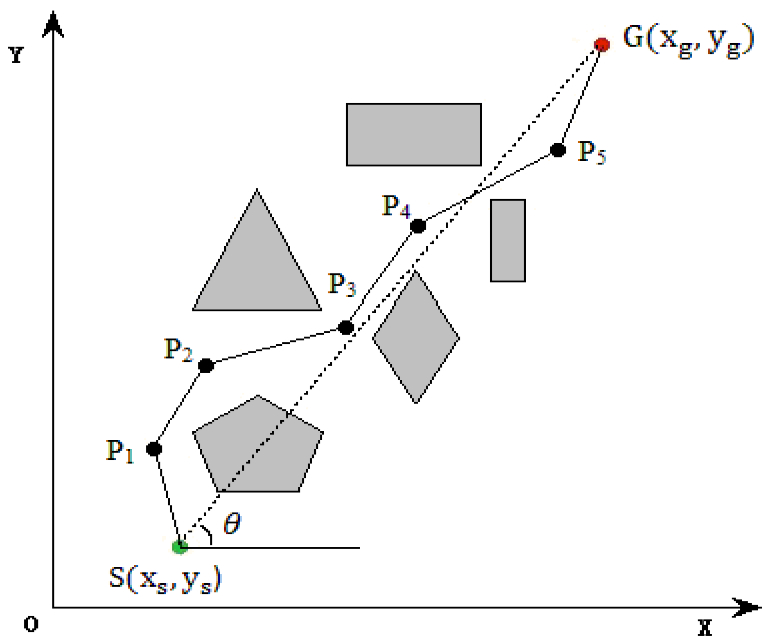
3. Mobile Robot Path Modeling

As the design model of TLBO algorithm is very suitable to solve the continuous space optimization problems, therefore, the NIWTLBO algorithm can effectively solve the robot global path planning problems similarly. Here, we use the 2D coordinate in continuous space to express the environment of robot movement. In the simulation environment model, the obstacles can be described as the approximate geometric shapes, such as the circular objects and convex polygon objects in Figure 1 (the approximate concave polygon object can be divided into multiple convex polygons).

In order to describe the robot global path planning problem, it is necessary to design the movement environment of the robot firstly. We assume the environment as the following: (1) robot movement is limited in 2D space; (2) the space exists several known static obstacles, which are distributed in different position. The obstacles are expressed by the convex polygon and circle whose position and size are known; (3) considering the size of the robot itself, the radius of obstacles is expanded according to the size of the robot, so the robot may be considered as a mass point. The purpose of this paper is using the proposed algorithm to find a shortest path from a starting point to goal point without colliding with collision obstacles in the known static environment. As shown in Figure 2, in the coordinate system XOY of motion environment map, gray solid objects represent obstacles. $S(x_s,y_s)$ is the starting point, and $G(x_g,y_g)$ is the goal point. The path planning goal is to find a point set $P=\left\{S,P_1,\cdots ,P_i,\cdots ,P_d,G\right\}$ in global search space so that we can obtain the shortest path from the starting point to the goal point, on the premise that the line between any two adjacent points does not pass through the obstacles.

In order to simplify the computational complexity of the proposed algorithm, it is necessary to transform the original environment’s coordinate system into a new one. The starting point is considered as the origin, and the line segment SG between the starting point and the goal point is considered as Y axis in a new environment coordinate ${\mathrm{X}}^{\prime }{\mathrm{O}}^{\prime }{\mathrm{Y}}^{\prime }$ showing in Figure 2. θ is the angle between SG and X axis in the original coordinate XOY. The original coordinate XOY is translated to $(x_s,y_s)$ and then rotated $\frac{\pi }{2}-\theta$ degrees clockwise, thus a new coordinate ${\mathrm{X}}^{\prime }{\mathrm{O}}^{\prime }{\mathrm{Y}}^{\prime }$ is obtained. The formula of the coordinate transformation is as follows:

$$\left[\begin{array}{l}{x}^{\prime }\\ y^{\prime }\end{array}\right]=[\begin{array}{l}\cos \left(\frac{\pi }{2}-\theta \right)\\ \sin \left(\frac{\pi }{2}-\theta \right)\end{array} \begin{array}{l}-\sin \left(\frac{\pi }{2}-\theta \right)\\ \cos \left(\frac{\pi }{2}-\theta \right)\end{array}]\cdot \left(\begin{array}{l}x\\ y\end{array}\right)+\left[\begin{array}{l}{x}_s\\ y_s\end{array}\right]$$

(8)

In Figure 2, the line segment SG from the starting point to goal point is equally divided into d +1 segments (such as d = 9 in the Figure 2). Drawing lines perpendicular to the $Y^{\prime }$ axis through each division point, we pick any one of the points on each line from the starting point to the goal point to form a set of path points in order. Due to the path points on the vertical coordinate being equidistant, the vector $X=\left\{x_s,x_1,x_2,\cdots ,x_d,x_g\right\}$ formed by the horizontal ordinate of the path points (i.e., P_i) can express one workable path. Because the coordinates of starting point and goal point are known, the above path can be simplified as $X=\left\{x_1,x_2,\cdots ,x_d\right\}$. Therefore, the path planning problem can be converted into searching the horizontal ordinate x_i of a path point on each equidistant line, which ensures that the path connecting the points $X=\left\{x_s,x_1,x_2,\cdots ,x_d,x_g\right\}$ in sequence is shortest with avoiding obstacles.

4. Implementation of Path Planning Based on NIWTLBO Algorithm

The path planning problem in static environment with obstacles is actually a constrained optimization problem without collision. In this section, we apply the NIWTLBO algorithm to solve the constrained optimization problem for the mobile robot’s path planning.

4.1. Initialization

First, we need to define the number of students (i.e., population size), the number of subjects for learners (i.e., number of decision variables, here is the number of the path points P_i), and the maximum generations. Then, the decision variables of the population are initialized by a set of random values (i.e., the x-coordinate of the path points P_i) within the boundary of the path map, which are equivalent to the marks of the subjects for students. Meanwhile, in order to ensure all path points in the area where the obstacles do not exist, it is necessary to deal with the obstacle constraints for a workable path in initial population. The obstacle constraints are discussed in Section 4.3.

4.2. Individual Fitness Function

Path planning of the mobile robot in a static environment should be satisfied with the shortest length of the path and avoid static obstacles. The main issue of this section is to solve the shortest path problem under obstacle constraints. Under the conditions of an existing collision-free path, it is important that the path length as short as possible. Therefore, we choose the path length function as an individual fitness function to evaluate the merits of the path. We assume that the starting point of the mobile robot is $\mathrm{S}(x_0,y_0)$ and the goal point is $\mathrm{G}(x_{d+1},y_{d+1})$. Due to the equal distance between the vertical lines across Y axis, the path is represented as $x=\left\{x_0,x_1,\cdots ,x_i,\cdots ,x_d,x_{d+1}\right\}$, x_i is the horizontal ordinate of the path point P_i as shown in Figure 2. Therefore, the length of the path can be defined as

$$f={\displaystyle \sum }_{i=0}^d\sqrt{{\left(x_{i+1}-x_i\right)}^2+{\left(y_{i+1}-y_i\right)}^2}={\displaystyle \sum }_{i=0}^d\sqrt{{\left(x_{i+1}-x_i\right)}^2+{\left(\frac{y_{d+1}-y_0}{d+1}\right)}^2}$$

(9)

Thus, the optimization problem of this paper is solving the shortest length of the workable path under obstacle constraints, i.e., solving the value of min(f(x)).

4.3. Obstacle Constraints

In the path planning problem, obstacle constraints mainly have two aspects: one is the boundary of the path map; the other is the obstacle avoidance. The x-coordinate (i.e., x_i) of the path point P_i cannot exceed the specified upper and lower bounds, meanwhile the position of these points cannot be in the obstacle region. If the x_i is beyond the boundary, a new x_i value is selected randomly again. If the position of a path point is in an obstacle region, it must be re-located in the bound range in the positive or negative direction of x_i until a new position is found that is not in the obstacle region. Thus, the x-coordinate of the path point can be limited between the upper and lower bounds, and be excluded from the obstacle region.

Aside from ensuring the path point position does not exceed the effective boundary range, we should also consider whether the obstacles are on the line between two adjacent path points. If there is one obstacle on the line, the path would be invalid. It is necessary to repeat the search for a new path point. Therefore, we must detect the availability of a path between two adjacent path points in each generation of the population. For any one path $x=\left\{x_1,x_2,\cdots ,x_i,x_{i+1},\cdots ,x_d\right\}$, if the line between x_i and x_i+1 is intersect with obstacles, it is necessary to re-select x_i+1. If the valid x_i+1 is still not found after trying a certain number of times, the x_i should be re-selected until a path point is found according to the constraint condition.

4.4. The Step of NIWTLBO Algorithm

The steps for solving the problem of the mobile robot path planning are as follows:

Step1:

Initialize NP (number of learners), D (number of subject dimensions) and MAXITER (number of generations).

Step2:

Initialize the learners X according to Equation (1) and ensure the marks of learners are limited in the range of the x-coordinate of the map, then according to Equation (9), calculate the initial value of the fitness function f(x) (i.e., the length of a path) to evaluate all learners X.

Step3:

Calculate the nonlinear inertia weighted parameter w and the dynamic inertia weighted factor $r_i^{\prime }$ according to Equations (4) and (5), respectively.

Step4:

Choose the best learner to be the teacher of the current generation, and calculate the mean result of each subject.

Step5:

Learners are learning from the teacher. Calculate the new marks of learners according to Equation (2) and ensure the marks are limited in the range of the x-coordinate of the map, evaluate all learners by calculating the fitness value of individuals (i.e., the length of a path). During the teacher phase, update all individuals according to Equation (7), and pass all accepted individuals to the learner phase.

Step6:

Execute the learner phase. Re-calculate the new marks of learners according to Equation (6) and the fitness value of individuals (i.e., the length of a path), update all individuals according to Equation (7) in the same way. The accepted individuals are passed to the next iteration.

Step7:

Check the repeated solutions. If there are repeated solutions, generate new individuals for the repeated solutions by the mutation operator.

Step8:

If the stopping condition is satisfied, terminate the algorithm and output the best solution. Otherwise, go to Step 3.

5. Experimental Results and Analysis

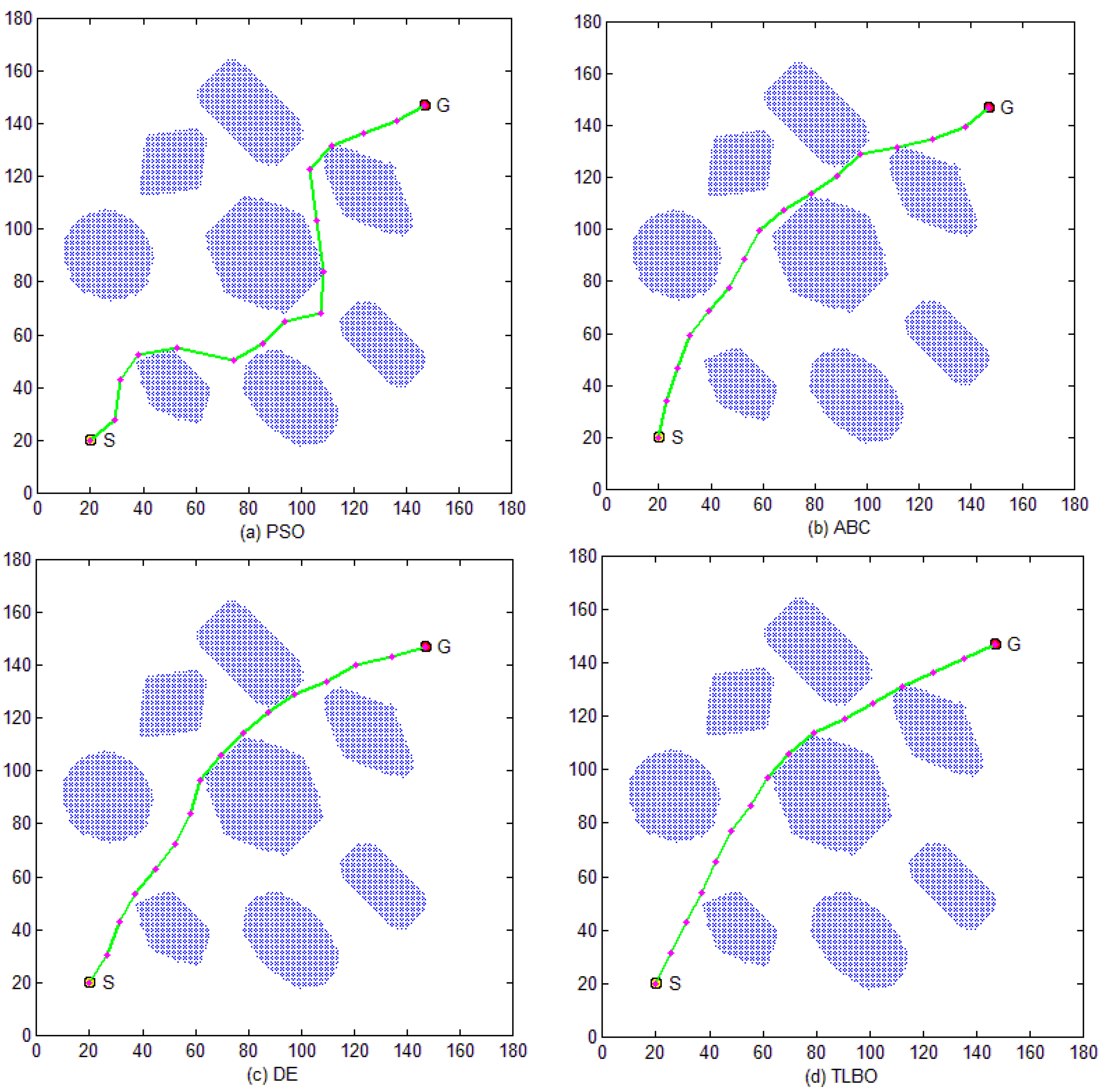
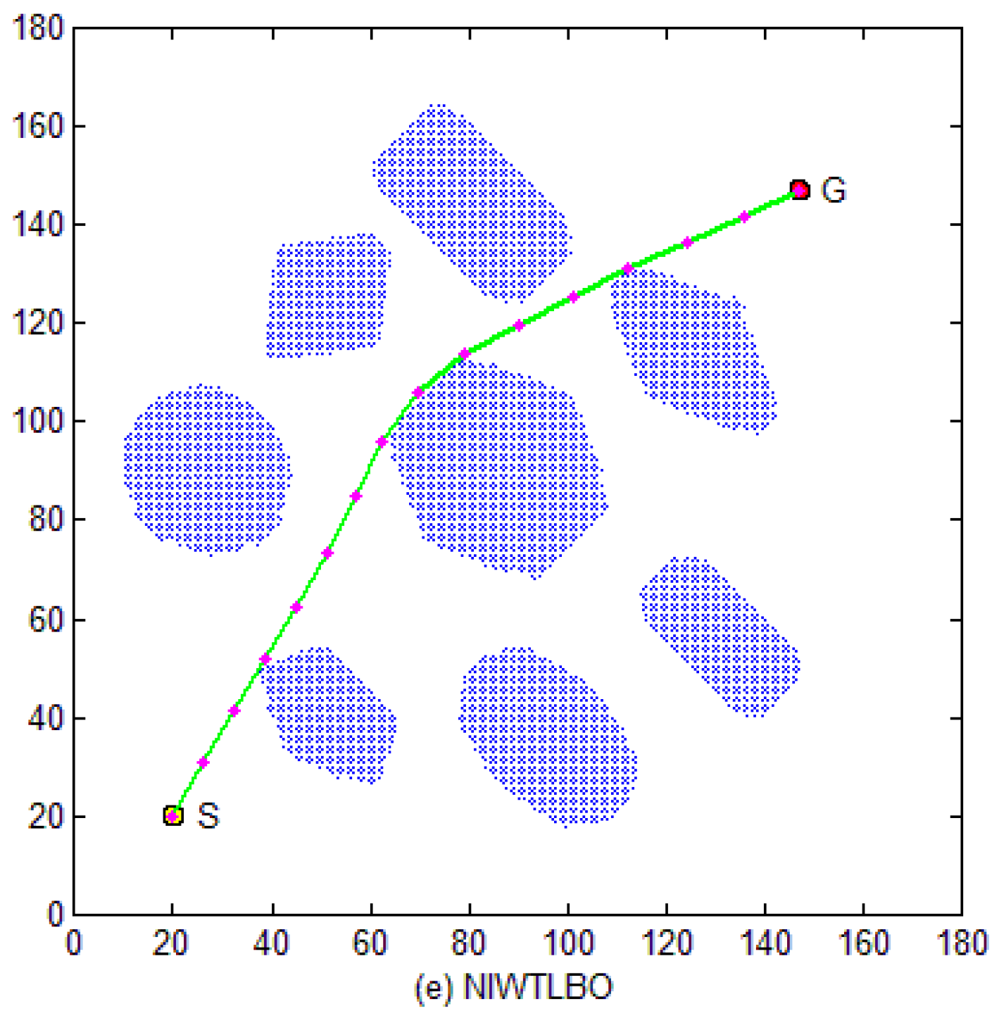
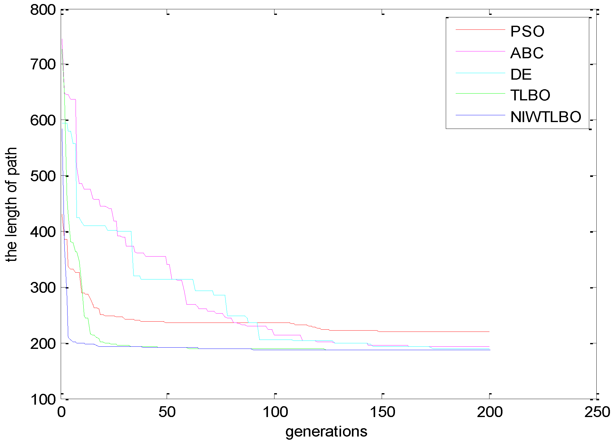
5.1. NIWTLBO vs. PSO, ABC, DE and TLBO

In this experiment, the size of the movement environment map of the mobile robot is 180 × 180 pixels, the coordinates of start point and goal point are (20, 20) and (147, 147), respectively. To be fair, the standard particle swarm optimization (PSO) algorithm, artificial bee colony (ABC) algorithm, differential evolution (DE) algorithm, the basic TLBO algorithm, and the proposed NIWTLBO algorithm are simulated in the same environment. That is, in all algorithms, the number of learners (i.e., NP) is set to 20, the number of subject dimensions (i.e., D) is set to 14, and the max number of iterations (i.e., MAXITER) is set to 200. In the PSO, C1 = C2 = 2.0, Inertia weight w = 0.9; for the ABC there are no such other specific parameters to set; in the DE, F is a real constant which affects the differential variation between two Solutions and R is crossover rate. Set F = 0.5, R = 0.4; for the TLBO and NIWTLBO, there are no parameters to set either. The results of all algorithms, in the form of mean solution and standard deviation, are obtained in 30 independent runs on the path fitness function. The comparative results of the path length are recorded in

Table 1. Comparative results of path length.

Algorithm	Min. Value	Max. Value	Mean	Std
PSO	219.022	240.573	228.434	8.0535
ABC	190.083	211.559	192.654	7.9538
DE	189.811	210.876	191.326	7.8426
TLBO	187.484	199.641	188.043	5.1192
NIWTLBO	186.988	190.648	187.621	1.6746

. The optimal path maps of each algorithm are shown as Figure 3. The Figure 4 shows the optimal convergence graph for all algorithms.

It is observed from the results in Table 1 and Figure 3 that the path of PSO is the worst, and the paths of TLBO and NIWTLBO are better. The convergence rate of the PSO, TLBO and NIWTLBO is faster. At the same time, the NIWTLBO can improve the search accuracy and achieve the optimal path ideally. The PSO has a poor local search ability because it could not find the better path after some certain generations. The particles so easily veer from the feasible region to the infeasible region in the search process in the PSO algorithm, which leads to large number particles changing their optimal search direction after the constraint processing. So the final result is unsatisfactory. The convergence rate of the ABC is slower, and it easily becomes trapped in a local optimal solution due to its poor ability of exploration. The DE algorithm is similar to the ABC. The ABC and the DE algorithms may achieve ideal path after over 2000 generations, which need more run time. However, the NIWTLBO algorithm can obtain the better optimal path after fewer generations. From Figure 4, we can see clearly that the NIWTLBO algorithm had the fastest convergence rate and performs better than the basic TLBO, PSO, ABC and DE algorithms.

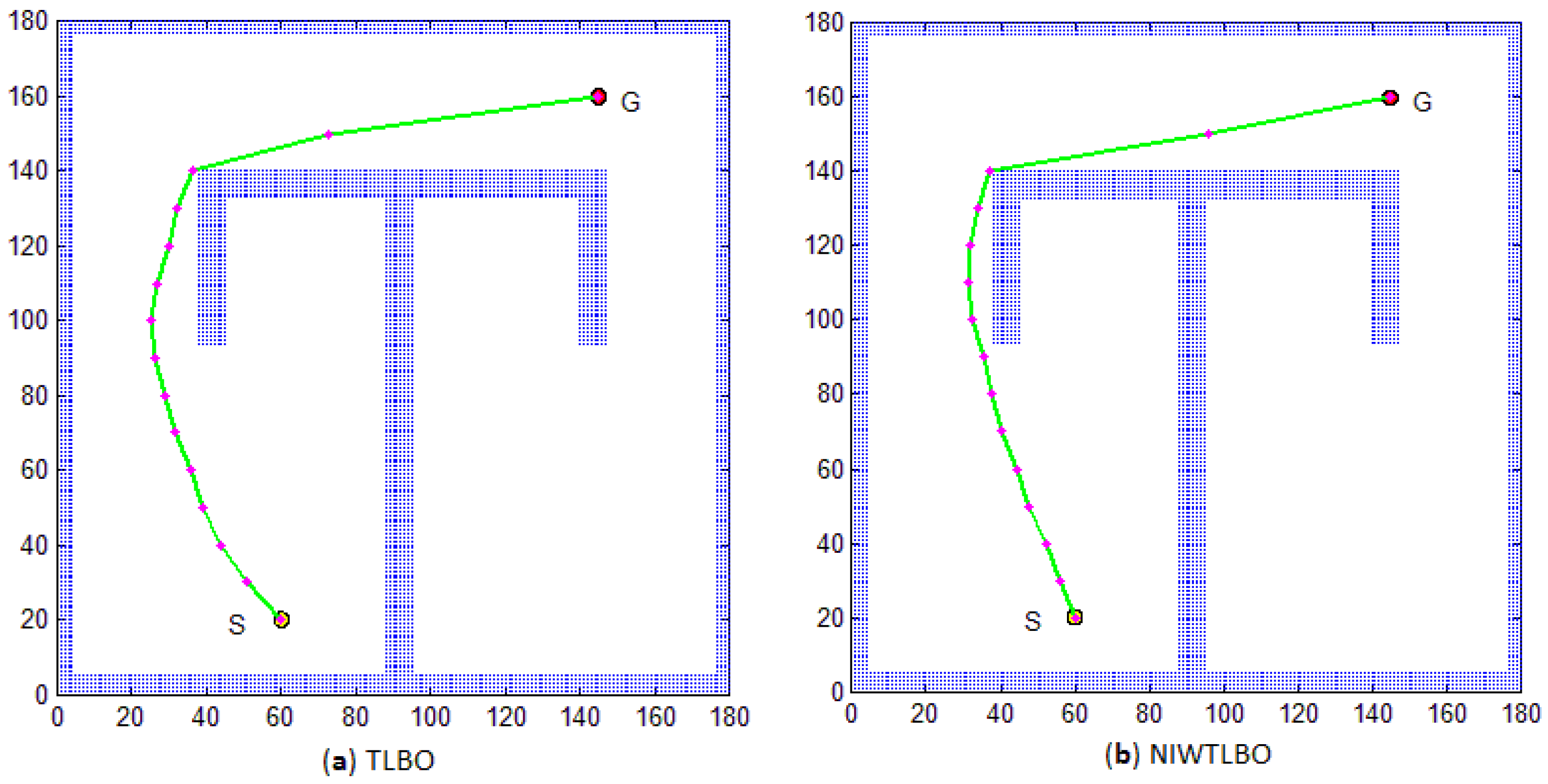
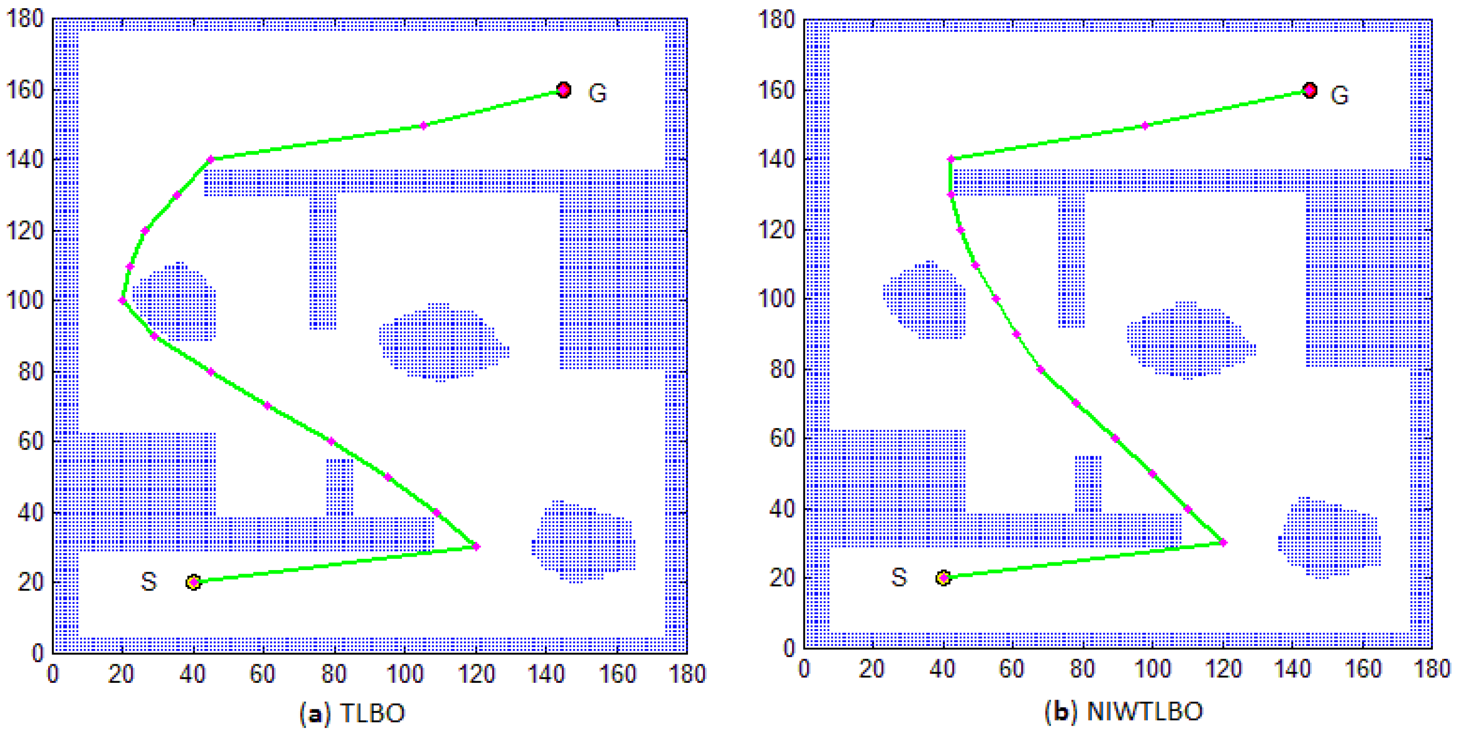
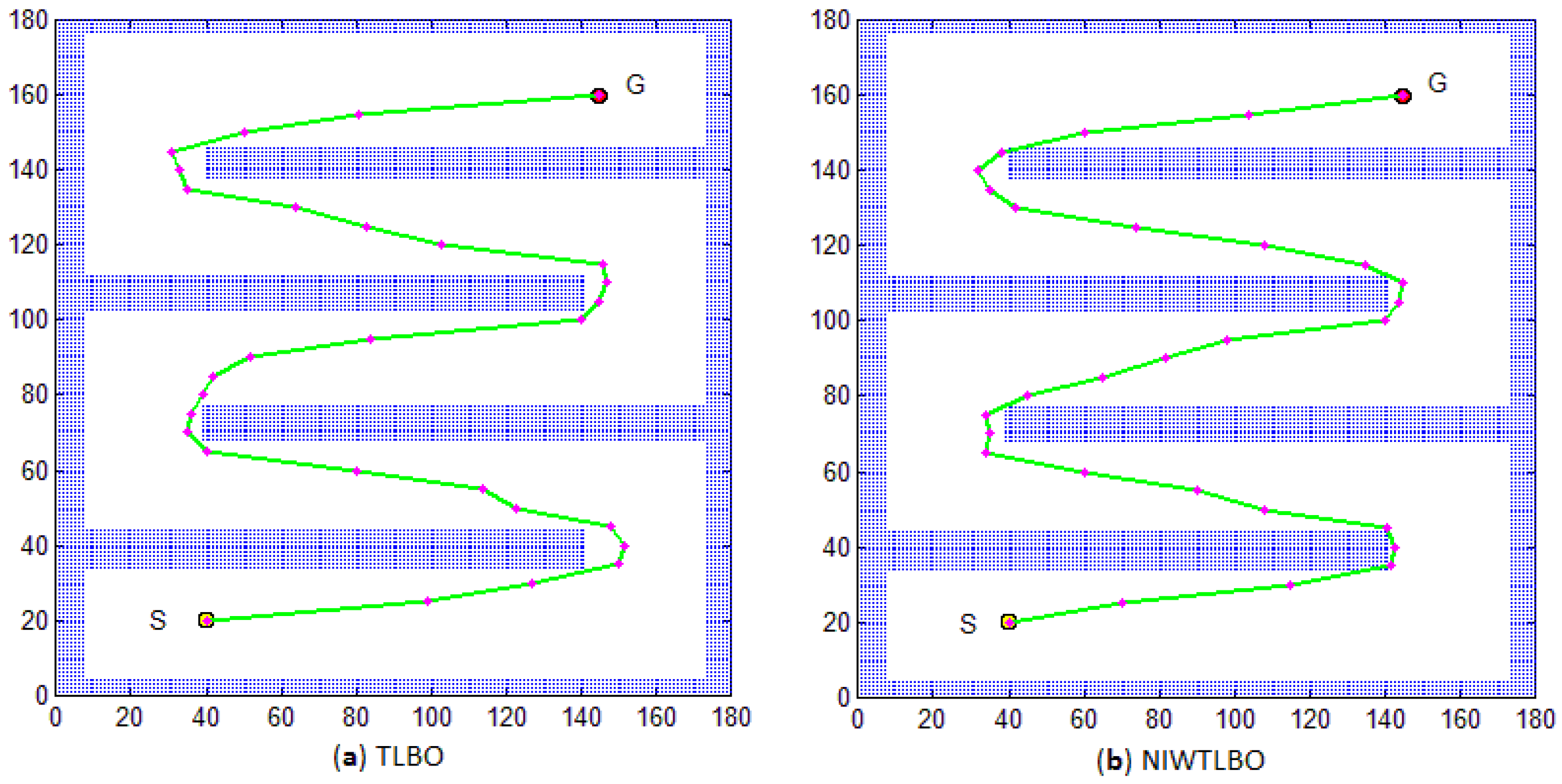
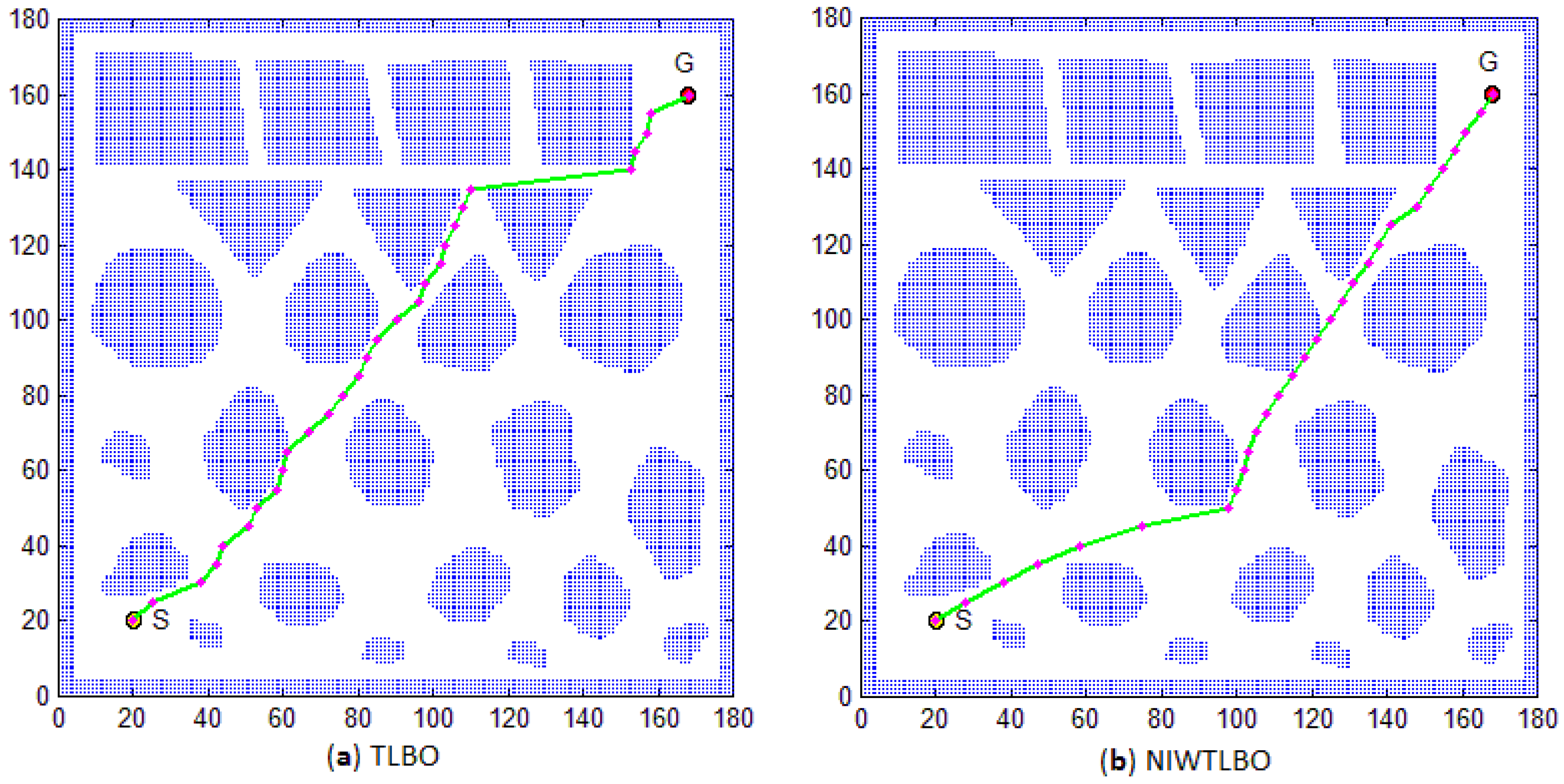
5.2. NIWTLBO vs. TLBO in Different Scenarios of the Path Planning with No Coordinate Transformation

In order to gain more insight about the usefulness of the proposed method, the different scenarios of the path planning are used in our experiments. We use several scenarios in the path planning dataset [23] which is the repository at the Czech Technical University to prove the ability of path planning. The motion planning maps are resized to 180 × 180 pixels. In order to simplify the processing, we do not rotate the coordinate of the maps in these experiments. For the start point $S(x_s,y_s)$ and the goal point $G(x_g,y_g)$, the difference $\Delta y=(y_g-y_s)$ is equally divided into D + 1 segments. Drawing the lines paralleling to the x-axis through each division point, we can get the $y_i$ coordinate of each path point, which is a constant value. Thereby, the optimization method is the same as the original. We only need to select the $x_i$ on each parallel line for optimization. This method is more suitable for the motion planning maps expressed by the images. In the experiments, the number of learners (i.e., NP) is set to 25, and the max number of iterations (i.e., MAXITER) is set to 300. The NIWTLBO and the basic TLBO algorithms are executed 10 times in each motion planning map, respectively. The best results of every scenario for the algorithms are shown in Figure 5, Figure 6, Figure 7 and Figure 8.

After 10 experiments for each motion planning map, we have achieved the optimal path. From Figure 5 to Figure 8, we can observe that the NIWTLBO method performs better than the basic TLBO on the path planning. Due to the weak ability of exploration and escaping from the local optima, the path obtained by the basic TLBO is not the shortest. The NIWTLBO method improves the population diversity with higher probability of stochastic variations, and it is not easy to trap into the local optima. Therefore, it can achieve the better results.

However, the proposed path planning model has some limitations. When the motion planning map only contains the “N” type path, or when the motion planning map is the scenario of rooms, the path planning may fail to find the valid path. We will improve this path planning model and the code of the proposed algorithm to solve such problems in future work.

6. Conclusions

TLBO is a new swarm intelligence optimization algorithm that can better solve the continuous space optimization problem. The algorithm is simple and parameter-less with fast convergence speed and high search accuracy. In our recent work, an improved TLBO algorithm called NIWTLBO algorithm is proposed. We apply this algorithm to the global path planning problem of mobile robots in this paper. The simulation experiments show that the algorithm has obvious advantages for the optimization problem of the robot’s global path planning, compared with PSO, ABC, DE and the basic TLBO algorithm. It can obtain the optimal path with fewer generations and shorter path length than the other algorithms. During the early stages of the search in the NIWTLBO, the individuals try to sample diverse zones of the search space. They adjust the movements of trial solutions finely so that they can explore the interior of a relative small space during the later stages. Therefore, it has stronger ability in terms of exploration and escaping from the local optima. Thereby, the NIWTLBO can achieve the acceptable performance for mobile robot global path planning.

In future work, the proposed algorithm will be improved and used to solve the dynamic local path planning problem of mobile robots combined with the rolling window method, and it will be extended to solve more complex functions and multi-objective optimization problems.

References

1. Châari, I.; Koubâa, A.; Bennaceur, H.; Ammar, A.; Trigui, S.; Tounsi, M.; Shakshuki, E.; Youssef, H. On the Adequacy of Tabu Search for Global Robot Path Planning Problem in Grid Environments. Proced. Comput. Sci. 2014, 32, 604–613. [Google Scholar] [CrossRef]
2. Garcia, M.A.P.; Montiel, O.; Castillo, O.; Sepúlveda, R.; Melin, P. Path planning for autonomous mobile robot navigation with ant colony optimization and fuzzy cost function evaluation. Appl. Soft Comput. 2009, 9, 1102–1110. [Google Scholar] [CrossRef]
3. Yin, L.; Yin, Y.X. Simulation Research on Path Planning Based on Dynamic Artificial Potential Field. J. Syst. Simul. 2009, 21, 3325–3320. [Google Scholar]
4. Kumar, M.P.S.; Rajasekaran, S. A neural network based path planning algorithm for extinguishing forest fires. Int. J. Comput. Sci. Issues 2012, 9, 563–568. [Google Scholar]
5. Tuncer, A.; Yildirim, M. Dynamic path planning of mobile robots with improved genetic algorithm. Comput. Electr. Eng. 2012, 38, 1564–1572. [Google Scholar] [CrossRef]
6. Liang, J.-H.; Lee, C.-H. Efficient collision-free path-planning of multiple mobile robots system using efficient artificial bee colony algorithm. Adv. Eng. Softw. 2015, 79, 47–56. [Google Scholar] [CrossRef]
7. Contreras-Cruz, M.A.; Ayala-Ramirez, V.; Hernandez-Belmonte, U.H. Mobile robot path planning using artificial bee colony and evolutionary programming. Appl. Soft Comput. 2015, 30, 319–328. [Google Scholar] [CrossRef]
8. Das, S.; Abraham, A.; Chakraborty, U.K.; Konar, A. Differential Evolution Using a Neighborhood-Based Mutation Operator. IEEE Trans. Evolut. Comput. 2009, 13, 526–553. [Google Scholar] [CrossRef]
9. Beheshti, Z.; Shamsuddin, S.M. Non-parametric particle swarm optimization for global optimization. Appl. Soft Comput. 2015, 28, 345–359. [Google Scholar] [CrossRef]
10. Bo, S.; Dong, C.W.; Geng, X.Y. Particle Swarm Optimization Based Global Path Planning for Mobile Robots. Control Decis. 2005, 20, 1052–1054. [Google Scholar]
11. Henrich, D. Fast Motion Planning by Parallel Processing—A Review. Intell. Robot. Syst. 1997, 20, 45–69. [Google Scholar] [CrossRef]
12. Rao, R.V.; Savsani, V.J.; Vakharia, D.P. Teaching-learning-based optimization: A novel method for constrained mechanical design optimization problems. Comput. Aided Des. 2011, 43, 303–315. [Google Scholar] [CrossRef]
13. Rao, R.V.; Savsani, V.J.; Vakharia, D.P. Teaching-Learning-Based Optimization: An optimization method for continuous non-linear large scale problems. Inf. Sci. 2012, 183, 1–15. [Google Scholar] [CrossRef]
14. Rao, R.V.; Patel, V. An elitist teaching-learning-based optimization algorithm for solving complex constrained optimization problems. Int. J. Ind. Eng. Comput. 2012, 3, 535–560. [Google Scholar] [CrossRef]
15. Rao, R.V.; Patel, V. Multi-objective optimization of heat exchangers using a modified teaching-learning-based optimization algorithm. Appl. Math. Model. 2013, 37, 1147–1162. [Google Scholar] [CrossRef]
16. Satapathy, S.C. Weighted Teaching-Learning-Based Optimization for Global Function Optimization. Appl. Math. 2013, 4, 429–439. [Google Scholar] [CrossRef]
17. Chen, D.; Zou, F.; Li, Z.; Wang, J.; Li, S. An improved teaching-learning-based optimization algorithm for solving global optimization problem. Inf. Sci. 2015, 297, 171–190. [Google Scholar] [CrossRef]
18. Satapathy, S.C. Improved teaching learning based optimization for global function optimization. Decis. Sci. Lett. 2013, 2, 23–34. [Google Scholar] [CrossRef]
19. Rao, R.V.; Patel, V. An improved teaching-learning-based optimization algorithm for solving unconstrained optimization problems. Sci. Iran. 2013, 20, 710–720. [Google Scholar] [CrossRef]
20. Sultana, S.; Roy, P.K. Multi-objective quasi-oppositional teaching learning based optimization for optimal location of distributed generator in radial distribution systems. Int. J. Electr. Power Energy Syst. 2014, 63, 534–545. [Google Scholar] [CrossRef]
21. Rao, R.V.; Patel, V. A multi-objective improved teaching-learning based optimization algorithm for unconstrained and constrained optimization problems. Int. J. Ind. Eng. Comput. 2014, 5, 1–22. [Google Scholar]
22. Wu, Z.S.; Fu, W.P.; Xue, R. Nonlinear Inertia Weighted Teaching-Learning-Based Optimization for Solving Global Optimization Problem. Comput. Intell. Neurosci. 2015, 2015, 1–15. [Google Scholar] [CrossRef] [PubMed]
23. Motion Planning Maps. Available online: http://imr.ciirc.cvut.cz/planning/maps.xml (accessed on 4 July 2016).
Figure 1. The path map of mobile robot movement environment.
Information 07 00039 g001
Figure 2. The new path map after coordinate transformation.
Information 07 00039 g002
Figure 3. The optimal path map of the different algorithms. (a) The result of the PSO; (b) The result of the ABC; (c) The result of the DE; (d) The result of the TLBO; (e) The result of the NIWTLBO.
Information 07 00039 g003aInformation 07 00039 g003b
Figure 4. The comparison of the optimal convergence graph.
Information 07 00039 g004
Figure 5. Path planning in the scenario of T_30. D = 13. (a) The result of the TLBO; (b) The result of the NIWTLBO.
Information 07 00039 g005
Figure 6. Path planning in the scenario of complex2. D = 13. (a) The result of the TLBO; (b) The result of the NIWTLBO.
Information 07 00039 g006
Figure 7. Path planning in the scenario of back_and_forth. D = 27. (a) The result of the TLBO; (b) The result of the NIWTLBO.
Information 07 00039 g007
Figure 8. Path planning in the scenario of var_density3. D = 27. (a) The result of the TLBO; (b) The result of the NIWTLBO.
Information 07 00039 g008