Structure Fault Tolerance of Bubble-Sort Star Graphs

Abstract

As two significant performance indicators, structure connectivity and substructure connectivity have been widely studied, and they are used to judge a network’s fault tolerance properties from the perspective of the structure becoming faulty. An n-dimensional bubble-sort star graph $B{S}_n$ is a popular interconnection network with many good properties. We find the upper bounds of $\kappa (B{S}_n;K_{1,3})$ and ${\kappa }^s(B{S}_n;K_{1,3})$ in this paper. Furthermore, we establish $\kappa (B{S}_n;H)$ and ${\kappa }^s(B{S}_n;H)$ of $B{S}_n$, where $H\in \{K_1,K_{1,1},K_{1,2}\}$.

1. Introduction

With the development of parallel and distributed computer systems, the number of processors in an interconnection network is increasing at a great rate. The topology of a high-performance computer can be indicated by an undirected graph G, represented by $G\left(V\right(G),E(G\left)\right)$, where we use $V\left(G\right)$ to represent the processor set and $E\left(G\right)$ to represent the link set.

As a significant performance indicator, connectivity is widely studied, and it is used to judge a network’s fault tolerance properties [1]. In addition, some other connectivities with restrictions have been proposed, such as conditional connectivity [2], g-extra connectivity [3], h-restricted connectivity [4,5], and $R_g$-connectivity [6]. Most works have only focused on the impact on the network when individual nodes fail. In an actual network environment, the vertices connected to a fault vertex are more prone to fail, which means that some network structures or substructures may fail. Based on this thought, Lin et al. [7] considered the impact on the network from the perspective of structure failure and proposed two connectivities, which are called structure and substructure connectivity. These two connectivities can be used to evaluate a network’s fault tolerance properties. A network has good structure fault tolerance properties if its (sub)structure connectivity is high.

We use $F=\{H_1,H_2,\dots ,H_t\}$ to express one of the subgraph sets in G. Here, each $H_i\in F(1\le i\le t)$ denotes a connected subgraph of G. F is called a subgraph cut of graph G if removing $V\left(F\right)$ from G disconnects G or makes G trivial. If each $H_i\in F(1\le i\le t)$ is isomorphic to H(or a connected subgraph of H), where H denotes a connected subgraph of G, we say that F is an H-structure-cut (or H-substructure-cut). The minimum cardinality of all H-structure-cuts (or H-substructure-cuts) of G is defined as the H-structure-connectivity (or H-substructure-connectivity) of G, which is denoted by $\kappa (G;H)$ (or ${\kappa }^s(G;H)$). With the definitions above, we have $\kappa (G;H)\ge {\kappa }^s(G;H)$.

Paths, cycle, and stars are three common structures that exist in all networks. Recently, most of the research on structure connectivity was based on these three structures. For example, star/cycle structure fault tolerance in a hypercube [7], k-ary n-cube [8], balanced hypercube [9], and twisted hypercube [10] was studied. Star/cycle/path structure fault tolerance in a folded hypercube [11] and alternating group graph [12,13] was investigated. Cycle/path structure fault tolerance in a bubble-sort star graph [14], bubble-sort graph [15], and wheel network [16] was studied.

The bubble-sort graph $B_n$ and star graph $S_n$, which were introduced by Akers and Krishnamurthy [17], are two alternatives to the hypercube. These two graphs have many attractive features, except for the embeddability of $S_n$ and the diameter of $B_n$. To improve the performance of these two graphs, Chou et al. [18] proposed the bubble-sort star graph $B{S}_n$, which is a combination of $B_n$ and $S_n$. It was proven that $B{S}_n$ had a better embeddability than that of $S_n$ and a smaller diameter than that of $B_n$. Hence, $B{S}_n$ has the advantages of both $B_n$ and $S_n$.

In [14], Zhang et al. gave $\kappa (B{S}_n;H)$ and ${\kappa }^s(B{S}_n;H)$ for $B{S}_n$, where H is a path or a cycle. In this paper, we determine the star structure fault tolerance in $B{S}_n$. We present the upper bounds for $\kappa (B{S}_n;K_{1,3})$ and ${\kappa }^s(B{S}_n;K_{1,3})$. Furthermore, we establish $\kappa (B{S}_n;H)$ and ${\kappa }^s(B{S}_n;H)$ of $B{S}_n$, where $H\in \{K_1,K_{1,1},K_{1,2}\}$. We will get the following results for $B{S}_n$ with $n\ge 4$:

$$\kappa (B{S}_n;H)=\left\{\begin{array}{cc}2n-3\hfill & \mathrm{if}H=K_1\hfill \\ 2n-3\hfill & \mathrm{if}H=K_{1,1}\hfill \\ n-1\hfill & \mathrm{if}H=K_{1,2},\hfill \end{array}\right.$$

$${\kappa }^s(B{S}_n;H)=\left\{\begin{array}{cc}2n-3\hfill & \mathrm{if}H=K_1\hfill \\ 2n-3\hfill & \mathrm{if}H=K_{1,1}\hfill \\ n-1\hfill & \mathrm{if}H=K_{1,2}\hfill \end{array}\right.$$

and

$${\kappa }^s(B{S}_n;K_{1,3})\le \kappa (B{S}_n;K_{1,3})\le \left\{\begin{array}{cc}\frac{3(n-1)}{4}\hfill & \mathrm{if}(n-1)\%4=0\hfill \\ \frac{3(n-2)}{4}+1\hfill & \mathrm{if}(n-2)\%4=0\hfill \\ \frac{3(n-3)}{4}+1\hfill & \mathrm{if}(n-3)\%4=0\hfill \\ \frac{3(n-4)}{4}+2\hfill & \mathrm{if}(n-4)\%4=0.\hfill \end{array}\right.$$

The structure of this paper is organized as follows. First, the preliminaries will be given in Section 2. Then, we determine the results of the structure connectivity $\kappa (B{S}_n;H)$ and substructure connectivity ${\kappa }^s(B{S}_n;H)$ in Section 3. Finally, we give a summary of the paper in Section 4.

2. Preliminaries

Two vertices $\mu$, $\nu$ are adjacent if $(\mu ,\nu )\in E\left(G\right)$. Let $N_G\left(\mu \right)$ denote a vertex set in which each element is adjacent to $\mu$. Suppose that S is a vertex set of G. We can define the neighborhood of S as $N_G\left(S\right)=\left({\bigcup }_{x\in S}N\left(x\right)\right)-S$ (or $N\left(S\right)$ for short).

Let $\left[n\right]=\{1,2,\dots ,n\}$. $B{S}_n$ has $n!$ vertices, each of which is labeled with a permutation $\mu ={\mu }_1{\mu }_2\dots {\mu }_n$ on $\left[n\right]$, where ${\mu }_i\ne {\mu }_j$ and $i\ne j$. For example, 1234 and 1243 are vertex labels when $n=4$. We use vertex labels to represent the nodes in this paper. Let $\mu$ be any vertex of $B{S}_n$. We define an operator on $\mu$, which is denoted by ${\mu }_i^j$, where $1\le i\ne j\le n$, such that the ith bit and jth bit of $\mu$ are exchanged. If $\mu =12345$, then ${\mu }_1^2=21345$ and ${\mu }_3^4=12435$. The neighbor of ${\mu }_i^j$ can be denoted by ${\left({\mu }_i^j\right)}_k^l$, where $1\le k\ne l\le n$. For example, ${\left({\mu }_1^2\right)}_3^4=21435$ and ${\left({\mu }_1^2\right)}_1^3=31245$. We give the following definition of $B{S}_n$.

Definition 1.

(see [18]) There exist $n!$ vertices in $B{S}_n$, each of which is labeled with a permutation on $\left[n\right]$. Any two vertices μ and ν of $B{S}_n$ are adjacent if and only if $\nu ={\mu }_1^i$ for $2\le i\le n$ or $\nu ={\mu }_i^{i+1}$ for $2\le i\le n-1$.

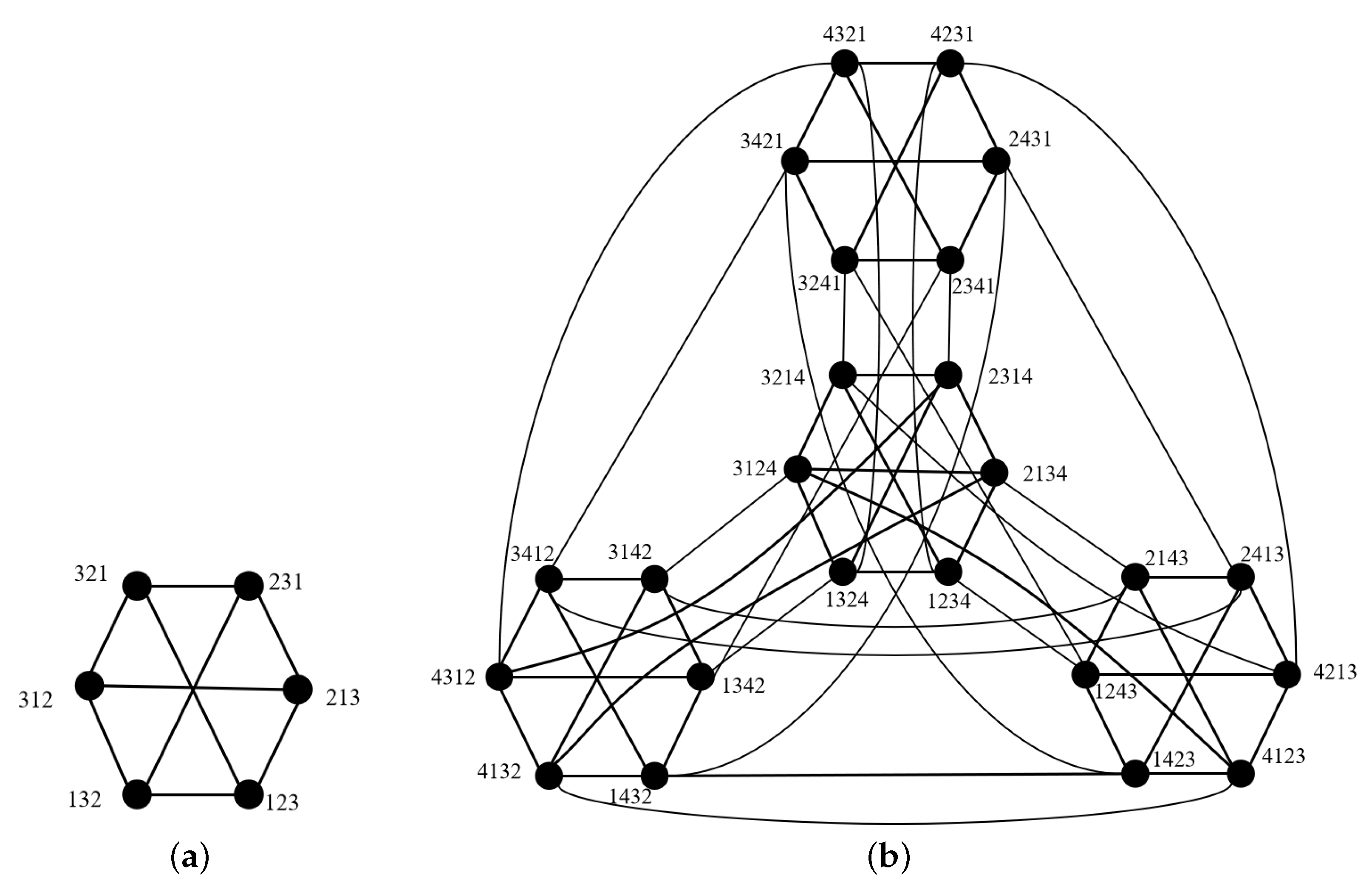
The graphs $B{S}_3$ and $B{S}_4$ are depicted in Figure 1. We can see from the definition that $B{S}_n$ is a $(2n-3)$-regular bipartite graph. For any vertex $\mu$ in $B{S}_n$, $N\left(\mu \right)=\left\{{\mu }_1^j\right|2\le j\le n\}\bigcup \left\{{\mu }_j^{j+1}\right|2\le j\le n-1\}$. In addition, $B{S}_n$ is a Cayley graph with vertex symmetry. $B{S}_n$ is composed of n subgraphs $B{S}_n^1$, $B{S}_n^2$, …, $B{S}_n^n$, where each $B{S}_n^i(1\le i\le n)$ is isomorphic to $B{S}_{n-1}$.

3. Structure Fault Tolerance of ${\mathit{BS}}_{\mathit{n}}$

We first prove $\kappa (B{S}_n;H)$ and ${\kappa }^s(B{S}_n;H)$ for any integer $n\ge 4$, where $H\in \{K_1,K_{1,1},K_{1,2}\}$. Then, we study the upper bounds for $\kappa (B{S}_n;K_{1,3})$ and ${\kappa }^s(B{S}_n;K_{1,3})$.

Lemma 1

(see [19]) For $n\ge 3$, $\kappa \left(B{S}_n\right)=\lambda \left(B{S}_n\right)=2n-3$.

By Lemma 1, we can easily get the results as follows.

Theorem 1.

$\kappa (B{S}_n;K_1)=2n-3$ and ${\kappa }^s(B{S}_n;K_1)=2n-3$ for any integer $n\ge 4$.

Lemma 2

(see [19]). For $n\ge 2$, $\kappa \lambda \left(B{S}_n\right)=2n-3$.

Lemma 3.

Let μ be any vertex in $B{S}_n$ and let $\nu ={\mu }_2^3$ for $n\ge 4$. Then, $({\mu }_1^i,{\nu }_1^i)\in E\left(B{S}_n\right)$ for $2\le i\le n$ and $({\mu }_i^{i+1},{\nu }_i^{i+1})\in E\left(B{S}_n\right)$ for $4\le i\le n-1$.

Proof.

Let $\mu ={\mu }_1{\mu }_2{\mu }_3\dots {\mu }_i{\mu }_{i+1}\dots {\mu }_n$. Then, $\nu ={\mu }_1{\mu }_3{\mu }_2\dots {\mu }_i{\mu }_{i+1}\dots {\mu }_n$. We have ${\mu }_1^i={\mu }_i{\mu }_2{\mu }_3\dots {\mu }_1{\mu }_{i+1}\dots {\mu }_n$ and ${\nu }_1^i={\mu }_i{\mu }_3{\mu }_2\dots {\mu }_1{\mu }_{i+1}\dots {\mu }_n$ for $4\le i\le n$. Since ${\left({\mu }_1^i\right)}_2^3={\nu }_1^i$, then $({\mu }_1^i,{\nu }_1^i)\in E\left(B{S}_n\right)$ for $4\le i\le n$. Again, we have ${\mu }_1^2={\mu }_2{\mu }_1{\mu }_3\dots {\mu }_i{\mu }_{i+1}\dots {\mu }_n$, ${\mu }_1^3={\mu }_3{\mu }_2{\mu }_1\dots {\mu }_i{\mu }_{i+1}\dots {\mu }_n$, ${\nu }_1^2={\mu }_3{\mu }_1{\mu }_2\dots {\mu }_i{\mu }_{i+1}\dots {\mu }_n$, and ${\nu }_1^3={\mu }_2{\mu }_3{\mu }_1\dots {\mu }_i{\mu }_{i+1}\dots {\mu }_n$. Then, ${\left({\mu }_1^2\right)}_1^3={\nu }_1^2$ and ${\left({\mu }_1^3\right)}_1^2={\nu }_1^3$. Hence, $({\mu }_1^i,{\nu }_1^i)\in E\left(B{S}_n\right)$ for $2\le i\le n$. Similarly, ${\mu }_i^{i+1}={\mu }_1{\mu }_2{\mu }_3\dots {\mu }_{i+1}{\mu }_i\dots {\mu }_n$ and ${\nu }_i^{i+1}={\mu }_1{\mu }_3{\mu }_2\dots {\mu }_{i+1}{\mu }_i\dots {\mu }_n$ for $4\le i\le n-1$. Since ${\left({\mu }_i^{i+1}\right)}_2^3={\nu }_i^{i+1}$, then $({\mu }_i^{i+1},{\nu }_i^{i+1})\in E\left(B{S}_n\right)$ for $4\le i\le n-1$. □

Lemma 4.

For $n\ge 4$, $\kappa (B{S}_n;K_{1,1})\le 2n-3$ and ${\kappa }^s(B{S}_n;K_{1,1})\le 2n-3$.

Proof.

Let $\mu =12\dots n$ and $\nu ={\mu }_2^3$. We set $H=\left\{\{{\mu }_1^i,{\nu }_1^i\}\right|2\le i\le n\}\cup \left\{\{{\mu }_i^{i+1},{\nu }_i^{i+1}\}\right|4\le i\le n-1\}\cup \{\{{\mu }_3^4,{\left({\mu }_3^4\right)}_1^2\},\{{\nu }_3^4,{\left({\nu }_3^4\right)}_1^2\}\}$. Then, $\left|H\right|=n-1+n-4+2=2n-3$. Obviously, $N\left(\right\{\mu ,\nu \left\}\right)\subset V\left(H\right)$. Then, $B{S}_n-V\left(H\right)$ is disconnected and $\{\mu ,\nu \}$ is a component of $B{S}_n-V\left(H\right)$. By Lemma 3, each $H_i\in H$ is isomorphic to $K_{1,1}$, and we get $\kappa (B{S}_n;K_{1,1})\le 2n-3$ and ${\kappa }^s(B{S}_n;K_{1,1})\le 2n-3$. See Figure 2 for an illustration. □

Lemma 5.

For $n\ge 4$, ${\kappa }^s(B{S}_n;K_{1,1})\ge 2n-3$ and $\kappa (B{S}_n;K_{1,1})\ge 2n-3$.

Proof.

Let $H=\left\{T_i\right|1\le i\le 2n-4\}$ be a subgraph set of $B{S}_n$, where each $T_i$ is isomorphic to a connected subgraph of $K_{1,1}$. To prove ${\kappa }^s(B{S}_n;K_{1,1})\ge 2n-3$, we need to show that $B{S}_n-V\left(H\right)$ is connected. Let $H_e=H\cap E\left(B{S}_n\right)$ and $H_v=H-H_e$. We consider the following three cases.

Case 1. $|H_v|=|H|$.

In this case, $\left|V\right(H\left)\right|\le 2n-4$. Since $\kappa \left(B{S}_n\right)=2n-3$, $B{S}_n-V\left(H\right)$ is connected.

Case 2. $|H_e|=|H|$.

In this case, $\left|E\right(H\left)\right|\le 2n-4$. Since $\lambda \left(B{S}_n\right)=2n-3$, $B{S}_n-V\left(H\right)$ is connected.

Case 3. $0<|H_v|<|H|$ and $0<|H_e|<|H|$.

In this case, $|H_e|+|H_v|=|H|\le 2n-4$. By Lemma 2, $B{S}_n-V\left(H\right)$ is connected.

Hence, ${\kappa }^s(B{S}_n;K_{1,1})\ge 2n-3$ and $\kappa (B{S}_n;K_{1,1})\ge 2n-3$. □

According to Lemmas 4 and 5, we have Theorem 2.

Theorem 2.

$\kappa (B{S}_n;K_{1,1})=2n-3$ and ${\kappa }^s(B{S}_n;K_{1,1})=2n-3$ for any integer $n\ge 4$.

Lemma 6.

For $n\ge 4$, $\kappa (B{S}_n;K_{1,2})\le n-1$ and ${\kappa }^s(B{S}_n;K_{1,2})\le n-1$.

Proof.

Let $\mu =12\dots n$ and $H=\left\{\{{\mu }_1^i,{\left({\mu }_1^i\right)}_1^{i+1},{\mu }_i^{i+1}\}\right|2\le i\le n-1\}\cup \{{\mu }_1^n,{\left({\mu }_1^n\right)}_1^2,{\left({\mu }_1^n\right)}_2^3\}$. Then, $\left|H\right|=n-2+1=n-1$. Since $N\left(\mu \right)\subset V\left(H\right)$, $B{S}_n-V\left(H\right)$ is disconnected, and one component of $B{S}_n-V\left(H\right)$ is $\left\{\mu \right\}$. Since $({\mu }_1^i,{\left({\mu }_1^i\right)}_1^{i+1}),({\left({\mu }_1^i\right)}_1^{i+1},{\mu }_i^{i+1})\in E\left(B{S}_n\right)$, each element in H is isomorphic to $K_{1,2}$, where ${\left({\mu }_1^i\right)}_1^{i+1}$ is the center vertex. Then, we get $\kappa (B{S}_n;K_{1,2})\le n-1$ and ${\kappa }^s(B{S}_n;K_{1,2})\le n-1$. See Figure 3 for an illustration. □

Lemma 7.

Let μ be any vertex in $B{S}_n$, let $M\cong K_{1,2}$ be any connected subgraph in $B{S}_n$, and let $c(M\cap N(\mu \left)\right)$ be the maximum number of neighbors of μ that can be contained in M. Then, $c(M\cap N(\mu \left)\right)\le 2$.

Proof.

Let $V\left(M\right)=\left\{{\mu }_i\right|0\le i\le 2\}$, where ${\mu }_1$ is the center vertex of M. Suppose that $c(M\cap N(\mu \left)\right)$=3. Then, we have two $C_3$: $\{{\mu }_0,{\mu }_1,\mu \}$ and $\{{\mu }_2,{\mu }_1,\mu \}$. Since $B{S}_n$ is bipartite, there is no $C_3$ in $B{S}_n$, and we get a contradiction. Hence, $c(M\cap N(\mu \left)\right)\le 2$. □

Lemma 8.

Let $H=\{H_1,H_2,\dots ,H_t\}$ be a subgraph set of $B{S}_n$, where each $H_i\in H$ is isomorphic to a connected subgraph of $K_{1,2}$. If $t\le n-2$, then $B{S}_n-V\left(H\right)$ is connected.

Proof.

Suppose that $\mu$ is any vertex in $B{S}_n$. Let $s=\sum _{i=1}^{t}c(H_i,N\left(\mu \right))$. By Lemma 7, $s\le 2(n-2)=2n-4<2n-3=\kappa \left(B{S}_n\right)$. Then, by Lemma 1, $B{S}_n-V\left(H\right)$ is connected. □

According to Lemma 8, we have Lemma 9.

Lemma 9.

For $n\ge 4$, $\kappa (B{S}_n;K_{1,2})\ge n-1$ and ${\kappa }^s(B{S}_n;K_{1,2})\ge n-1$.

According to Lemmas 6 and 9, we have Theorem 3.

Theorem 3.

$\kappa (B{S}_n;K_{1,2})=n-1$ and ${\kappa }^s(B{S}_n;K_{1,2})=n-1$ for any integer $n\ge 4$.

Lemma 10.

Let μ be any vertex in $B{S}_n$, and let ${\mu }_1^i$, ${\mu }_1^{i+1}$ and ${\mu }_i^{i+1}$ have a common neighbor in $B{S}_n$ for $2\le i\le n-1$ and $n\ge 4$.

Proof.

Let $\mu =x_1\dots x_i{x}_{i+1}\dots x_n$. Then, ${\mu }_1^i=x_i\dots x_1{x}_{i+1}\dots x_n$, ${\mu }_1^{i+1}=x_{i+1}\dots x_i{x}_1\dots x_n$, and ${\mu }_i^{i+1}=x_1\dots x_{i+1}{x}_i\dots x_n$. Let $\nu ={\left({\mu }_1^i\right)}_1^{i+1}=x_{i+1}\dots x_1{x}_i\dots x_n$. Then, $({\mu }_1^i,\nu )\in E\left(B{S}_n\right)$. Since ${\left({\mu }_1^{i+1}\right)}_i^{i+1}=x_{i+1}\dots x_1{x}_i\dots x_n=\mu$ and ${\left({\mu }_i^{i+1}\right)}_1^i=x_{i+1}\dots x_1{x}_i\dots x_n=\mu$, $({\mu }_1^{i+1},\nu ),({\mu }_i^{i+1},\nu )\in E\left(B{S}_n\right)$. Hence, $\nu$ is the common neighbor of ${\mu }_1^i$,${\mu }_1^{i+1}$ and ${\mu }_i^{i+1}$. □

Lemma 11.

Let μ be any vertex in $B{S}_n$, and let ${\mu }_i^{i+1}$ and ${\mu }_{i+2}^{i+3}$ have a common neighbor in $B{S}_n$ for i with $2\le i\le n-3$ and $n\ge 4$.

Proof.

Let $\mu =x_1\dots x_i{x}_{i+1}{x}_{i+2}{x}_{i+3}\dots x_n$. Then, ${\mu }_i^{i+1}=x_1\dots x_{i+1}{x}_i{x}_{i+2}{x}_{i+3}\dots x_n$, ${\mu }_{i+2}^{i+3}=x_1\dots x_i{x}_{i+1}{x}_{i+3}{x}_{i+2}\dots x_n$. Let $\nu ={\left({\mu }_i^{i+1}\right)}_{i+2}^{i+3}=x_1\dots x_{i+1}{x}_i{x}_{i+3}{x}_{i+2}\dots x_n$. Then, $({\mu }_i^{i+1},\nu )\in E\left(B{S}_n\right)$. Since ${\left({\mu }_{i+2}^{i+3}\right)}_i^{i+1}=x_1\dots x_{i+1}{x}_i{x}_{i+3}{x}_{i+2}\dots x_n=\nu$, then $({\mu }_{i+2}^{i+3},\nu )\in E\left(B{S}_n\right)$. Hence, $\nu$ is the common neighbor of ${\mu }_i^{i+1}$ and ${\mu }_{i+2}^{i+3}$. □

Lemma 12.

For $n\ge 4$,

$${\kappa }^s(B{S}_n;K_{1,3})\le \kappa (B{S}_n;K_{1,3})\le \left\{\begin{array}{cc}\frac{3(n-1)}{4}\hfill & \mathit{if}(n-1)\%4=0\hfill \\ \frac{3(n-2)}{4}+1\hfill & \mathit{if}(n-2)\%4=0\hfill \\ \frac{3(n-3)}{4}+1\hfill & \mathit{if}(n-3)\%4=0\hfill \\ \frac{3(n-4)}{4}+2\hfill & \mathit{if}(n-4)\%4=0.\hfill \end{array}\right.$$

Proof.

Let $\mu$ be any vertex in $B{S}_n$. Each $\mu$ has n neighbors $N\left(\mu \right)=\left\{{\mu }_1^i\right|2\le i\le n\}\bigcup \left\{{\mu }_i^{i+1}\right|2\le i\le n-1\}$, so we can construct $K_{1,3}$ with $N\left(\mu \right)$. According to Lemma 10, we can construct $H_1=\left\{\{{\mu }_1^{2i},{\mu }_1^{2i+1},{\mu }_{2i}^{2i+1},{\left({\mu }_1^{2i}\right)}_1^{2i+1}\}\right|1\le i\le \frac{n-1}{2}\}$, which has $\frac{n-1}{2}$$K_{1,3}$ when n is odd. In addition, we can construct $H_1=\left\{\{{\mu }_1^{2i},{\mu }_1^{2i+1},{\mu }_{2i}^{2i+1},{\left({\mu }_1^{2i}\right)}_1^{2i+1}\}\right|1\le i\le \frac{n-2}{2}\}$, which has $\frac{n-2}{2}$$K_{1,3}$ when n is even. By Lemma 11, we can construct $K_{1,3}$ with ${\mu }_{4i-1}^{4i}$ and ${\mu }_{4i+1}^{4i+2}$ for $i\ge 1$. Then, if there are still vertices left, we can build $K_{1,3}$ with these vertices and their neighbors. We have the following four cases.

Case 1. $(n-1)\%4=0$.

We can construct $K_{1,3}$ as follows:

$H_1=\left\{\{{\mu }_1^{2i},{\mu }_1^{2i+1},{\mu }_{2i}^{2i+1},{\left({\mu }_1^{2i}\right)}_1^{2i+1}\}\right|1\le i\le \frac{n-1}{2}\},$

$H_2=\left\{\{{\mu }_{4i-1}^{4i},{\mu }_{4i+1}^{4i+2},{\left({\mu }_{4i-1}^{4i}\right)}_{4i+1}^{4i+2},{\left({\left({\mu }_{4i-1}^{4i}\right)}_{4i+1}^{4i+2}\right)}_1^2\}\right|1\le i\le \frac{n-5}{4}\}$,

$H_3=\left\{\{{\mu }_{n-2}^{n-1},{\left({\mu }_{n-2}^{n-1}\right)}_1^2,{\left({\mu }_{n-2}^{n-1}\right)}_1^3,{\left({\mu }_{n-2}^{n-1}\right)}_1^4\}\right\}$.

Let $H=H_1\cup H_2\cup H_3$. Then, $\left|H\right|=\frac{n-1}{2}+\frac{n-5}{4}+1=\frac{3(n-1)}{4}$. Since $N\left(\mu \right)\subset V\left(H\right)$, $B{S}_n-V\left(H\right)$ is disconnected and $\mu$ is a component of $B{S}_n-V\left(H\right)$. For each $H_i$ in H is isomorphic to $K_{1,3}$, we have $\kappa (B{S}_n;K_{1,3})\le \frac{3(n-1)}{4}$ and ${\kappa }^s(B{S}_n;K_{1,3})\le \frac{3(n-1)}{4}$.

Case 2. $(n-2)\%4=0$.

We can construct $K_{1,3}$ as follows:

$H_1=\left\{\{{\mu }_1^{2i},{\mu }_1^{2i+1},{\mu }_{2i}^{2i+1},{\left({\mu }_1^{2i}\right)}_1^{2i+1}\}\right|1\le i\le \frac{n-2}{2}\},$

$H_2=\left\{\{{\mu }_{4i-1}^{4i},{\mu }_{4i+1}^{4i+2},{\left({\mu }_{4i-1}^{4i}\right)}_{4i+1}^{4i+2},{\left({\left({\mu }_{4i-1}^{4i}\right)}_{4i+1}^{4i+2}\right)}_1^2\}\right|1\le i\le \frac{n-2}{4}\}$,

$H_3=\left\{\{{\mu }_1^n,{\left({\mu }_1^n\right)}_1^2,{\left({\mu }_1^n\right)}_1^3,{\left({\mu }_1^n\right)}_1^4\}\right\}$.

Let $H=H_1\cup H_2\cup H_3$. Then, $\left|H\right|=\frac{n-2}{2}+\frac{n-2}{4}+1=\frac{3(n-2)}{4}+1$. Since $N\left(\mu \right)\subset V\left(H\right)$, $B{S}_n-V\left(H\right)$ is disconnected and $\mu$ is a component of $B{S}_n-V\left(H\right)$. For each $H_i$ in H is isomorphic to $K_{1,3}$, we have $\kappa (B{S}_n;K_{1,3})\le \frac{3(n-2)}{4}+1$ and ${\kappa }^s(B{S}_n;K_{1,3})\le \frac{3(n-2)}{4}+1$.

Case 3. $(n-3)\%4=0$.

We can construct $K_{1,3}$ as follows:

$H_1=\left\{\{{\mu }_1^{2i},{\mu }_1^{2i+1},{\mu }_{2i}^{2i+1},{\left({\mu }_1^{2i}\right)}_1^{2i+1}\}\right|1\le i\le \frac{n-1}{2}\},$

$H_2=\left\{\{{\mu }_{4i-1}^{4i},{\mu }_{4i+1}^{4i+2},{\left({\mu }_{4i-1}^{4i}\right)}_{4i+1}^{4i+2},{\left({\left({\mu }_{4i-1}^{4i}\right)}_{4i+1}^{4i+2}\right)}_1^2\}\right|1\le i\le \frac{n-3}{4}\}$,

Let $H=H_1\cup H_2$. Then, $\left|H\right|=\frac{n-1}{2}+\frac{n-3}{4}=\frac{3(n-3)}{4}+1$. Since $N\left(\mu \right)\subset V\left(H\right)$, $B{S}_n-V\left(H\right)$ is disconnected and $\mu$ is a component of $B{S}_n-V\left(H\right)$. For each $H_i$ in H is isomorphic to $K_{1,3}$, we have $\kappa (B{S}_n;K_{1,3})\le \frac{3(n-3)}{4}+1$ and ${\kappa }^s(B{S}_n;K_{1,3})\le \frac{3(n-3)}{4}+1$.

Case 4. $(n-4)\%4=0$.

We can construct $K_{1,3}$ as follows:

$H_1=\left\{\{{\mu }_1^{2i},{\mu }_1^{2i+1},{\mu }_{2i}^{2i+1},{\left({\mu }_1^{2i}\right)}_1^{2i+1}\}\right|1\le i\le \frac{n-2}{2}\},$

$H_2=\left\{\{{\mu }_{4i-1}^{4i},{\mu }_{4i+1}^{4i+2},{\left({\mu }_{4i-1}^{4i}\right)}_{4i+1}^{4i+2},{\left({\left({\mu }_{4i-1}^{4i}\right)}_{4i+1}^{4i+2}\right)}_1^2\}\right|1\le i\le \frac{n-4}{4}\}$,

$H_3=\left\{\{{\mu }_1^n,{\mu }_{n-1}^n,{\left({\mu }_{n-1}^n\right)}_1^n,{\left({\left({\mu }_{n-1}^n\right)}_1^n\right)}_1^2\}\right\}$.

Let $H=H_1\cup H_2\cup H_3$. Then, $\left|H\right|=\frac{n-2}{2}+\frac{n-4}{4}+1=\frac{3(n-4)}{4}+2$. Since $N\left(\mu \right)\subset V\left(H\right)$, $B{S}_n-V\left(H\right)$ is disconnected and $\mu$ is a component of $B{S}_n-V\left(H\right)$. For each $H_i$ in H is isomorphic to $K_{1,3}$, we have $\kappa (B{S}_n;K_{1,3})\le \frac{3(n-4)}{4}+2$ and ${\kappa }^s(B{S}_n;K_{1,3})\le \frac{3(n-4)}{4}+2$. See Figure 4 for an illustration. □

According to the proof, we give an algorithm for calculating the upper bounds of the $K_{1,3}$-(sub)structure connectivity of $B{S}_n$ (see Algorithm 1). We performed a simulation based on this algorithm to get the upper bounds of the $K_{1,3}$-(sub)structure connectivity when the dimension was $n\le 9$. The results obtained from the algorithm are consistent with those of Lemma 12, please see

Table 1. The upper bounds of $K_{1,3}$-(sub)structure connectivity.

	n = 4	n = 5	n = 6	n = 7	n = 8	n = 9
κ(BSn,K1,3) ≤	2	3	4	4	5	5
κS(BSn,K1,3) ≤	2	3	4	4	5	6

for reference.

Algorithm 1 Calculate the upper bounds of $K_{1,3}$-(sub)structure connectivity

Input: node $\mu$, dimension n

Output: upper bounds of $K_{1,3}$-(sub)structure connectivity

1 switch n%4 do

2 case 0:

3       for $i\leftarrow 1$to$\frac{n-2}{2}$ do

4             construct $K_{1,3}$ with {${\mu }_1^{2i},{\mu }_1^{2i+1},{\mu }_{2i}^{2i+1},{\left({\mu }_1^{2i}\right)}_1^{2i+1}$};

5       for $i\leftarrow 1$to$\frac{n-4}{4}$ do

6             construct $K_{1,3}$ with {${\mu }_{4i-1}^{4i},{\mu }_{4i+1}^{4i+2},{\left({\mu }_{4i-1}^{4i}\right)}_{4i+1}^{4i+2},{\left({\left({\mu }_{4i-1}^{4i}\right)}_{4i+1}^{4i+2}\right)}_1^2$};

7       construct $K_{1,3}$ with {${\mu }_1^n,{\mu }_{n-1}^n,{\left({\mu }_{n-1}^n\right)}_1^n,{\left({\left({\mu }_{n-1}^n\right)}_1^n\right)}_1^2\}$}

8 case 1:

9       for $i\leftarrow 1$to$\frac{n-1}{2}$ do

10             construct $K_{1,3}$ with {${\mu }_1^{2i},{\mu }_1^{2i+1},{\mu }_{2i}^{2i+1},{\left({\mu }_1^{2i}\right)}_1^{2i+1}$};

11       for $i\leftarrow 1$to$\frac{n-5}{4}$ do

12             construct $K_{1,3}$ with {${\mu }_{4i-1}^{4i},{\mu }_{4i+1}^{4i+2},{\left({\mu }_{4i-1}^{4i}\right)}_{4i+1}^{4i+2},{\left({\left({\mu }_{4i-1}^{4i}\right)}_{4i+1}^{4i+2}\right)}_1^2$};

13       construct $K_{1,3}$ with {${\mu }_{n-2}^{n-1},{\left({\mu }_{n-2}^{n-1}\right)}_1^2,{\left({\mu }_{n-2}^{n-1}\right)}_1^3,{\left({\mu }_{n-2}^{n-1}\right)}_1^4$};

14 case 2:

15       for $i\leftarrow 1$to$\frac{n-2}{2}$ do

16             construct $K_{1,3}$ with {${\mu }_1^{2i},{\mu }_1^{2i+1},{\mu }_{2i}^{2i+1},{\left({\mu }_1^{2i}\right)}_1^{2i+1}$};

17       for $i\leftarrow 1$to$\frac{n-2}{4}$ do

18             construct $K_{1,3}$ with {${\mu }_{4i-1}^{4i},{\mu }_{4i+1}^{4i+2},{\left({\mu }_{4i-1}^{4i}\right)}_{4i+1}^{4i+2},{\left({\left({\mu }_{4i-1}^{4i}\right)}_{4i+1}^{4i+2}\right)}_1^2$};

19       construct $K_{1,3}$ with {${\mu }_1^n,{\left({\mu }_1^n\right)}_1^2,{\left({\mu }_1^n\right)}_1^3,{\left({\mu }_1^n\right)}_1^4$};

20 case 3:

21       for $i\leftarrow 1$to$\frac{n-1}{2}$ do

22             construct $K_{1,3}$ with {${\mu }_1^{2i},{\mu }_1^{2i+1},{\mu }_{2i}^{2i+1},{\left({\mu }_1^{2i}\right)}_1^{2i+1}$};

23       for $i\leftarrow 1$to$\frac{n-3}{4}$ do

24             construct $K_{1,3}$ with {${\mu }_{4i-1}^{4i},{\mu }_{4i+1}^{4i+2},{\left({\mu }_{4i-1}^{4i}\right)}_{4i+1}^{4i+2},{\left({\left({\mu }_{4i-1}^{4i}\right)}_{4i+1}^{4i+2}\right)}_1^2$};

25 end

4. Conclusions

The connectivity of a network is a significant indicator for measuring that network’s fault tolerance properties. In order to assess the impact of structure failure, structure connectivity and substructure connectivity are presented. In this paper, we find the upper bounds of $\kappa (B{S}_n;K_{1,3})$ and ${\kappa }^s(B{S}_n;K_{1,3})$. Furthermore, we establish $\kappa (B{S}_n;H)$ and ${\kappa }^s(B{S}_n;H)$ of $B{S}_n$, where $H\in \{K_1,K_{1,1},K_{1,2}\}$.

A hypercube $Q_n$ is an efficient symmetric network that has been used for commercial high-performance computers. The star graph $S_n$ and bubble-sort graph $B_n$ are two alternatives to the hypercube. $B{S}_n$, which is generated by merging $B_n$ and $S_n$, has the advantages of both $B_n$ and $S_n$. Here, we compare the H-(sub)structure connectivity of $Q_n$, $B_n$, $S_n$, and $B{S}_n$ for $H\in \{K_1,K_{1,1},K_{1,2}\}$. As shown in Table

Table 2. This is a table.

	Dimension	K1	K1,1	K1,2
Qn	7	7	6	4
Sn	7	6	6	6
Bn	7	6	6	3
BSn	7	11	11	6
Qn	8	8	7	4
Sn	8	7	7	7
Bn	8	7	7	4
BSn	8	13	13	7
Qn	9	9	8	5
Sn	9	8	8	8
Bn	9	8	8	4
BSn	9	15	15	8
Qn	10	10	9	5
Sn	10	9	9	9
Bn	10	9	9	5
BSn	10	17	17	9

, $B{S}_n$ has the highest $K_1$-(sub)structure connectivity and $K_{1,1}$-(sub)structure connectivity among these four networks. In addition, $B{S}_n$ has the same $K_{1,2}$-(sub)structure connectivity as that of $S_n$, which is larger than those of $Q_n$ and $B_n$. The comparison shows that $B{S}_n$ is more stable than $Q_n$, $S_n$, and $B_n$, when structure faults occur.

References

- West, D.B. Introduction to Graph Theory; Prentice Hall Publishers: Englewood Cliffs, NJ, USA, 2001. [Google Scholar]
- Harary, F. Conditional connectivity. Networks 1983, 13, C347–C357. [Google Scholar] [CrossRef]
- Fabrega, J.; Fiol, M.A. On the extraconnectivity of graphs. Discret. Math. 1996, 155, C49–C57. [Google Scholar] [CrossRef]
- Esfahanian, A.H.; Hakimi, S.L. On computing a conditional edge-connectivity of a graph. Inform. Process. Lett. 1988, 27, 195–199. [Google Scholar] [CrossRef]
- Esfahanian, A.H. Generalized measures of fault tolerance with application to n-cube networks. IEEE Trans. Comput. 1989, 38, 1586–1591. [Google Scholar] [CrossRef]
- Latifi, S.; Hegde, M.; Pour, M.N. Conditional connectivity measures for large multiprocessor systems. IEEE Trans. Comput. 1994, 43, 218–222. [Google Scholar] [CrossRef]
- Lin, C.-K.; Zhang, L.; Fan, J.; Wang, D. Structure connectivity and substructure connectivity of hypercubes. Theor. Comput. Sci. 2016, 634, 97–107. [Google Scholar] [CrossRef]
- Lv, Y.; Fan, J.; Hsu, D.F.; Lin, C.-K. Structure connectivity and substructure connectivity of k-ary n-cube networks. Inf. Sci. 2018, 433–434, 115–124. [Google Scholar] [CrossRef]
- Lv, H.; Wu, T. Structure and substructure connectivity of balanced hypercubes. Bull. Malaysian Math. Sci. Soc. 2020, 43, 2659–2672. [Google Scholar]
- Li, D.; Hu, X.; Liu, H. Structure connectivity and substructure connectivity of twisted hypercubes. Theor. Comput. Sci. 2019, 796, 169–179. [Google Scholar] [CrossRef]
- Sabir, E.; Meng, J. Structure fault tolerance of hypercubes and folded hypercubes. Theor. Comput. Sci. 2018, 711, C44–C55. [Google Scholar] [CrossRef]
- You, L.; Han, Y.; Wang, X.; Zhou, C.; Gu, R.; Lu, C. Structure connectivity and substructure connectivity of alternating group graphs. In Proceedings of the 2018 IEEE International Conference on Progress in Informatics and Computing (PIC), Suzhou, China, 14–16 December 2018; pp. 317–321. [Google Scholar]
- Li, X.; Zhou, S.; Ren, X.; Guo, X. Structure and substructure connectivity of alternating group graphs. Appl. Math. Comput. 2021, 391, 125639. [Google Scholar] [CrossRef]
- Zhang, G.; Wang, D. Structure connectivity and substructure connectivity of bubble-sort star graph networks. Appl. Math. Comput. 2019, 363, 124632. [Google Scholar] [CrossRef]
- Zhang, G.; Lin, S. Path and cycle fault tolerance of bubble-sort graph networks. Theor. Comput. Sci. 2019, 779, 8–16. [Google Scholar] [CrossRef]
- Feng, W.; Wang, S. Structure connectivity and substructure connectivity of wheel networks. Theor. Comput. Sci. 2021, 850, 20–29. [Google Scholar] [CrossRef]
- Akers, S.B.; Krishnamurthy, B. A group-theoretic model for symmetric interconnection networks. IEEE Trans. Comput. 1989, 38, 555–566. [Google Scholar] [CrossRef]
- Chou, Z.; Hsu, C.; Sheu, J. Bubble-sort star graphs: A new interconnection network. In Proceedings of the International Conference on Parallel and Distributed Systems, Tokyo, Japan, 3–6 June 1996; pp. 41–48. [Google Scholar]
- Wang, S.; Wang, M. The strong connectivity of bubble-sort star graphs. Comput. J. 2018, 62, 715–729. [Google Scholar] [CrossRef]
Figure 1.
The graphs (a) and (b) .
Figure 2.
An example of and , where .
Figure 3.
An example of and where .