Abstract
In the face of increasing flood risks intensified by climate change, accurate flood inundation mapping is pivotal for effective disaster management. This study introduces a novel explainable deep learning architecture designed to generate precise flood inundation maps from diverse satellite data sources. A comprehensive evaluation of the proposed model is conducted, comparing it with state-of-the-art models across various fusion configurations of Multispectral Optical and Synthetic Aperture Radar (SAR) images. The proposed model consistently outperforms other models across both Sentinel-1 and Sentinel-2 images, achieving an Intersection Over Union (IOU) of 0.5862 and 0.7031, respectively. Furthermore, analysis of the different fusion combinations reveals that the use of Sentinel-1 in combination with RGB, NIR, and SWIR achieves the highest IOU of 0.7053 and that the inclusion of the SWIR band has the greatest positive impact on the results. Gradient-weighted class activation mapping is employed to provide insights into its decision-making processes, enhancing transparency and interpretability. This research contributes significantly to the field of flood inundation mapping, offering an efficient model suitable for diverse applications. This study not only advances flood inundation mapping but also provides a valuable tool for improved understanding of deep learning decision-making in this area, ultimately contributing to improved disaster management strategies.
1. Introduction
Climate change is increasingly manifesting in the forms of higher temperatures and more intense storms, leading to a rise in both the frequency and severity of flooding [1]. These climate-induced events underline the imperative need to develop effective flood-resilience measures, with a focus on early detection for managing and mitigating associated risks [2]. Flood management holds a critical role in achieving Sustainable Development Goals (SDGs) related to clean water and sanitation (SDG 6); sustainable cities and communities (SDG 11); and climate action (SDG 13).
Recent data from the Centre for Research on the Epidemiology of Disasters revealed that floods accounted for over 47% of weather-related disasters between 1995 and 2015. This alarming statistic underscores the urgency of transitioning to a resilience-based approach to flood risk management [3]. This approach, in line with SDG 6, recognizes that floods can have a direct impact on water quality and sanitation by causing contamination and damaging infrastructure. Effectively managing floods becomes integral to achieving the goal of clean water and sanitation, ensuring that flooding does not jeopardize the well-being and health of affected communities.
In recent years, uncontrolled urban expansion and unplanned development have encroached upon floodplains, obstructing natural water flows and escalating flood risks, leading to extensive financial losses. Accurate flood inundation mapping plays a crucial role in guiding urban planning to mitigate these challenges [4]. This aligns directly with SDG 11, emphasizing the need for sustainable and resilient human settlements. Planning developments in a way that prevents the encroachment of settlements onto flood-prone areas is essential for ensuring the safety, resilience, and sustainability of communities and urban environments, which are crucial for achieving SDG 11 and its focus on building resilient and inclusive cities.
A common approach to generating flood inundation maps is the pixel-level segmentation of satellite images. Two primary satellite sensors commonly used in generating flood inundation maps are synthetic aperture radar (SAR) and optical sensors. SAR sensors are capable of functioning regardless of the time of day and can penetrate cloud cover, making them ideal for regions prone to climate-induced cloud cover [5]. However, they come with the challenge of speckle noise, which can affect the accuracy of flood inundation mapping models. On the other hand, optical sensors provide a wealth of spectral information, allowing models to distinguish various features, such as vegetation and water. This can enhance the models’ ability to delineate floodwaters from other features when trained with optical imagery; however, they are unable to penetrate through cloud.
Alternatively, sub-pixel-level processing allows for the analysis of images with finer spatial detail, capturing information beyond the scale of individual pixels. This method involves estimating the fractional cover of specific features, such as water within a single pixel. Sub-pixel processing has proven to be a promising technique, particularly in developing more accurate flood inundation maps [6]. An associated approach, known as super-resolution mapping, further refines this concept. In super-resolution mapping, pixels are deconstructed into sub-pixels, and each sub-pixel is assigned a class label. This technique addresses the challenge of mixed pixels, common in low-resolution images where a single pixel may contain more than one type of land cover [7]. Although this has been shown to provide high levels of accuracy, it has a high computational cost, and can also be sensitive to noise, limiting its practical applicability.
The transition from traditional flood modeling techniques to advanced artificial intelligence, particularly machine and deep learning, is driven by the need for more accurate and efficient flood predictions [8]. These advances enable models to make quicker and more precise predictions. Deep learning, with its ability to learn complex relationships, is particularly suited for flood inundation mapping due to the complexity and widespread availability of satellite data. However, deep learning models are often considered “black boxes”, posing challenges regarding transparency and potential ethical biases, which can be addressed through the use of Explainable Artificial Intelligence (XAI). This study is focused on the application of XAI to flood inundation mapping, an area that is largely unexplored as far as the authors are aware, with only two existing works [9,10]. This approach offers enhanced insight into the behavior of the proposed deep learning model, as well as how this is impacted by varying input-data types [11].
1.1. Previous Work
1.1.1. Traditional Flood Inundation Mapping
Numerous techniques have been employed to map flood inundation from diverse satellite images. In the case of SAR images, the most common practice involves backscatter thresholding. Backscatter thresholding classifies a pixel as containing water if its backscatter value falls below a specified threshold [12]. In the context of optical imagery, flood inundation mapping involves techniques such as thresholding bands sensitive to water, like near-infrared (NIR) and shortwave-infrared (SWIR), or computing normalized difference indices like NDWI [13], MNDWI [14], and NDVI [15], where the normalized difference is found between NIR and SWIR; NIR and green; and NIR and red bands, respectively.
1.1.2. Artificial Intelligence for Flood Inundation Mapping
Recent advancements in machine learning and computer vision, coupled with increased computing power and extensive satellite data from programs like Copernicus, have spurred research into artificial intelligence’s application in flood inundation mapping. Although SAR images are commonly used due to their all-weather capability, some studies highlight the better performance of optical imagery. For instance, Bonafilia et al. [16] observed higher mean IOU values for Sentinel-2 compared to Sentinel-1. Similarly, Konapala et al. [17] reported higher F1 scores for Sentinel-2.
Traditional machine learning models have yielded accuracies ranging from 70% to 90%, but deep learning has demonstrated superior performance [18,19,20,21,22]. Deep learning models, particularly Convolutional Neural Networks (CNN), have been widely adopted for flood inundation mapping due to their ability to learn complex, non-linear relationships directly from raw data. They eliminate the need for extensive preprocessing, such as feature engineering. Models based on fully convolutional networks (FCN) have outperformed classical machine learning and traditional techniques [23].
To address resolution limitations introduced by convolutional layers, encoder–decoder architectures have been proposed. The U-Net model, a popular choice, features in several studies [5,17,24,25,26,27,28]. U-Net++ is a further state-of-the-art model that expands on U-Net, and it has been shown to achieve impressive performance in flood inundation mapping [29,30]; however, Helleis et al. [27] found that the standard U-Net performed better. Several studies have improved the performance of this architecture by incorporating attention mechanisms [31,32], demonstrably providing superior accuracy and efficiency.
Other architectures, like DeepLabV3 and DeepLabV3+, introduce innovative features such as atrous convolution, spatial pyramid pooling, and separable convolution, and they have been shown to outperform U-Net [27]. The choice of architecture and encoder module plays a critical role in model performance.
For SAR imagery, novel architectures have been introduced to improve performance. FWENet [33] combines aspects of U-Net and DeepLab, incorporating atrous convolution for enhanced results. Siam-DWENet [34], a Siamese network, learns differences between SAR images at various time intervals, outperforming other architectures. In optical imagery, H2O-Net [35] leverages generative adversarial networks to map RGB bands to SWIR signals, outperforming existing architectures trained with the original RGB bands.
One challenge in utilizing deep learning for flood inundation mapping is the need for large, labeled datasets, which can be time-consuming and costly to obtain. Efforts have been made to curate datasets like the Sen1Floods11 dataset. This paper aims to develop a deep learning semantic-segmentation model suitable for flood inundation mapping. The model’s appropriateness for this task as well as its performance are assessed by leveraging the Sen1Floods11 dataset.
The contributions of this paper are as follows:
- Presenting a novel deep learning semantic-segmentation model capable of producing high quality flood inundation maps from both SAR and optical images, demonstrated through comparative analysis with state-of-the-art models.
- Investigating various combinations of fusion of SAR and optical spectral bands and indices, providing insight into the optimal combinations for accurate flood inundation maps in both clear and cloud-covered conditions.
- Integrating XAI to interpret the behavior of the deep learning models, providing a more comprehensive understanding of their capacity to learn effectively. This not only enhances the trustworthiness of the models, but also provides deeper insight into the influence of each input-data type on the models’ decision-making process.
2. Materials and Methods
2.1. Dataset
The dataset employed in this research [16] comprises 446 images from Sentinel-1 and 446 images from Sentinel-2 satellites, both integral components of the European Space Agency’s Copernicus program, which is facilitating open access to satellite data. This dataset encompasses imagery from 11 distinct global flood events, occurring in Bolivia, Ghana, India, Cambodia, Nigeria, Pakistan, Paraguay, Somalia, Spain, Sri Lanka, and the USA, as depicted in Figure 1.
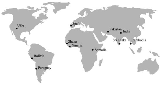
Figure 1.
Map showing the locations of the flood events sampled in the dataset.
Sentinel-1 satellites employ C-band SAR instruments, characterized by longer wavelengths compared to optical sensors. This feature enables them to penetrate through challenging conditions such as clouds, storms, and dense vegetation. Additionally, SAR sensors provide their own source of illumination, rendering them operational at any time of the day. Nonetheless, SAR imagery is susceptible to speckle, involving random signal variations, which can potentially impede the ability of deep learning models to discern authentic signals. The images selected for this study were captured in the interferometric wide swath (IW) mode, offering extensive coverage with an enhanced swath width of approximately 250 km. This mode is particularly well-suited for large-scale applications, including flood inundation mapping. The ground resolution in this imaging mode ranges between 5 and 20 m, and the images utilized in our study feature a ground resolution of 10 m. This moderate resolution strikes a balance between high- and low-level detail, ensuring visibility of smaller water bodies while adequately covering larger areas. The Sentinel-1 satellite offers various polarization modes, with the selected images featuring dual polarization, comprising vertical transmit and vertical-horizontal receive (VV + VH). This dual polarization mode enriches information for enhanced water detection while maintaining computational efficiency.
Conversely, Sentinel-2 satellites capture optical imagery using a multispectral instrument (MSI) with a 290 km field of view. This instrument records 13 spectral bands encompassing visible light, near-infrared, and shortwave-infrared spectra, offering detailed insights into vegetation, land cover, and water bodies. Such detailed information proves instrumental in distinguishing flooded areas from other land types. Among the 13 spectral bands, 4 feature a 10 m ground resolution, 6 have a 20 m ground resolution, and 3 exhibit a 60 m ground resolution. For the sake of consistency and improved analysis, the images were resampled to a uniform 10 m ground resolution for each band. A visual representation of the spectral bands from both satellites is illustrated in Figure 2.
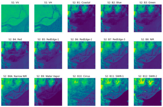
Figure 2.
Visualization of the two polarizations from a Sentinel-1 image, and the 13 spectral bands from a Sentinel-2 image taken from the flood event in India. Here the speckle in the Sentinel-1 images and the cloud coverage in the Sentinel-2 image can be clearly observed, highlighting the differences between the images from these two satellites.
The dataset comprises flood events for which both Sentinel-1 and coincident Sentinel-2 images were available within a maximum time frame of two days. Specifically, five events featured imagery captured on the same day, four within a one-day interval, and two with a two-day difference. Variations exist in the orbit direction, denoted as ascending (moving from the Southern to the Northern Hemisphere) or descending (moving from the Northern to the Southern Hemisphere), as well as in relative orbit values, signifying the satellite’s position and movement relative to other satellites in the constellation. An overview of this information for each event is provided in Table 1.

Table 1.
The dates, orbit direction and relative orbit value for each flood event.
2.1.1. Dataset Preparation
For the creation of ground truth labels, computation of NDVI and MNDWI values were performed using the Sentinel-2 images, followed by the application of predefined expert-defined thresholds: 0.2 for NDVI and 0.3 for MNDWI. These thresholds served to identify flooded and non-flooded pixels. Furthermore, analysts were granted access to the images and the initial labels obtained from Sentinel-2 data. They meticulously reviewed these labels and adjusted areas where water classifications required modification to non-water or vice versa. This meticulous review process enriched the quality of the labels, thus enhancing their utility in model training and evaluation.
To ensure the fidelity of the dataset, measures were implemented to remove cloud shadows that can exhibit a spectral signature similar to that of floodwater, potentially impeding the accurate classification of flooded pixels. This process involved identifying clouds by applying a threshold to the blue band, setting the threshold at 0.2, with values falling below this threshold being designated as indicative of clouds. Subsequently, the removal of cloud shadows was executed by projecting the cloud shadow based on factors such as potential cloud height, solar azimuth angle, and solar zenith angle.
2.1.2. Spectral Bands and Indices
The Sentinel-1 satellite is equipped with different polarization modes, encompassing both vertical and horizontal transmission and reception. Within this dataset, the satellite imagery features dual polarization, specifically vertical transmit and vertical/horizontal receive (VV + VH). This configuration provides enhanced information, contributing to the improved detection of water while simultaneously maintaining computational efficiency.
On the other hand, Sentinel-2 comprises a total of 13 spectral bands, offering a comprehensive range of information, as detailed in Table 2. Additionally, Figure 2 presents a visual representation of each spectral band for both Sentinel satellites.

Table 2.
Descriptions of each spectral band of Sentinel-2.
For flood inundation mapping, certain spectral bands are especially preferred. Notably, the visible light bands (RGB) are highly favored for their sensitivity to surface reflectance, rendering them effective in distinguishing various land-cover types, including water bodies. Furthermore, the near-infrared (NIR) band is frequently employed, as water bodies exhibit strong absorption of near-infrared light, facilitating a pronounced contrast between water and non-water regions. The shortwave-infrared (SWIR) bands are instrumental in capturing substantial information pertaining to surface moisture and are attuned to variations in water content.
The methodology for flood inundation mapping often relies on spectral indices, which are mathematical formulations combining pixel values from two or more spectral bands, designed to extract specific characteristics of the Earth’s surface based on reflectance values from diverse spectral bands, showing the relative abundance or lack of a specific land-cover type, for example, the Normalized Difference Water Index (NDWI), which extracts information about the presence of water bodies and the Normalized Difference Vegetation Index (NDVI), which extracts information about vegetation cover.
The NDWI is a fundamental index used in flood inundation mapping, due to its design for water detection, relying on the contrast in the reflectance between the green and NIR bands. The use of this index can be limited by noise emanating from built-up areas, vegetation, and soil, reducing the accuracy of resulting flood inundation maps. To address this challenge, the modified NDWI (MNDWI), shown in Equation (1), incorporates the SWIR band, which enhances the open water features, while diminishing the features of built-up areas, which are often correlated with open water when the NIR band is used. The NDVI, shown in Equation (2), finds utility in both vegetation detection and flood assessment, facilitated by its ability to distinguish between vegetation and water.
Considering the diverse strengths and limitations inherent to each satellite sensor, this study will assess the images from each satellite, alongside several distinct band-fusion configurations involving data from both satellites. The configurations that will be evaluated are as follows:
1. Sentinel-1 (VV + VH)
2. Sentinel-2 (All bands)
3. VV + VH + Sentinel-2 (All bands)
4. VV + VH + NIR
5. VV + VH + SWIR
6. VV + VH + NIR + SWIR
7. VV + VH + RGB
8. VV + VH + RGB + NIR
9. VV + VH + RGB + SWIR
10. VV + VH + RGB + NIR + SWIR
11. VV + VH + NDVI
12. VV + VH + MNDWI
2.2. Proposed Model Architecture
Encoder–decoder architectures are powerful methods of semantic segmentation. In this type of architecture, a fully convolutional CNN serves as the encoder module, responsible for extracting feature maps that capture high-level semantic information. A decoder module is employed to gradually up-sample the CNN’s output, thereby recovering the spatial information. The proposed model takes inspiration from this concept and incorporates two encoder and two decoder modules. The outputs from each are fused through a weighted average, utilizing two trainable weight parameters, W1 and W2, which are learned from the input data and optimized through the training process, where W1 is multiplied by the output of the powerful model and W2 is multiplied by the output of the lightweight model, and the resulting values are combined through element-wise addition. This combined output is subsequently processed through a fully connected layer and a sigmoid-activation function, leading to the final pixel-wise classification. This novel approach increases the input for the final classification task, thus enhancing performance, particularly given the constraints of a relatively small dataset. Furthermore, both encoder modules in our architecture are CNNs that have been pre-trained on ImageNet, then subsequently fine-tuned with the Sen1Floods11 dataset. A visual representation of this architecture is presented in Figure 3.
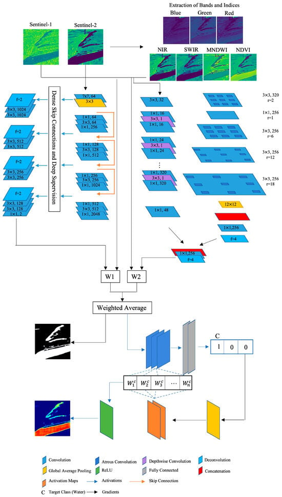
Figure 3.
Diagram of the proposed model architecture in which dual encoder-decoder models are adopted. The weights (W1 and W2) are trained parameters that are multiplied by the output of each model before being combined to obtain the final prediction. Gradient-weighted class activation mapping is then applied: the water class score is obtained, and the gradients are set to one before being backpropagated through global average pooling. A weighted combination of the resulting activation maps is computed and passed through ReLU to provide a heatmap showing the pixels with a positive impact on the prediction.
The architecture leverages two distinct CNN models as encoder modules. One of these models is a high-performance CNN with robust computational accuracy, whereas the other is a more lightweight CNN, designed for greater computational efficiency. This strategic combination ensures that the two encoder modules complement each other, resulting in an overall model with higher accuracy while maintaining efficient training and prediction times.
The more robust encoder module employs repetitive convolutional and identity blocks [36], each consisting of 3 convolutional layers: a 1 × 1 convolution, a 3 × 3 convolution, and an additional 1 × 1 convolution. An identity block, functioning as a skip-connection, feeds the activation function from the final convolutional layer into a deeper network layer, effectively mitigating the vanishing-gradient problem often encountered in deep neural networks. The lighter encoder module comprises 17 recurring blocks, each encompassing 3 layers: a 1 × 1 convolution featuring Rectified Linear Unit (ReLU) activation, a depthwise convolution, and an additional 1 × 1 convolution.
The decoder modules within the proposed architecture perform up-sampling, where transposed convolution is applied to the feature maps originating from the encoder CNNs, producing a high-resolution output that recovers the spatial information lost by the encoder module. To achieve this effectively, each decoder module employs a range of performance-enhancing features. The first decoder includes dense skip pathways and deep supervision, whereas the second involves atrous convolution, spatial pyramid pooling, and depthwise separable convolution.
Dense skip pathways serve to minimize the semantic gap between the encoder and decoder modules, facilitating a dense convolution on the feature maps from the encoder module. This reduces the complexity of the optimizer’s task, resulting in more efficient optimization. Deep supervision introduces supervision into the neural network’s hidden layers to directly influence their parameters in favor of highly discriminative features [37]. To achieve this, two loss functions, Cross Entropy Loss and Dice Loss, are combined for each of the four semantic labels [38].
Atrous convolution effectively enables feature maps to be computed at the desired resolution without significantly increasing computational costs. It achieves this by utilizing a kernel with spaces between values, as defined by the dilation rate, offering an increased field of view without added computational expenses [39].
Spatial pyramid pooling is a type of pooling layer that can accommodate input images of varying sizes, by pooling the features into a fixed-length representation of the initial input vector in spatial bins. The bins’ outputs are kM-dimensional, where k represents the number of filters in the final convolutional layer, and M denotes the number of spatial bins [40]. To alleviate any potential increase in computational complexity associated with spatial pyramid pooling, atrous convolution is integrated into the approach [41]. Four parallel atrous convolutional layers of varying dilation rates capture multi-scale information. As the dilation rate increases, the number of valid filter weights diminishes, and global average pooling is employed on the last feature map of the model. The resulting features are subsequently fed into a 1 × 1 convolution. Finally, depthwise separable convolution encompasses depthwise convolution, performing a spatial convolution for each input channel, followed by pointwise convolution, where the outputs from the depthwise convolution are combined. In the proposed model, atrous convolution is incorporated into depthwise convolution, effectively reducing computational complexity while maintaining performance levels.
To provide interpretation of the behavior of the deep learning models, gradient-weighted class activation mapping [42], a visual XAI method, is employed, as illustrated in the architecture diagram in Figure 3. This method leverages the gradients of a specific class, in this case, the water class, as they flow into a target layer to generate a heatmap where the regions of the input image that were most influential in the model’s decision-making are highlighted.
The heatmap is generated by first determining the target class with respect to the feature map activations of the target layer . Global average pooling is then applied over the width and height of the image, to provide the weight of importance for each neuron, as in Equation (3).
ReLU is then applied to a weighted combination of the activation maps computed from the forward pass of the model, so that the highlighted pixels are only those that have a positive influence on the prediction of the target class, resulting in the final heatmap as shown in Equation (4).
2.3. Preprocessing
To reduce the likelihood of overfitting, augmentation is applied to the training data before fitting to the model to increase the variation of the training dataset. The augmentation measures employed include random cropping, from 512 × 512 to 256 × 256, random vertical flipping of half of the images, and random horizontal flipping of half of the images, where the images to be flipped are selected at random.
The validation and testing images are cropped from 512 × 512 to 256 × 256 at a fixed point to ensure that they fit the dimensions of the model but remain consistent for visual comparison. All three datasets are normalized by the mean and standard deviation, ensuring that the values are within the same scale.
2.4. Experimental Settings
The work is implemented in Python using the Pytorch deep learning framework, accelerated with the NVIDIA A100 graphics processing unit (GPU), accessed through the cloud. An overview of the experimental process is shown in Figure 4.
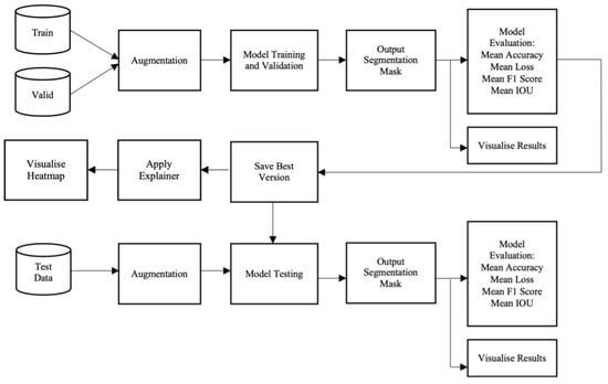
Figure 4.
Data pipeline for the experiments.
The 446 Sentinel-1 and Sentinel-2 images are split into training, validation, and testing sets with sample sizes of 251, 89, and 90, respectively. The data are loaded with a batch size of 16 to accommodate processing limitations, and are shuffled for each epoch, aiding in the reduction of the possibility of overfitting. The Cross Entropy Loss function is employed, which is a measure of the difference between the probability distributions of the true and predicted values, calculated as shown in Equation (5), where is the true value and is the predicted value, with being the target class.
As in most flood image data, there is a significant imbalance of water to background pixels, with water making up the minority class. Weighting is employed within the loss function in order to overcome this, where the water class is given 8 times the importance of the background class.
Adaptive Moment Estimation with Decoupled Weight Decay (AdamW) is utilized; this is an optimization technique based on stochastic gradient descent. It dynamically estimates first-order and second-order moments, offering adaptive adjustments during training. In AdamW the weight decay method is enhanced through decoupling it from the optimization steps [43]. The learning rate is set to 0.0005, scheduled with Cosine Annealing Warm Restarts, where the learning rate is decreased from a high value to a low value, and then restarts from the previously found ‘good’ value [44]. The model is trained and validated over 250 epochs, while being evaluated on the accuracy, loss, F1 score, and Intersection Over Union (IOU) every 10 epochs, which are calculated as follows:
IOU is typically considered to be the most valuable metric for evaluating semantic-segmentation models, as it is able to quantify how effectively the predicted mask overlaps with the ground truth. Therefore, the version of the model with the highest validation IOU is saved for testing.
3. Results
3.1. Comparison of Models
To contextualize the performance of the proposed model outlined in Section 2.2, comparative analysis was conducted against three state-of-the-art models, U-Net++ [38], DeepLabV3+ [45] and Multi-Scale Attention Network (MA-Net) [46], each with a backbone of ResNet50 [47] and MobileNet_V2 [48]. U-Net++ leverages dense skip connections and deep supervision, whereas DeepLabV3+ incorporates atrous convolution and spatial pyramid pooling and MA-Net introduces self-attention mechanisms to adaptively integrate local features with their global dependencies; these consist of a position-wise attention block and a multi-scale fusion attention block, which capture the spatial dependencies between feature maps and the rich multi-scale semantic information of feature maps, respectively. ResNet50 is made up of residual blocks, which each consist of 3 × 3 convolution, batch normalization, and ReLU activation, as well as skip connections; MobileNet_V2 leverages low-dimensional compressed representations as input, then filters through lightweight depthwise separable convolution in order to reduce the memory requirements of training the model.
3.1.1. Quantitative Evaluation
In Table 3, Table 4 and Table 5 the mean accuracy, loss, F1 Score, and IOU are shown for each of the compared models during training, validation, and testing, respectively, with Sentinel-1 images being employed. These results show that the proposed model was able to consistently outperform each of the state-of-the-art models, showcasing its effectiveness in handling Sentinel-1 imagery, and its superior robustness and ability to generalize to unseen data, making it the most suitable for practical flood mapping applications with Sentinel-1 imagery.

Table 3.
Training scores with Sentinel-1 images.

Table 4.
Validation scores with Sentinel-1 images.

Table 5.
Testing scores with Sentinel-1 images.
Table 6, Table 7 and Table 8 show the mean accuracy, loss, F1 Score, and IOU during the training, validation, and testing of the models trained with Sentinel-2 images, where the superiority of the proposed model was further emphasized. Of the state-of-the-art models, U-Net++ with ResNet50 was the best performing with Sentinel-1 images; however, with Sentinel-2 images U-Net++ with MobileNet_V2 exhibits superior performance, suggesting that each state-of-the-art model is better suited to a particular data type. The proposed model, however, outperformed each of the state-of-the-art models across both image types. This demonstrates its ability to adapt to both SAR and optical image sources, further reinforcing its suitability for practical applications, as it will provide consistently high performance regardless of available data.

Table 6.
Training scores with Sentinel-2 images.

Table 7.
Validation scores with Sentinel-2 images.

Table 8.
Testing scores with Sentinel-2 images.
3.1.2. Computational Complexity
Table 9 shows the time taken to train the model for each epoch, and the time taken for inference of an image with both Sentinel-1 and Sentinel-2 in addition to the number of trainable parameters of each model. The state-of-the-art models trained with ResNet50 backbones demonstrated longer training and inference times and a greater number of trainable parameters than their MobileNet_V2 counterparts, with the MA-Net models containing the greatest number of trainable parameters, and the U-Net++ models demonstrating a higher level of computational complexity than the DeepLabV3+ models. The proposed model fell between DeepLabV3+ and U-Net++ with ResNet50 backbones, similar to both MA-Net models in terms of both computation time and number of parameters, providing reduced training and inference time over the MA-Net models and the U-Net++ with ResNet50 backbone. When considered alongside its superior performance, this further emphasizes the suitability of the proposed model for practical use.

Table 9.
Computation time for training and testing with Sentinel-1 images.
3.1.3. Qualitative Evaluation
Visualizations of the flood inundation maps produced by each model for each image type are provided in Figure 5, Figure 6, Figure 7 and Figure 8, with Figure 5 and Figure 7 depicting an example image taken in clear conditions by Sentinel-1 and Sentinel-2, respectively, and Figure 6 and Figure 8 depicting images taken in cloud-covered conditions, providing further insight into how well each model was able to handle different weather conditions present in the imagery. These visualizations revealed that the models exhibiting superior performance against the evaluation metrics tended to produce more refined segmentation masks, resulting in more detailed maps. Conversely, models with weaker performance tended to generate coarser masks, characterized by a higher incidence of false-positive pixel classifications. Notably, the inundation maps produced by the proposed model consistently aligned more closely with the ground truth than did other models.
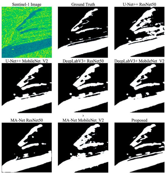
Figure 5.
Sentinel-1 input image, ground truth, and predicted flood inundation maps for an example image in clear conditions.
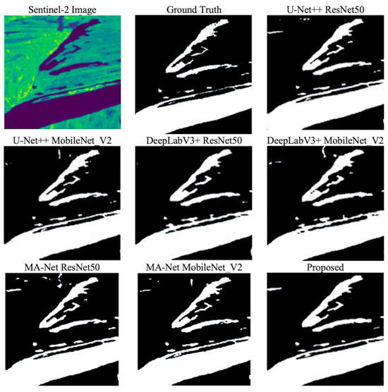
Figure 6.
Sentinel-2 input image, ground truth, and predicted flood inundation maps for an example image in clear conditions.
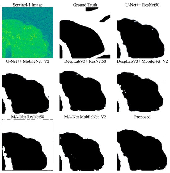
Figure 7.
Sentinel-1 input image, ground truth, and predicted flood inundation maps for an example image in cloud-covered conditions.
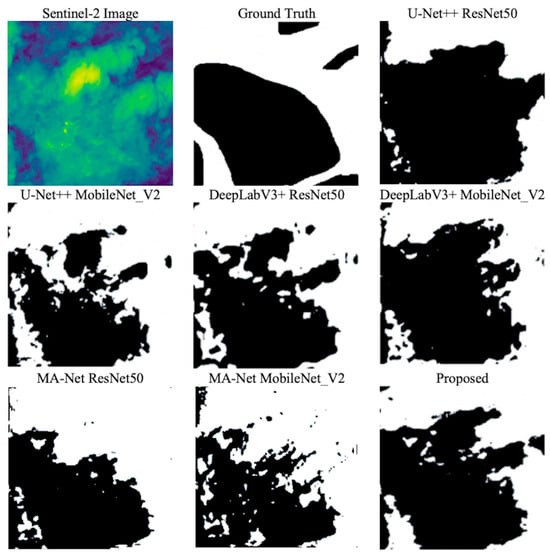
Figure 8.
Sentinel-2 input image, ground truth, and predicted flood inundation maps for an example image in cloud-covered conditions.
In Figure 8, depicting an image sourced from Sentinel-2 under cloudy conditions, the sensor’s visibility was limited, introducing noise into the image. However, even under such challenging circumstances, the proposed model managed to create the most accurate inundation map. This model, in particular, exhibited fewer false-negative areas, which is a crucial factor as it reduces the risk of missing instances of flooding in real-world applications.
To shed light on the decision-making process of the models, the heatmaps generated through gradient-weighted class activation mapping highlighted the areas of the image where the model placed the most importance when making predictions. The color-coded heatmap provided valuable insights into the extent of the model’s attention, where red areas received the highest focus, and dark blue areas received the least. This feature offered more informative data compared to the binary ground truth, as it quantified the presence and significance of the identified features.
The heatmaps for models trained with Sentinel-1 are displayed in Figure 9 and Figure 10, while Figure 11 and Figure 12 illustrate the heatmaps for models trained with Sentinel-2. In general, heatmaps from high-performing models exhibited closer alignment with the ground truth and assigned a higher magnitude of importance to relevant pixels. An exception to this pattern was observed in the case of U-Net++ with the ResNet50 backbone trained with Sentinel-1 images, where the heatmaps revealed the model’s attention to a significant number of irrelevant pixels. Nevertheless, the magnitude of importance attributed to these pixels is minimal, and the areas of higher importance closely corresponded to the ground truth. These heatmaps further emphasize the superior quality of the proposed model, as not only is it able to provide the most accurate flood inundation map, but it is also demonstrably making the most appropriate decisions, applying the highest magnitude of importance to the most relevant pixels of each of the compared models.
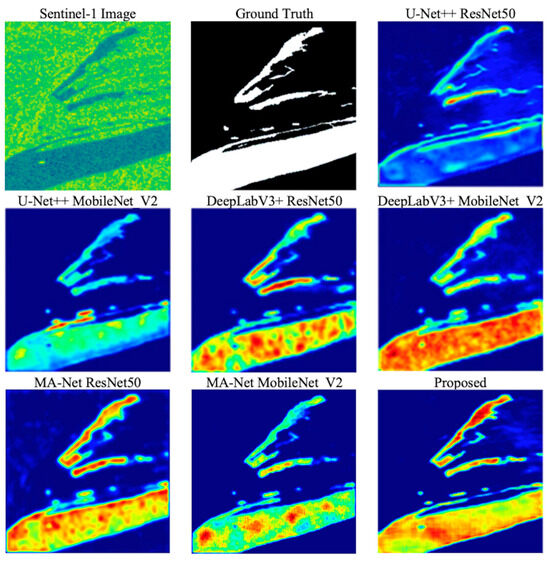
Figure 9.
Sentinel-1 input image, ground truth, and heatmap explanations, with higher temperature (with blue being a low temperature and red a high temperature) indicating greater feature importance, for an example image in clear conditions.
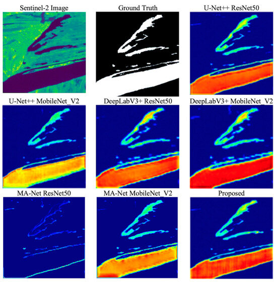
Figure 10.
Sentinel-2 input image, ground truth, and heatmap explanations, with higher temperature (with blue being a low temperature and red a high temperature) indicating greater feature importance, for an example image in clear conditions.
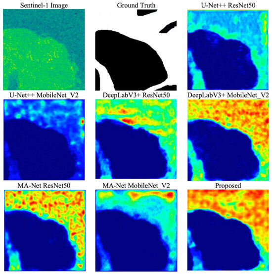
Figure 11.
Sentinel-1 input image, ground truth, and heatmap explanations, with higher temperature (with blue being a low temperature and red a high temperature) indicating greater feature importance, for an example image in cloud-covered conditions.
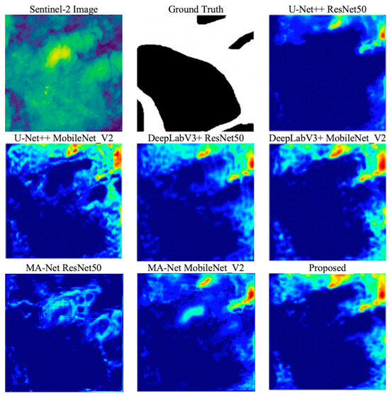
Figure 12.
Sentinel-2 input image, ground truth, and heatmap explanations, with higher temperature (with blue being a low temperature and red a high temperature) indicating greater feature importance, for an example image in cloud-covered conditions.
3.1.4. Ablation Study
To better understand the impact of each module of the proposed model, an ablation study was performed, wherein the model was systematically retrained with one module disabled for each of the modules incorporated in the model. The testing performance of the model with each module removed is shown in Table 10, using the Sentinel-1 images.

Table 10.
Ablation study demonstrating the impact of each module on the performance of the proposed model.
From these results it can be observed that the deep supervision and weighting had the most modest impact on performance, with the model achieving an IOU of 0.5714 and 0.5706, respectively, where the proposed model achieved 0.5862. Conversely, the spatial pyramid pooling and dense skip connections had the most significant influence on the performance of the model, resulting in a reduction of the IOU to 0.5291 and 0.5361, respectively. The atrous convolution had a moderate impact on the performance, where its removal resulted in an IOU of 0.5480.
3.2. Comparison of Sentinel-1 and Sentinel-2 Combinations
3.2.1. Quantitative Evaluation
In Table 11, Table 12 and Table 13 the accuracy, loss, F1 score, and IOU are shown for the proposed model when trained with Sentinel-1, Sentinel-2, and each fusion–configuration of the two satellite image types. It is evident from these tables that in most cases, the fusion of Sentinel-1 and Sentinel-2 bands improved the performance over Sentinel-1 alone but were not able to surpass the performance of Sentinel-2 alone. During training, the only exception to this was where Sentinel-1 was fused with the RGB bands of Sentinel-2, where the performance was weaker than for Sentinel-1 alone. During validation and testing, the fusion of Sentinel-1 with both NDVI and MNDWI also underperformed in comparison to Sentinel-1 alone, which given their superior performance in training suggests potential overfitting and lack of ability to generalize to unseen data. Moreover, the fusion of Sentinel-1 with the RGB, NIR, and SWIR bands of Sentinel-2 provided performance comparable to that of Sentinel-2 alone, and in some cases, such as the training loss and testing IOU was able to outperform Sentinel-2.

Table 11.
Training scores for each combination.

Table 12.
Validation scores for each combination.

Table 13.
Testing scores for each combination.
3.2.2. Qualitative Evaluation
Figure 13 and Figure 14 display the predicted flood inundation maps from each combination of input data in clear and cloud-covered conditions. From Figure 13 it is evident that in clear conditions Sentinel-1 provided a coarser prediction of the flooded area. However, in the Sentinel-2 image, the area in the upper left was falsely identified as a flooded area. In the majority of the combinations, the flooded area prediction was slightly coarser than in the Sentinel-2 image, and the upper left area was falsely identified as flooded. There are, however, some exceptional cases. For instance, from the combinations of VV, VH and RGB; VV, VH, RGB and SWIR; VV, VH and NDVI; and VV, VH and MNDWI, the area in the upper left identified as flooded was significantly reduced. Additionally, from the combinations of VV, VH, RGB and SWIR; and VV, VH, RGB, NIR and SWIR, the predicted maps were at least as finely detailed as the map generated from the Sentinel-2 image.
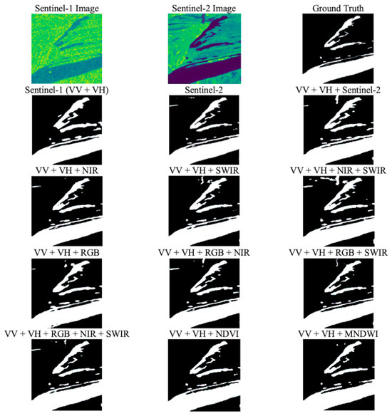
Figure 13.
Sentinel-1 image, Sentinel-2 image, ground truth, and predicted flood inundation maps from each input-data combination for an example image in clear conditions.
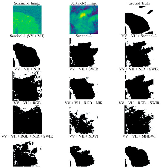
Figure 14.
Sentinel-1 image, Sentinel-2 image, ground truth, and predicted flood inundation maps from each input-data combination for an example image in cloud-covered conditions.
From Figure 14, the weakness of Sentinel-2 in cloud-covered conditions can clearly be observed. Here the Sentinel-1 image significantly outperformed any combination that includes Sentinel-2 information. This issue was much more pronounced for the combinations that included the RGB bands, especially where no supplementary information from NIR and SWIR was provided. The combination of Sentinel-1 with SWIR performed better than any other combination, suggesting that this band is able to penetrate cloud more effectively than the RGB or NIR bands. The combinations with the spectral indices NDVI and MNDWI were also able to produce comparatively accurate maps, suggesting that the extraction of these indices also aids in alleviating the problem of cloud penetration.
Figure 15 and Figure 16 depict the heatmap explanations for the above flood inundation maps, where the magnitude of importance the model placed on each pixel can be observed. From Figure 15, it is evident that in clear conditions, the Sentinel-1 image and the combinations of VV, VH and NIR; VV, VH and SWIR; VV, VH and RGB; VV and VH; and VV, VH and NDVI all resulted in the model having much less confidence in its decision-making, as exemplified by the inconsistency and low magnitude of the heatmaps. Conversely, the models trained with Sentinel-2 or with combinations of Sentinel-1 and Sentinel-2, that is, VV, VH, RGB and SWIR; and VV, VH, RGB, NIR and SWIR, all demonstrated much more appropriate and consistent focus. Notably, in these examples the areas in the upper left which were falsely identified as flooded in the inundation maps had a very low magnitude of importance.
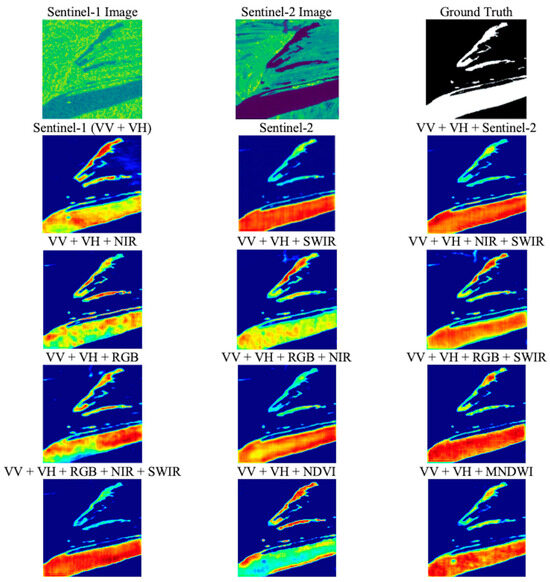
Figure 15.
Sentinel-1 image, Sentinel-2 image, ground truth, and heatmap explanations, with higher temperature (with blue being a low temperature and red a high temperature) indicating greater feature importance, from each input-data combination for an example image in clear conditions.
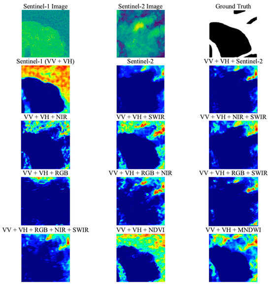
Figure 16.
Sentinel-1 image, Sentinel-2 image, ground truth, and heatmap explanations, with higher temperature (with blue being a low temperature and red a high temperature) indicating greater feature importance, from each input-data combination for an example image in cloud-covered conditions.
The heatmaps shown in Figure 16 show that in cloud-covered conditions, Sentinel-1 was the only image to provide the model with a reasonable level of confidence in its prediction, although the magnitude here was still relatively inconsistent. Although the map generated by the combination of VV, VH and NDVI was less accurate than when the combinations of VV, VH and SWIR; or VV, VH and MNDWI were used, the heatmap showed that this combination was actually placing more consistent and higher magnitude of important on the more relevant areas.
4. Discussion
The proposed model stands out for its capacity to produce flood inundation maps using data from both Sentinel-1 and Sentinel-2 satellites, consistently surpassing the performance of the state-of-the-art segmentation models that were assessed. Notably, the comparative analysis revealed that the U-Net++ with ResNet50 and DeepLabV3+ with MobileNet_V2 models performed better than their counterparts with Sentinel-1 data, whereas U-Net++ with MobileNet_V2 and DeepLabV3+ with ResNet50 performed better with Sentinel-2 data. This presents a challenge when selecting a model for use in a practical setting, as this limits the choice of data. The proposed model, however, consistently demonstrated superior performance across both types of images, making it much more flexible in its practical application. The MA-Net model performed consistently poorly across both data types. It was found in Section 3.1.2 that the computational complexity of this model was significantly higher than the other evaluated models, which given the limited size of the dataset can be attributed to its weak performance. The MA-Net model with the MobileNet_V2 backbone achieved superior performance to its ResNet50 counterpart, and its number of parameters was closer to U-Net++ with ResNet50 and the proposed model, which further emphasizes that this model is too complex to perform well with the small dataset that was employed in this study.
The visualizations of the flood inundation maps further emphasized the quality of the proposed model, as it was consistently able to distinguish the water from the background pixels more accurately than any other assessed model. This is crucial for demonstrating its real-world suitability, as inaccuracies in the flood inundation maps can have significant impact. In the event of false-positive predictions, resources would be needlessly allocated to areas where there is no flood present. False-negative predictions, on the other hand, have more critical implications, as no measures would be put in place to manage the risk of flooding, which could have perilous consequences on human lives and infrastructure.
In examining the impact of the removal of each module of the proposed model, it was found that both deep supervision and weighting exhibited relatively modest effects on performance, suggesting the model’s adaptability to the absence of intermediate supervision signals and the shift from weighted to simple averaging in output fusion, respectively. In contrast, dense skip connections and spatial pyramid pooling, which are crucial for contextual information and multi-scale feature capture, showed more pronounced influences on model performance when removed. The absence of dense skip connections disrupted efficient feature transfer, diminishing contextual awareness and detail capture, resulting in a notable reduction in IOU. Similarly, spatial pyramid pooling’s removal hindered adaptability to diverse object scales, impacting versatility in recognizing spatial dependencies and leading to a decrease in IOU. Atrous convolution demonstrated a moderate impact, indicating its role in balancing spatial context and resolution. These findings underscore the nuanced interplay of architectural elements and their varied contributions to the model’s proficiency in semantic segmentation.
Through the quantitative analysis, it was demonstrated that Sentinel-2 images provided a better-performing model; however, the qualitative analysis revealed more nuance which further emphasizes the importance of the versatility of a flood inundation mapping model. In clear conditions, the flood inundation maps generated from Sentinel-2 images followed expectations of exhibiting greater detail and accuracy than those from Sentinel-1 images; however, in cloud-covered conditions, the Sentinel-2 images had a clear weakness. This contrast means that in a real-world flood inundation mapping system, it may depend on the weather conditions as to which image type is more appropriate, so it is vital that a model is able to adapt well to various types of images.
The heatmap explanations reveal that the proposed model places a more consistent and higher magnitude of importance on the most relevant pixels than any of the other assessed models. This demonstrates that, not only is the model able to make more accurate predictions, but it is also learning more effectively than any of the state-of-the-art models, so can be more easily trusted to make correct decisions in the future.
According to overall model performance, fusion of Sentinel-1 with Sentinel-2 bands and indices is largely unable to match the performance using Sentinel-2 alone, with the exception of the fusion of VV, VH, RGB, NIR and SWIR, which achieves a marginally higher IOU value in testing. The fusion results are, however, generally superior to using Sentinel-1 alone, except where only the RGB bands from Sentinel-2 and the extracted spectral indices NDVI and MNDWI are used. Although this seems to indicate that Sentinel-2 should be the chosen input source for practical applications, the visualizations of the generated flood inundation maps and the heatmap explanations underscore the need for further consideration.
In clear conditions, the accuracy of the flood inundation maps largely follows the expectations given by the overall performance metrics. The magnitude of the heatmaps also exemplifies that the input data that provides better performance also makes the most appropriate decisions, as the magnitude of importance demonstrated in these instances is much more consistent, being higher in the relevant areas and lower in the falsely identified areas. However, in cloud-covered conditions, the results are much more varied. It is evident that Sentinel-1 provides the best map in these cases, with the most appropriate magnitude of importance demonstrated by the heatmaps; however, there are other instances where the accuracy of the inundation maps is still reasonable, but the overall performance of the model is improved over Sentinel-1 alone, in particular the combination of VV, VH and SWIR. In a practical setting, there may be limitations that make it unreasonable to change the input-data type depending on weather conditions, so utilization of this combination may provide a suitable compromise providing better overall performance than Sentinel-1, while still maintaining a reasonable ability to penetrate through cloud.
Previous work involving the fusion of Sentinel-1 and Sentinel-2 images has often focused on using RGB and NIR as the Sentinel-2 bands [49,50,51,52,53] or extracting spectral indices. However, the findings of this study emphasize that the inclusion of SWIR has a more positive impact on the resulting maps than NIR. SWIR, with its longer wavelengths, is better suited to penetrating clouds, which primarily absorb shorter wavelengths. Additionally, it is less affected by atmospheric absorption and exhibits clearer contrast between water bodies and surrounding land, enabling more effective delineation of flooded areas. Deep learning models are highly capable of directly extracting relevant features from raw input data. Therefore, the extraction of spectral indices can introduce redundant features, potentially diminishing the wealth of spectral information available for the model to capture.
5. Conclusions
This study has presented a comprehensive analysis of flood inundation mapping using data from the Sentinel-1 and Sentinel-2 satellites. The proposed model has demonstrated remarkable versatility by consistently outperforming state-of-the-art models when provided with both Sentinel-1 and Sentinel-2 data, affirming its suitability for practical applications.
This study has highlighted the importance of considering various aspects in flood inundation mapping. While quantitative metrics favor Sentinel-2 images, qualitative analysis reveals that the choice of input data is highly dependent on weather conditions. Sentinel-1 excels in cloud-covered conditions. When used in combination with SWIR, it is able to retain reasonable cloud penetration ability, while improving its overall accuracy. On the other hand, Sentinel-2 images outperform Sentinel-1 in clear conditions, providing detailed and accurate flood inundation maps, where the model places a higher magnitude of importance in the most relevant regions of the image. These nuances underscore the significance of a model’s ability to adapt to different data types and environmental conditions.
The extraction of spectral indices, such as NDVI and MNDWI, appears to hinder model performance. Deep learning models excel at feature extraction from raw data, rendering spectral indices redundant and potentially limiting the range of spectral information available for effective modeling.
In practical terms, the results from this study hold significant implications for flood management and disaster response. The ability to accurately predict and map flood inundation in various conditions is essential for timely decision-making and resource allocation. The model proposed in this study is able to generate more accurate flood inundation maps than the state-of-the-art model, and, importantly, its ability to make appropriate decisions has been demonstrated, ensuring that it can be trusted in its application, which is crucial given the direct impact on human lives and infrastructure.
For future work, investigation of the performance of the proposed model when provided with a larger set of input images should be conducted, as larger datasets allow deep learning models to learn complex feature representations more effectively, typically resulting in superior performance, as well as reducing the likelihood of overfitting. Additionally, different types of input data should be further explored. Sentinel-1 and Sentinel-2 are freely available, so represent a clear choice for initial study; however, satellites such as Radarsat-2 provide higher resolution SAR data, which may improve the performance of the model. In optical imaging, hyperspectral images contain a much richer spectral profile, which may aid in improved delineation of flooded areas, so determining the model’s ability to adapt to these images is an important avenue for future research. The incorporation of additional data sources such as Digital Elevation Models (DEM) and Light Detection and Ranging (LiDAR) would also provide more detailed information about the terrain and topography of the area, so will enable the model to generate flood inundation maps with more precision. This detailed information can also enable more detailed and actionable insights through the use of XAI, by providing a deeper understanding of how specific terrain and topographic features influence flood inundation. While the performance of the proposed model is relatively strong, it could be further enhanced through more rigorous hyperparameter tuning as well as postprocessing of the maps generated by the proposed model, with the use of conditional random fields, which can refine the output of a segmentation model. Finally, it was found that the speckle noise of the Sentinel-1 images had a significant negative impact on model performance where these images were employed, so incorporating deep learning-based methods to reduce the noise while preserving object boundaries is another promising area of future research.
Author Contributions
Conceptualization, J.S., H.M. and W.L.W.; methodology, J.S. and W.L.W.; software, J.S.; validation, H.M., M.A.M.A., R.R.O.A.-N. and W.L.W.; resources, J.S.; data curation, J.S.; writing—original draft preparation, J.S. and W.L.W.; writing—review and editing, J.S., H.M., M.A.M.A., R.R.O.A.-N. and W.L.W.; visualization, H.M.; supervision, H.M. and W.L.W.; project administration, W.L.W. All authors have read and agreed to the published version of the manuscript.
Funding
This work is supported as part of the New Generation Flood Resilience (NGFR) project funded by DEFRA in the Flood and Coastal Innovation Programmes.
Data Availability Statement
The data used in this study are available on reasonable request from the corresponding author.
Conflicts of Interest
The authors declare no conflict of interest.
References
- Markus, M.; Angel, J.; Byard, G.; McConkey, S.; Zhang, C.; Cai, X.; Notaro, M.; Ashfaq, M. Communicating the impacts of projected climate change on heavy rainfall using a weighted ensemble approach. J. Hydrol. Eng. 2018, 23, 4018004. [Google Scholar] [CrossRef]
- Mosavi, A.; Ozturk, P.; Chau, K.-W. Flood prediction using machine learning models: Literature review. Water 2018, 10, 1536. [Google Scholar] [CrossRef]
- Leandro, J.; Chen, K.-F.; Wood, R.R.; Ludwig, R. A scalable flood-resilience-index for measuring climate change adaptation: Munich city. Water Res. 2020, 173, 115502. [Google Scholar] [CrossRef] [PubMed]
- Sahana, M.; Patel, P.P. A comparison of frequency ratio and fuzzy logic models for flood susceptibility assessment of the lower Kosi River Basin in India. Environ. Earth Sci. 2019, 78, 289. [Google Scholar] [CrossRef]
- Tavus, B.; Can, R.; Kocaman, S. A Cnn-based flood mapping approach using sentinel-1 data. In ISPRS Annals of the Photogrammetry, Remote Sensing and Spatial Information Sciences; Copernicus GmbH: Göttingen, Germany, 2022; pp. 549–556. [Google Scholar] [CrossRef]
- Li, L.; Chen, Y.; Xu, T.; Meng, L.; Huang, C.; Shi, K. Spatial attraction models coupled with Elman neural networks for enhancing sub-pixel urban inundation mapping. Remote Sens. 2020, 12, 2068. [Google Scholar] [CrossRef]
- Wang, P.; Wang, L.; Leung, H.; Zhang, G. Super-Resolution Mapping Based on Spatial–Spectral Correlation for Spectral Imagery. IEEE Trans. Geosci. Remote Sens. 2021, 59, 2256–2268. [Google Scholar] [CrossRef]
- Costache, R.; Arabameri, A.; Elkhrachy, I.; Ghorbanzadeh, O.; Pham, Q.B. Detection of areas prone to flood risk using state-of-the-art machine learning models. Geomatics Nat. Hazards Risk 2021, 12, 1488–1507. [Google Scholar] [CrossRef]
- Kadiyala, S.P.; Woo, W.L. Flood Prediction and Analysis on the Relevance of Features using Explainable Artificial Intelligence. In Proceedings of the 2021 2nd Artificial Intelligence and Complex Systems Conference, Bangkok, Thailand, 21–22 October 2021; pp. 1–6. [Google Scholar] [CrossRef]
- Pradhan, B.; Lee, S.; Dikshit, A.; Kim, H. Spatial Flood Susceptibility Mapping using and Explainable Artificial Intelligence (XAI) Model. Geosci. Front. 2023, 14, 101625. [Google Scholar] [CrossRef]
- Islam, S.R.; Eberle, W.; Ghafoor, S.K.; Ahmed, M. Explainable Artificial Intelligence Approaches: A Survey. January 2021. Available online: http://arxiv.org/abs/2101.09429 (accessed on 10 October 2023).
- Liang, J.; Liu, D. A local thresholding approach to flood water delineation using Sentinel-1 SAR imagery. ISPRS J. Photogramm. Remote Sens. 2020, 159, 53–62. [Google Scholar] [CrossRef]
- McFeeters, S.K. The use of the Normalized Difference Water Index (NDWI) in the delineation of open water features. Int. J. Remote Sens. 1996, 17, 1425–1432. [Google Scholar] [CrossRef]
- Xu, H. Modification of normalised difference water index (NDWI) to enhance open water features in remotely sensed imagery. Int. J. Remote Sens. 2006, 27, 3025–3033. [Google Scholar] [CrossRef]
- Kriegler, F.J.; Malila, W.A.; Nalepka, R.F.; Richardson, W. Preprocessing Transformations and Their Effects on Multispectral Recognition. In Proceedings of the 6th International Symposium on Remote Sensing and Environment, Ann Arbor, MI, USA, 13 October 1969; pp. 97–131. [Google Scholar]
- Bonafilia, D.; Tellman, B.; Anderson, T.; Issenberg, E. Sen1Floods11: A georeferenced dataset to train and test deep learning flood algorithms for sentinel-1. In Proceedings of the IEEE/CVF Conference on Computer Vision and Pattern Recognition Workshops, Seattle, WA, USA, 13–19 June 2020; pp. 210–211. [Google Scholar] [CrossRef]
- Konapala, G.; Kumar, S.V.; Ahmad, S.K. Exploring Sentinel-1 and Sentinel-2 diversity for flood inundation mapping using deep learning. ISPRS J. Photogramm. Remote Sens. 2021, 180, 163–173. [Google Scholar] [CrossRef]
- Tanim, A.H.; McRae, C.B.; Tavakol-Davani, H.; Goharian, E. Flood Detection in Urban Areas Using Satellite Imagery and Machine Learning. Water 2022, 14, 1140. [Google Scholar] [CrossRef]
- Chakma, P.; Akter, A. Flood Mapping in the Coastal Region of Bangladesh Using Sentinel-1 SAR Images: A Case Study of Super Cyclone Amphan. J. Civ. Eng. Forum 2021, 7, 267–278. [Google Scholar] [CrossRef]
- Dutsenwai, H.S.; Bin Ahmad, B.; Mijinyawa, A.; Tanko, A.I. 37 Fusion of SAR images for flood extent mapping in northern peninsula Malaysia. Int. J. Adv. Appl. Sci. 2016, 3, 37–48. [Google Scholar] [CrossRef]
- Panahi, M.; Rahmati, O.; Kalantari, Z.; Darabi, H.; Rezaie, F.; Moghaddam, D.D.; Ferreira, C.S.S.; Foody, G.; Aliramaee, R.; Bateni, S.M.; et al. Large-scale dynamic flood monitoring in an arid-zone floodplain using SAR data and hybrid machine-learning models. J. Hydrol. 2022, 611, 128001. [Google Scholar] [CrossRef]
- Sundaram, S.; Yarrakula, K. Multi-Temporal Analysis of Sentinel-1 SAR data for Urban Flood Inundation Mapping-Case study of Chennai Metropolitan City Hyperspectral Remote Sensing View Project Risk Mapping Analysis with Geographic Information Systems for a Transportation Network Supply Chain View Project. 2017. Available online: https://www.researchgate.net/publication/322977903 (accessed on 23 July 2023).
- Gebrehiwot, A.; Hashemi-Beni, L. Automated Indunation Mapping: Comparison of Methods. In Proceedings of the International Geoscience and Remote Sensing Symposium (IGARSS), Waikoloa, HI, USA, 26 September–2 October 2020; pp. 3265–3268. [Google Scholar] [CrossRef]
- Fraccaro, P.; Stoyanov, N.; Gaffoor, Z.; La Rosa, L.E.C.; Singh, J.; Ishikawa, T.; Edwards, B.; Jones, A.; Weldermariam, K. Deploying an Artificial Intelligence Application to Detect Flood from Sentinel 1 Data. 2022. Available online: www.aaai.org (accessed on 14 October 2023).
- Ghosh, B.; Garg, S.; Motagh, M. Automatic flood detection from sentinel-1 data using deep learning architectures. In ISPRS Annals of the Photogrammetry, Remote Sensing and Spatial Information Sciences; Copernicus GmbH: Göttingen, Germany, 2022; pp. 201–208. [Google Scholar] [CrossRef]
- Katiyar, V.; Tamkuan, N.; Nagai, M. Near-real-time flood mapping using off-the-shelf models with SAR imagery and deep learning. Remote Sens. 2021, 13, 2334. [Google Scholar] [CrossRef]
- Bereczky, M.; Wieland, M.; Krullikowski, C.; Martinis, S.; Plank, S. Sentinel-1-Based Water and Flood Mapping: Benchmarking Convolutional Neural Networks Against an Operational Rule-Based Processing Chain. IEEE J. Sel. Top. Appl. Earth Obs. Remote Sens. 2022, 15, 2023–2036. [Google Scholar] [CrossRef]
- Li, Z.; Demir, I. U-net-based semantic classification for flood extent extraction using SAR imagery and GEE platform: A case study for 2019 central US flooding. Sci. Total. Environ. 2023, 869, 161757. [Google Scholar] [CrossRef]
- Sanderson, J.; Tengtrairat, N.; Woo, W.L.; Mao, H.; Al-Nima, R.R. XFIMNet: An Explainable Deep Learning Architecture for Versatile Flood Inundation Mapping with Synthetic Aperture Radar and Multi-Spectral Optical Images. Int. J. Remote Sens. 2023. [Google Scholar]
- Paul, S.; Ganju, S. Flood Segmentation on Sentinel-1 SAR Imagery with Semi-Supervised Learning. July 2021. Available online: http://arxiv.org/abs/2107.08369 (accessed on 14 October 2023).
- Yadav, R.; Nascetti, A.; Ban, Y. Attentive Dual Stream Siamese U-net for Flood Detection on Multi-temporal Sentinel-1 Data. In Proceedings of the IGARSS 2022–2022 IEEE International Geoscience and Remote Sensing Symposium, Kuala Lumpur, Malaysia, 17–22 July 2022. [Google Scholar] [CrossRef]
- Jiang, C.; Zhang, H.; Wang, C.; Ge, J.; Wu, F. Water Surface Mapping from Sentinel-1 Imagery Based on Attention-Unet3+: A Case Study of Poyang Lake Region. Remote Sens. 2022, 14, 4708. [Google Scholar] [CrossRef]
- Wang, J.; Wang, S.; Wang, F.; Zhou, Y.; Wang, Z.; Ji, J.; Xiong, Y.; Zhao, Q. FWENet: A deep convolutional neural network for flood water body extraction based on SAR images. Int. J. Digit. Earth 2022, 15, 345–361. [Google Scholar] [CrossRef]
- Zhao, B.; Sui, H.; Liu, J. Siam-DWENet: Flood inundation detection for SAR imagery using a cross-task transfer Siamese network. Int. J. Appl. Earth Obs. Geoinf. 2023, 116, 103132. [Google Scholar] [CrossRef]
- Akiva, P.; Purri, M.; Dana, K.; Tellman, B.; Anderson, T. H2O-Net: Self-Supervised Flood Segmentation via Adversarial Domain Adaptation and Label Refinement. In Proceedings of the IEEE/CVF Winter Conference on Applications of Computer Vision (WACV), Waikoloa, HI, USA, 5 January 2021. [Google Scholar]
- Sediqi, K.M.; Lee, H.J. A novel upsampling and context convolution for image semantic segmentation. Sensors 2021, 21, 2170. [Google Scholar] [CrossRef] [PubMed]
- Lee, C.-Y.; Xie, S.; Gallagher, P.; Zhang, Z.; Tu, Z. Deeply-Supervised Nets. September 2014. Available online: http://arxiv.org/abs/1409.5185 (accessed on 23 October 2023).
- Zhou, Z.; Siddiquee, M.M.R.; Tajbakhsh, N.; Liang, J. Unet++: A nested u-net architecture for medical image segmentation. In Deep Learning in Medical Image Analysis and Multimodal Learning for Clinical Decision Support; Springer: Berlin/Heidelberg, Germany, 2018; pp. 3–11. [Google Scholar] [CrossRef]
- Chen, L.-C.; Papandreou, G.; Kokkinos, I.; Murphy, K.; Yuille, A.L. Deeplab: Semantic image segmentation with deep convolutional nets, atrous convolution, and fully connected crfs. IEEE Trans. Pattern Anal. Mach. Intell. 2017, 40, 834–848. [Google Scholar] [CrossRef] [PubMed]
- He, K.; Zhang, X.; Ren, S.; Sun, J. Spatial pyramid pooling in deep convolutional networks for visual recognition. IEEE Trans. Pattern Anal. Mach. Intell. 2015, 37, 1904–1916. [Google Scholar] [CrossRef] [PubMed]
- Chen, L.-C.; Papandreou, G.; Schroff, F.; Adam, H. Rethinking atrous convolution for semantic image segmentation. arXiv 2017, arXiv:1706.05587. [Google Scholar] [CrossRef]
- Selvaraju, R.R.; Cogswell, M.; Das, A.; Vedantam, R.; Parikh, D.; Batra, D. Grad-CAM: Visual Explanations from Deep Networks via Gradient-based Localization. Int. J. Comput. Vision 2020, 128, 336–359. [Google Scholar] [CrossRef]
- Loshchilov, I.; Hutter, F. Decoupled Weight Decay Regularization. November 2017. Available online: http://arxiv.org/abs/1711.05101 (accessed on 24 October 2023).
- Loshchilov, I.; Hutter, F. Sgdr: Stochastic gradient descent with warm restarts. arXiv 2016, arXiv:1608.03983. [Google Scholar] [CrossRef]
- Chen, L.-C.; Zhu, Y.; Papandreou, G.; Schroff, F.; Adam, H. Encoder-Decoder with Atrous Separable Convolution for Semantic Image Segmentation. February 2018. Available online: http://arxiv.org/abs/1802.02611 (accessed on 23 October 2023).
- Fan, T.; Wang, G.; Li, Y.; Wang, H. Ma-net: A multi-scale attention network for liver and tumor segmentation. IEEE Access 2020, 8, 179656–179665. [Google Scholar] [CrossRef]
- He, K.; Zhang, X.; Ren, S.; Sun, J. Deep residual learning for image recognition. In Proceedings of the IEEE Computer Society Conference on Computer Vision and Pattern Recognition (CVPR), Las Vegas, NV, USA, 27–30 June 2016; pp. 770–778. [Google Scholar] [CrossRef]
- Sandler, M.; Howard, A.; Zhu, M.; Zhmoginov, A.; Chen, L. Mobilenetv2: Inverted residuals and linear bottlenecks. In Proceedings of the IEEE Conference on Computer Vision and Pattern Recognition, Salt Lake City, UT, USA, 18–23 June 2018; pp. 4510–4520. [Google Scholar] [CrossRef]
- He, X.; Zhang, S.; Xue, B.; Zhao, T.; Wu, T. Cross-modal change detection flood extraction based on convolutional neural network. Int. J. Appl. Earth Obs. Geoinf. 2023, 117, 103197. [Google Scholar] [CrossRef]
- Garg, S.; Feinstein, B.; Timnat, S.; Batchu, V.; Dror, G.; Rosenthal, A.G.; Gulshan, V. Cross Modal Distillation for Flood Extent Mapping. February 2023. Available online: http://arxiv.org/abs/2302.08180 (accessed on 13 October 2023).
- Gašparović, M.; Klobučar, D. Mapping floods in lowland forest using sentinel-1 and sentinel-2 data and an object-based approach. Forests 2021, 12, 553. [Google Scholar] [CrossRef]
- Manocha, A.; Afaq, Y.; Bhatia, M. Mapping of water bodies from sentinel-2 images using deep learning-based feature fusion approach. Neural Comput. Appl. 2023, 35, 9167–9179. [Google Scholar] [CrossRef]
- Hosseiny, B.; Mahdianpari, M.; Brisco, B.; Mohammadimanesh, F.; Salehi, B. WetNet: A Spatialoral Ensemble Deep Learning Model for Wetland Classification Using Sentinel-1 and Sentinel-2. IEEE Trans. Geosci. Remote Sens. 2022, 60, 1–14. [Google Scholar] [CrossRef]
Disclaimer/Publisher’s Note: The statements, opinions and data contained in all publications are solely those of the individual author(s) and contributor(s) and not of MDPI and/or the editor(s). MDPI and/or the editor(s) disclaim responsibility for any injury to people or property resulting from any ideas, methods, instructions or products referred to in the content. |
© 2023 by the authors. Licensee MDPI, Basel, Switzerland. This article is an open access article distributed under the terms and conditions of the Creative Commons Attribution (CC BY) license (https://creativecommons.org/licenses/by/4.0/).